Analysis on Mean Time between Failures Based
on Artificial Neural Network
Heqing Li1,2
1 Center South University, Changsha, 410083, China
2 Changsha University of Science and Technology, 410076, Changsha, China Email: [email protected]
Qing Tan
Center South University, Changsha, 410083, China Email: [email protected]
Abstract—Aimed at the reparable characteristic of the mechanical product, a method of the reliability model recognition of mean time between failures based on the BP neural network was developed, and a method of parameter estimation of reliability model based on adaptive linear network was proposed by means of theory of artificial neural network with MATLAB and reliability engineering theory. By network test and numerical simulation, reliability model recognition system and reliability parameters estimation system are verified. The results obtained from the simulation is better than those from the reliability paper for the common reliability model in engineering reliability and indicate the method is feasible. According to the method, the distribution model and function of reliability for mean time between failures of mechanical product were gained by this means.
Index Terms—mean time between failures, model recognition, parameter estimation, artificial neural network
I. INTRODUCTION
In the study of mechanical product reliability, we mainly hope that life distribution law and reliability parameters of random, such as life, material strength and load of mechanical product, are expected to be obtained. Life distribution is one of the main mathematical methods in describing product reliability. If mastering product life distribution, we should be beneficial to improve product reliability and work out scientifically product maintenance strategy. Mean time between failures (MTBF) of product describes mean value of working time between failures. It is able to evaluate manufacture, application and maintenance quality of the product. Thus it is a very important performance index in analyzing the product reliability [1-2].
At present, mechanical product reliability has been widely studied, and we adopt traditionally the methods of graph or mathematical statistical [3-5]. The first method
is direct and rough, but the second one should estimate parameter first and its results depend on the level of accuracy. Recently, neural network has been widely applied in the study of mechanical product reliability. Some scholars have applied neural network to research on life distribution model and parameter estimation of product. Gao Shang has established recognition model of life distribution type through using life data and neural network of training tutor values [6]. Yan Yushan has analyzed on main fan first failure time based on BP neural network technique [7]. Wu Yueming has obtained from the simulation results that indicate BP network needs smaller space occupation and its generalization ability is better than RBF network when solving life distribution model [8]. Ao Changlin has gained the model parameters and function of reliability for the first failure time of a tractor based on neural network [9]. He Yuyang has got the curve of reliability of brake system in vehicles based on BP neural network [10]. Mao Zhaoyong has presented that the improvement genetic algorithms can solve maximum likelihood estimation parameter estimation through neural network, and the result shows that the optimization method of maximum likelihood estimation parameter estimation is feasible [11]. Above methods only individually analyzed reliability model recognition or reliability parameters estimation through neural network theory.
The neural network solving complex relationship among the factors of reliability assessment in nonlinear, discrete system, such as the mechanical product, has unique advantage. Meantime, this method has better mode organization form and computer working platform, therefore, it has broad application prospects. This paper established mechanical product life distribution model and parameters estimation model through neural network. Through above models, the distribution model and parameters estimation model for mean time between failures of the vibratory roller were gained.
II.RECOGNITION SYSTEM OF RELIABILITY MODEL BASED ON BP NEURAL NETWORK
Reliability model plays a virtual role in analyzing product reliability. According to collection of experimentation or field data, some useful information is obtained by analyzing fault data, thus reliability model can be recognized properly. Recognition system of reliability model usually includes fault data pretreatment, feature extraction and classifier.
Because BP neural network has powerful function of pattern matching and nonlinear mapping, it can construct recognition system of complex reliability model.
A. A model structure of BP neural network
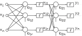
A typical structure of a three layer forward neural network is shown in fig.1. It includes input layer, hidden layer and output layer. In fig.1, circles represent neurons. Connecting line having weight
w
ij between circlesrepresents interaction strength between neurons, where
ij
w
is the connection weight between neuron i in the k-thlayer and neuron j in the (k-1)-th,
b
ki(i=0~n) is the threshold of neurons,x
i(i=0~n) is the input of neurons,j
y
(j=0~m) is the output of neurons and F(·) is a transfer function from the (k-1)-th layer to the k-th layer.Figure 1. Model structure of BP neural network
Structure design of network is related to layers of network, neurons in each layer, initial values and learning rate, etc. After determining structure of BP network, using input and output sample sets train designed network, namely, the weights and thresholds of network is learned and adjusted continually, so that the designed network implements relationship between input and output.
B.Learning algorithm of BP neural network
BP (Back propagation) neural network uses the error of the output layer to estimate the error of the direct precursor layer of the output layer, and then use the error
to estimate the error of the preceding layer again and again. The estimates of error of the other layers again and again. The estimation of error of the other layers can be obtained. In this way, it may form the process that transmits the error of the output layer to the input layer of network along the transmission right about of the input signals. Thereby, the algorithm is called the Back Propagation algorithm. And the non-cycle network that uses the BP algorithm to learn is called BP network. Its course of learning is just the course of training. The training is to adjust the weights among neurons by certain manner when the samples vectors are put into neural network. The specific realizations of BP learning algorithm follow as:
1) Initialize right aggregate wij, get the value of the lesser stochastic nonzero;
2) Give many pairs of input and output samples (Xp, Dp), where p=1, 2, …, p, i is number of training mode pairs; Xp is input vectors, Dp is output expectation vectors.
3)Calculate their actual output Yp=(y1p, y2p, …, ymp), in this course, many times of positive spread calculation is done in terms of the different number of network layer.
4) Evaluate the objective function of the network, and the output error value can generally be denoted as:
∑∑
= =
− =
p
p m
j
jp jp y d E
1 1
2 ) (
2
1 . (1)
5) Judge whether the network satisfies the precision
ε
≤
E . (2)
Where ε is the desired precise, the process of training will continue until the precision is attained.
6) Adjusting the weights through dropping off one by one along the reverse according to grads can be computed by:
ij ij
ij
W E t
W t
W
∂ ∂ − =
+1) () η
( . (3)
TABLE I. PARTS OF LEARNING SAMPLE IN RECOGNITION RELIABILITY DISTRIBUTION
distribution
percentile
0.05 0.15 0.25 0.35 0.45 0.55 0.65 0.75 0.85 0.95
E(0.2) 0.0121 0.0394 0.0697 0.1048 0.1452 0.1915 0.2554 0.3378 0.4622 0.7298
E(0.5) 0.0122 0.0392 0.0698 0.1054 0.1458 0.1948 0.2561 0.3394 0.4644 0.7340
N(1.0,0.2) 0.2130 0.2528 0.2731 0.2887 0.3044 0.3166 0.3320 0.3508 0.3743 0.4080
N(1.0,1.2) -0.2326 -0.0512 0.0401 0.1155 0.1777 0.2346 0.2973 0.3644 0.4661 0.6351
L(1.0,0.3) 0.1733 0.2099 0.2315 0.2562 0.2797 0.3047 0.3287 0.3607 0.4051 0.4831
L(1.0,1.1) 0.0203 0.0365 0.0547 0.0782 0.1024 0.1414 0.1885 0.2622 0.4395 0.7199
W(1.2,1.0) 0.0197 0.0603 0.0932 0.1321 0.1682 0.2160 0.2693 0.3377 0.4359 0.7199
C.Recognition system design of reliability model based on BP neural network.
In designed need recognition types, distribution models are likely to be categorized into four types: exponential, normal, lognormal, and WEIBULL distribution. Method of random simulation by MATLAB produces four sorts of different parameters distributions, which have ten groups of random sequences as the initial sample data individually. Then selection of percentile of statistical features in a probability distribution is regarded as training sample set of recognition system. In order to reduce sample feature absolute value has influence on approximation accuracy, 10 percentiles in each sample is likely to need normalization processing. Parts of learning sample are shown in table 1, E is exponential distribution, N is normal distribution, L is lognormal distribution, and W is two parameters. Density function of WEIBULL distribution is given by:
f
(
t
)
=
(
t
)
−1e
−( )(
t
≥
0
)
t βη β
η
η
β
. (4)Where,
β
is shape parameter, and η is scale parameter.According to recognition types and learning sample, objective response of network is given as follow:
N N N N
⎥
⎥
⎥
⎥
⎥
⎦
⎤
⎢
⎢
⎢
⎢
⎢
⎣
⎡
=
10 10 10 10
1
1
0
0
0
0
0
0
0
10
01
00
0
0
00
10
01
0
0
00
00
10
1
"
"
"
"
"
"
"
"
"
"
"
"
"
"
"
"
y
. (5)After determining the input sample and the output response, unit numbers of the input layer and the output layer are also determined. Experiment indicates that the numbers of layers of BP neural network of recognition reliability model is three. The numbers of neurons of the input layer, hidden layer and output layer are 10, 4, 4 respectively. The transfer function of hidden layer and output layer is a sigmoid function, namely, it is
s e s f
− + =
1 1 )
( . Selection of related parameters: the most
learning times is me=10000, the least expectation error is eg=0.0001, and the learning rate of adaptation of weight is
η=0.01. In process of training network, the change curve of error is shown in fig.2. The sum of squares of error is close to 10-4 through 1351 times training network.
Figure 2. The change curve of the sum of squares of error
Finally, method of random simulation produces respectively 20 groups of exponential, normal, lognormal and WEIBULL distribution as testing sample, trained neural network recognizes these data, its recognition rate is shown in table 2.
III. RELIABILITY PARAMETERS ESTIMATION BASED ON ADAPTIVE LINEAR NEURAL NETWORK
After recognizing reliability model of system, we can design reliability model. Through analyzing related life data of system, distribution law and parameter of random variables can be determined. This paper describes parameter estimation of reliability model of the mechanical product based on adaptive linear neural network.
A. A model structure of the adaptive neural network
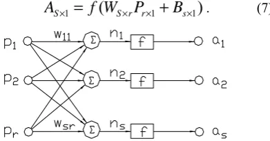
The adaptive linear neural network represents one of the most classical examples of an artificial neural network, being also one of the most simple in terms of the overall design. Model structure of the adaptive linear neural network is shown in fig. 2, which contains r input and s parallel neurons. Each element
P
j (j=1, 2, …, r) in the input vectorP
communicates with each output neuron through weigh matrixW
, each output neuron obtains output vectorA
by a transfer function operation. The input vector of a transfer function is the net input vector of each neuron, whose result is the input vector P multiplied by weight matrixW
. The output vectorA
is given by:
A
S×1=
f
(
W
S×rP
r×1+
B
s×1)
=
W
s×rP
r×1+
B
s×1. (6)Where
f
is a transfer function,s
is node number of the input,r
is node number of the output, andB
is deviation vector.A transfer function in fig. 3 is linear function. The relation between the input vector and the output vector is given by:
A
S×1=
f
(
W
S×rP
r×1+
B
s×1)
. (7)Figure 3. Structure of the adaptive linear neural network
B.Learning algorithm of the adaptive linear neural network
TABLE IV. EXPECTED OUTPUT OF WEIBULL MODEL
number expected
output number
expected
output number
expected
output number
expected
output number
expected output 1 -3.3612 5 -1.3408 9 -0.5873 13 -0.0259 17 0.5354
2 -2.4446 6 -1.1162 10 -0.4380 14 -0.1078 18 0.7048
3 -1.9534 7 -0.9214 11 -0.2965 15 0.2433 19 0.9114
4 -1.6099 8 -0.7469 12 -0.1597 16 0.3845 20 1.2074
TABLE V. MEAN TIME BETWEEN FAILURES OF TWENTY THE VIBRATORY ROLLERS
number MTBF number MTBF number MTBF number MTBF number MTBF
1 310 5 514 9 688 13 951 17 1284
2 319 6 525 10 742 14 1085 18 1395
3 372 7 546 11 742 15 1261 19 1937
4 413 8 599 12 865 16 1282 20 1955
2
(
)
22
1
)
(
2
1
WP
T
A
T
E
=
−
=
−
. (8)Where T represents target vector, namely output expected vector. According to (8), error surface formed by error function of the linear network has properties of parabolic surface. Thus, error function has minimum error value. Based on Widrow-Hoff learning rule, error value is close to minimum by adjusting weights and minimizing the sum of squares of errors. Error value depends on weights and target vector of network. Variation of weight is given by:
i i j
ij
ij
t
a
p
w
E
w
=
−
=
(
−
)
Δ
η
α
α
η
. (9)Where,
Δ
w
ij is variation of weight, andη
is learning rate.(9) also represents by:
Δ
w
ij=
ηδ
ip
j. (10)Where,
δ
i is the error value of the i-th output node.
δ
i=
t
i−
a
i. (11)(10) is named Widrow-Hoff learning rule, also called
δ
learning rule, and least mean square error algorithm. According to Widrow-Hoff learning rule, Variation of weight of network is proportional to output error and input vector. Because it doesn’t calculate differentiation,this algorithm is simple calculation, fast speed and high precision.
C. Numerical simulation
By method of random simulation, WEIBULL distribution data of parameters with β =2.5、η=30 is obtained. These data is shown in table 3. Estimation of reliability given by middle rank is shown in table 4. For the above discussed adaptive linear neural network, program of neural network is written with MATLAB. Neural network have been trained and learned, and its result is given as follow: For WEIBULL distribution of parameters with β =2.5 、η=30 , neural network is trained about 30000 times, and estimation of parameters
β
、η
equals β =2.314、η=30.2459. This result is identical to the result obtained with method of regression analysis, but it is better than the result of β =2.23、07 . 31
=
η obtained with probability paper.
VI. DETERMINING MEAN TIME BETWEEN FAILURE OF THE VIBRATORY ROLLER
A. Statistics of mean time between failures of the vibratory roller
Aimed at collection of using information of the vibratory roller, by analyzing the information, data of mean time between failures of the roller is obtained. It is shown in table 5.
Because reliability of the roller depends on reliability of units and parts, in fault times of view, faults proportion
TABLE III. RANDOM NUMBERS OF WEIBULL DISTRIBUTION
number sample number sample number sample number sample number sample
1 3.7085 5 10.1229 9 14.7378 13 19.0040 17 23.8194
2 5.9020 6 11.5985 10 15.8436 14 19.7509 18 25.9925
3 7.5769 7 12.5008 11 17.2074 15 21.0040 19 30.9143
hydraulic and dynamic system is much higher, accounting for 45.3% and 30.8% total fault individually. Faults of classis system and operation unit account for 15.9% and 8%. From analyzing fault reason, it is mostly caused by quality still and improper maintaining.
B. Recognition mean time between failure model of the vibratory roller based on BP neural network
A great deal of engineering practice and theoretic analysis prove: In general, reliability model of repairable system based on random process obeys exponential distribution and WEIBULL distribution. Data in table 4 are implemented normalization processing, selection of ten arbitrary data is regarded as one group of input vector, other data as another one group of input vector. The above two groups of data are regarded as input vector, which are input to trained BP neural network. According to the output results, we determine much suitable reliability model, and recognition results are given as follow:
y1=0.0651 y2=0.0002 y3=0.0209 y4=0.9242 y5=0.0013 y6=0.0042 y7=0.0674 y8=0.9662 According to the maximal membership principle, compared the output results with objective response, y4=0.9242, and y8=0.9662 are most close to objective response, thus recognition model BP neural network tallies with WEIBULL distribution, the result is in accordance with one obtained by mathematical statistical. So selection of WEIBULL distribution is regarded as reliability model of mean time between failures of the roller.
C. Parameters estimation of mean time between failures of the vibratory roller based on adaptive linear neural network
Based on adaptive linear neural, mean time between failures of the roller obeys parameter estimation of WEIBULL distribution. Density function of mean time between failures, corresponding, failure time distribution function and reliability function are given separately by:
β
η β
η
η
β
) ( 1
)
(
)
(
t
e
t
t
f
=
− − . (12)
F
(
t
)
=
1
−
e
−(ηt)β. (13)
R
(
t
)
=
e
−(ηt)β . (14)Where, β,η(β,η>0) are shape and scale parameter separately.
We select y=ln(−lnR(t)),x=lnt ,thus (14) is
transformed into the following equation.
y=β(x−lnη)=βx−βlnη. (15)
Middle rank is regarded as estimation R(t), namely,
R
(
t
)
1
00..34(
i
1
,
2
,
,
n
)
ni
=
"
−
=
+− . (16)Provided that n equals 20, mean time between failure ti and estimation R(t) are in (16), and (xi, yi) are obtained. The input vector is X=[x1 x2 … xn]/,and objective vector is Y=[y1 y2 … yn ]/. By the adaptive linear neural network, program of neural network is written with MATLAB. Parameters estimation of WEIBULL distribution is obtained as followβ =2.001,η=1001.003. From the above, density
function of mean time between failure of the roller, corresponding failure time distribution function and reliability function are given separately by:
1.001 (1001.003)2.001
003 . 1001 003 .
10012.001 )( ) (
)
(t e t
f = t − . (17)
F
(
t
)
=
1
−
e
−(1001t.003)2.001. (18)
R
(
t
)
=
e
−(1001t.003)2.001. (19)According to the above function, the value of reliability index is calculated in different operation period of the vibratory roller. Aimed at operation state in different period, we shall take some technical and management measures to prevent failure or even accident from occurring.
V. CONCLUSION
On basis of description of the model structure of neural network and the traditional reliability model, the methods of recognition reliability model of the vibratory roller based on BP neural network and parameters estimation of reliability model based on the adaptive linear neural network are proposed. The neural network technique is introduced to analyze reliability model. According to this method, the reliability model and parameters estimation of the model could be quickly obtained if the life data of the known probability distribution was input to the model of the neural network. In practical applications, the method is easy to operate. Meantime, this method offers reference for other product reliability model. By this means, reliability model and parameter estimation of reliability model of mean time between failures of the vibratory roller are obtained.
REFERENCES
[1] Du Feng,Wei Lang, Li Lun. Analysis on failure distribution law and reliability evaluation indices for vehicle products. Transactions of the Chinese of Agricultural Machinery, vol.39, No.1, 2008, pp172-175. [2] Rahman Y.Moghaddam, Michael G.Lipsett. Reliability
assessment and condition monitoring of a shovel test bed. Proceeding of the 3rd world Congress on Engineering Asset Management and Intelligent Maintenance Systems, Beijing, China. 2008, pp1115~1122.
[3] Chi Jie. Study on the failure distribution and reliability variation of the equipment in use. Journal of Changqing Jianzhu University, vol.28, No.5, 2006, pp51-54.
Institute of Architecture and Engineering, vol.25, No.1, 2004, pp71-73.
[5] Jiang Yingshuo, Shao Kai. Reliability analysis of bulldozers. Journal of shenyang Architectural and Civil Engineering Institute, vol.18, No.3, 2002, pp233-236. [6] Shang GAO. Recognition of a life distribution based on a
neural network. International Journal of Plant Engineering and Management, vol.9, No.1, 2004, pp42-45.
[7] Yan Shanyu, Wang Hong de. Analysis on main first failure time based on neural network technique. Journal of China Coal Society, vol.30, No.6, 2005, pp741-745.
[8] Wu Yuming, Wang Yiqun, Li Li. Application study on BP network and generalized RBF network in estimating distribution model of mechanical products. China Mechnical Engnieering, vol.17, No.20, 2006, pp2140-2144. [9] Ao Changlin, Xie Liyang, Dai Youzhong. Parameter
estimation of a tractor reliability model based on Artificial Neural Network. Transactions of the Chinese of Agricultural Machinery, vol.35, No.3, 2004, pp31-33. [10] He Yuyang. Study on reliability of brake system in
vehicles based on artificial neural network. Journal of Hubei Automotive Industries Institute, vol.19, No.3, 2005, pp14-16.
[11] Mao Zhaoyong, Song Baowei, Li Zheng. Optimization method of maximum likelihood estimation parameter based on genetic algorithms. Journal of Mechanical Strength, vol.28, No.1, 2006, pp79-82.
[12] Xie Qingsheng, Ying Jian, Luo Yanke. Artificial Neural Network methods in mechanical engineering. Beijing: China Machine Press, 2003, pp88-98.
[13] Zhou Kaili, Kang Yanghong. Model of the neural network & simulation program design for MATLAB. Beijing: Tsinghua University Press, 2005.pp70-153.
[14] Hagan M T, Howard B Demuth, Mark Beale. Neural network design. New York: PWS Publishing Company, 2002.
[15] FECIT Education Product R&D Center. Neural networks theory and MATLAB7 Application. Beijing: Publishing House of Electronics Industry, 2005.
[16] He Guofang. Collection and analysis of reliable date. Beijing: Nation Defense Industry Press, 1995, pp39-47. [17] Jing Renyan, Zuo Mingjian. Reliability model and
application. Beijing: China Machine Press, 1999, pp46-52. [18] Jiang Hua,Yu Qun. Studying reliability laws of complex
maintainable system based on the stochastic process. Technology Supervision in Petroleum Industry, vol.9, 2000, pp30-34.
Heqing Li Hubei Province, China.
Birthdate: February, 1969, Ph.D. candidate in Center South University. He graduated from Dept. Automobile & Mechanical Engineering, Changsha University of Science and Technology. His research interests include electromechanical integration and reliability system theory.
He is an associate professor of Dept. Automobile & Mechanical Engineering, Changsha University of Science and Technology.
Qing Tan Jiangxi Province, China.
Birthdate: Feb, 1956, Ph.D. in Mechanical and Electrical Engineering. He graduated from Dept. Mechanical and Electrical Engineering, Center South University. His research interests include electromechanical integration and fault diagnosis.