Learning Certifiably Optimal Rule Lists for Categorical Data
Elaine Angelino [email protected]
Department of Electrical Engineering and Computer Sciences University of California, Berkeley, Berkeley, CA 94720
Nicholas Larus-Stone [email protected]
Daniel Alabi [email protected]
Margo Seltzer [email protected]
School of Engineering and Applied Sciences Harvard University, Cambridge, MA 02138
Cynthia Rudin∗ [email protected]
Department of Computer Science and Department of Electrical and Computer Engineering Duke University, Durham, NC 27708
Editor:Maya Gupta
∗To whom correspondence should be addressed.
Abstract
We present the design and implementation of a custom discrete optimization technique for building rule lists over a categorical feature space. Our algorithm produces rule lists with optimal training performance, according to the regularized empirical risk, with a certificate of optimality. By leveraging algorithmic bounds, efficient data structures, and computa-tional reuse, we achieve several orders of magnitude speedup in time and a massive reduc-tion of memory consumpreduc-tion. We demonstrate that our approach produces optimal rule lists on practical problems in seconds. Our results indicate that it is possible to construct optimal sparse rule lists that are approximately as accurate as the COMPAS proprietary risk prediction tool on data from Broward County, Florida, but that are completely inter-pretable. This framework is a novel alternative to CART and other decision tree methods for interpretable modeling.
Keywords: rule lists, decision trees, optimization, interpretable models, criminal justice applications
1. Introduction
As machine learning continues to gain prominence in socially-important decision-making, the interpretability of predictive models remains a crucial problem. Our goal is to build models that are highly predictive, transparent, and easily understood by humans. We use rule lists, also known as decision lists, to achieve this goal. Rule lists are predictive models composed of if-then statements; these models are interpretable because the rules provide a reason for each prediction (Figure 1).
Constructing rule lists, or more generally, decision trees, has been a challenge for more than 30 years; most approaches use greedy splitting techniques (Rivest, 1987; Breiman et al., 1984; Quinlan, 1993). Recent approaches use Bayesian analysis, either to find a locally optimal solution (Chipman et al., 1998) or to explore the search space (Letham et al., 2015;
c
if (age= 18−20) and (sex=male) then predict yes
else if (age= 21−23) and (priors= 2−3) then predict yes
else if (priors >3) then predict yes
else predict no
Figure 1: An example rule list that predicts two-year recidivism for the ProPublica data set, found by CORELS.
Yang et al., 2017). These approaches achieve high accuracy while also managing to run reasonably quickly. However, despite the apparent accuracy of the rule lists generated by these algorithms, there is no way to determine either if the generated rule list is optimal or how close it is to optimal, where optimality is defined with respect to minimization of a regularized loss function.
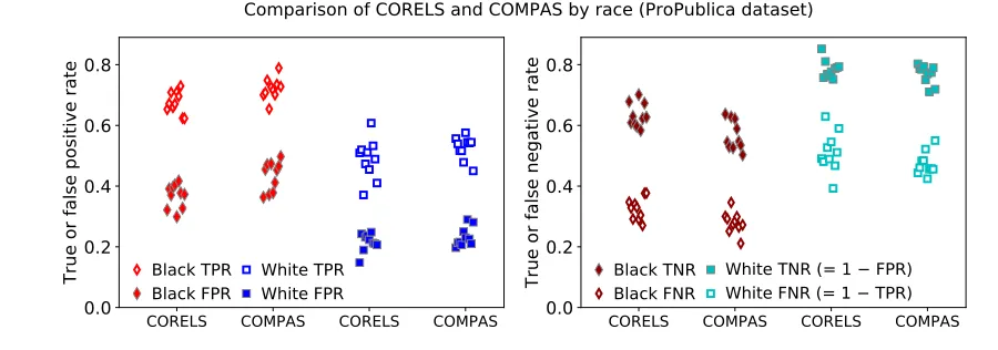
Optimality is important, because there are societal implications for a lack of optimality. Consider the ProPublica article on the Correctional Offender Management Profiling for Al-ternative Sanctions (COMPAS) recidivism prediction tool (Larson et al., 2016). It highlights a case where a black box, proprietary predictive model is being used for recidivism predic-tion. The authors hypothesize that the COMPAS scores are racially biased, but since the model is not transparent, no one (outside of the creators of COMPAS) can determine the reason or extent of the bias (Larson et al., 2016), nor can anyone determine the reason for any particular prediction. By using COMPAS, users implicitly assumed that a transparent model would not be sufficiently accurate for recidivism prediction, i.e., they assumed that a black box model would provide better accuracy. We wondered whether there was indeed no transparent and sufficiently accurate model. Answering this question requires solving a computationally hard problem. Namely, we would like to both find a transparent model that is optimal within a particular pre-determined class of models and produce a certificate of its optimality, with respect to the regularized empirical risk. This would enable one to say, for this problem and model class, with certainty and before resorting to black box methods, whether there exists a transparent model. While there may be differences between train-ing and test performance, findtrain-ing the simplest model with optimal traintrain-ing performance is prescribed by statistical learning theory.
To that end, we consider the class of rule lists assembled from pre-mined frequent item-sets and search for an optimal rule list that minimizes a regularized risk function,R. This is a hard discrete optimization problem. Brute force solutions that minimizeR are compu-tationally prohibitive due to the exponential number of possible rule lists. However, this is a worst case bound that is not realized in practical settings. For realistic cases, it is possible to solve fairly large cases of this problem to optimality, with the careful use of algorithms, data structures, and implementation techniques.
Within its branch-and-bound procedure, CORELS maintains a lower bound on the minimum value of R that each incomplete rule list can achieve. This allows CORELS to prune an incomplete rule list (and every possible extension) if the bound is larger than the error of the best rule list that it has already evaluated. The use of careful bounding techniques leads to massive pruning of the search space of potential rule lists. The algorithm continues to consider incomplete and complete rule lists until it has either examined or eliminated every rule list from consideration. Thus, CORELS terminates with the optimal rule list and a certificate of optimality.
The efficiency of CORELS depends on how much of the search space our bounds allow us to prune; we seek a tight lower bound onR. The bound we maintain throughout execution is a maximum of several bounds that come in three categories. The first category of bounds are those intrinsic to the rules themselves. This category includes bounds stating that each rule must capture sufficient data; if not, the rule list is provably non-optimal. The second type of bound compares a lower bound on the value ofR to that of the current best solution. This allows us to exclude parts of the search space that could never be better than our current solution. Finally, our last type of bound is based on comparing incomplete rule lists that capture the same data and allows us to pursue only the most accurate option. This last class of bounds is especially important—without our use of a novel symmetry-aware map, we are unable to solve most problems of reasonable scale. This symmetry-aware map keeps track of the best accuracy over all observed permutations of a given incomplete rule list.
We keep track of these bounds using a modified prefix tree, a data structure also known as a trie. Each node in the prefix tree represents an individual rule; thus, each path in the tree represents a rule list such that the final node in the path contains metrics about that rule list. This tree structure, together with a search policy and sometimes a queue, enables a variety of strategies, including breadth-first, best-first, and stochastic search. In particular, we can design different best-first strategies by customizing how we order elements in a priority queue. In addition, we are able to limit the number of nodes in the trie and thereby enable tuning of space-time tradeoffs in a robust manner. This trie structure is a useful way of organizing the generation and evaluation of rule lists.
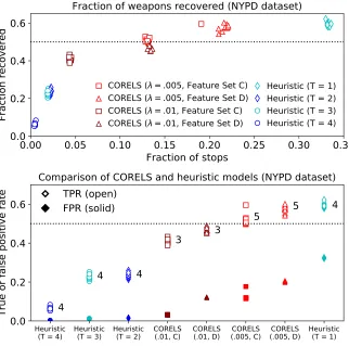
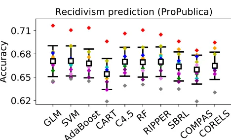
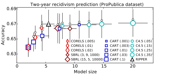
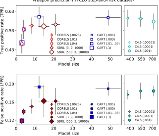
We evaluated CORELS on a number of publicly available data sets. Our metric of success was 10-fold cross-validated prediction accuracy on a subset of the data. These data sets involve hundreds of rules and thousands of observations. CORELS is generally able to find an optimal rule list in a matter of seconds and certify its optimality within about 10 minutes. We show that we are able to achieve better or similar out-of-sample accuracy on these data sets compared to the popular greedy algorithms, CART and C4.5.
Our work overlaps with the thesis of Larus-Stone (2017). We have also written a pre-liminary conference version of this article (Angelino et al., 2017), and a report highlighting systems optimizations of our implementation (Larus-Stone et al., 2018); the latter includes additional empirical measurements not presented here.
Our code is athttps://github.com/nlarusstone/corels, where we provide the C++ implementation we used in our experiments (§6). Kaxiras and Saligrama (2018) have also created an interactive web interface at https://corels.eecs.harvard.edu, where a user can upload data and run CORELS from a browser.
2. Related Work
Since every rule list is a decision tree and every decision tree can be expressed as an equivalent rule list, the problem we are solving is a version of the “optimal decision tree” problem, though regularization changes the nature of the problem (as shown through our bounds). The optimal decision tree problem is computationally hard, though since the late 1990’s, there has been research on building optimal decision trees using optimization tech-niques (Bennett and Blue, 1996; Dobkin et al., 1996; Farhangfar et al., 2008). A particularly interesting paper along these lines is that of Nijssen and Fromont (2010), who created a “bottom-up” way to form optimal decision trees. Their method performs an expensive search step, mining all possible leaves (rather than all possible rules), and uses those leaves to form trees. Their method can lead to memory problems, but it is possible that these memory issues can be mitigated using the theorems in this paper.1 None of these methods used the tight bounds and data structures of CORELS.
Because the optimal decision tree problem is hard, there are a huge number of algo-rithms such as CART (Breiman et al., 1984) and C4.5 (Quinlan, 1993) that do not perform exploration of the search space beyond greedy splitting. Similarly, there are decision list and associative classification methods that construct rule lists iteratively in a greedy way (Rivest, 1987; Liu et al., 1998; Li et al., 2001; Yin and Han, 2003; Sokolova et al., 2003; Marchand and Sokolova, 2005; Vanhoof and Depaire, 2010; Rudin et al., 2013). Some ex-ploration of the search space is done by Bayesian decision tree methods (Dension et al., 1998; Chipman et al., 2002, 2010) and Bayesian rule-based methods (Letham et al., 2015; Yang et al., 2017). The space of trees of a given depth is much larger than the space of rule lists of that same depth, and the trees within the Bayesian tree algorithms are grown in a top-down greedy way. Because of this, authors of Bayesian tree algorithms have noted that their MCMC chains tend to reach only locally optimal solutions. The RIPPER algorithm (Cohen, 1995) is similar to the Bayesian tree methods in that it grows, prunes, and then locally optimizes. The space of rule lists is smaller than that of trees, and has simpler struc-ture. Consequently, Bayesian rule list algorithms tend to be more successful at escaping local minima and can introduce methods of exploring the search space that exploit this structure—these properties motivate our focus on lists. That said, the tightest bounds for the Bayesian lists (namely, those of Yang et al., 2017, upon whose work we build), are not nearly as tight as those of CORELS.
Tight bounds, on the other hand, have been developed for the (immense) literature on building disjunctive normal form (DNF) models; a good example of this is the work of Rijn-beek and Kors (2010). For models of a given size, since the class of DNF’s is a proper subset of decision lists, our framework can be restricted to learn optimal DNF’s. The field of DNF learning includes work from the fields of rule learning/induction (e.g., early algorithms by Michalski, 1969; Clark and Niblett, 1989; Frank and Witten, 1998) and associative classifi-cation (Vanhoof and Depaire, 2010). Most papers in these fields aim to carefully guide the search through the space of models. If we were to place a restriction on our code to learn DNF’s, which would require restricting predictions within the list to the positive class only, we could potentially use methods from rule learning and associative classification to help order CORELS’ queue, which would in turn help us eliminate parts of the search space more quickly.
Some of our bounds, including the minimum support bound (§3.7, Theorem 10), come from Rudin and Ertekin (2016), who provide flexible mixed-integer programming (MIP) formulations using the same objective as we use here; MIP solvers in general cannot compete with the speed of CORELS.
CORELS depends on pre-mined rules, which we obtain here via enumeration. The litera-ture on association rule mining is huge, and any method for rule mining could be reasonably substituted.
CORELS’ main use is for producing interpretable predictive models. There is a grow-ing interest in interpretable (transparent, comprehensible) models because of their societal importance (see R¨uping, 2006; Bratko, 1997; Dawes, 1979; Vellido et al., 2012; Giraud-Carrier, 1998; Holte, 1993; Shmueli, 2010; Huysmans et al., 2011; Freitas, 2014). There are now regulations on algorithmic decision-making in the European Union on the “right to an explanation” (Goodman and Flaxman, 2016) that would legally require interpretability of predictions. There is work in both the DNF literature (R¨uckert and Raedt, 2008) and deci-sion tree literature (Garofalakis et al., 2000) on building interpretable models. Interpretable models must be so sparse that they need to be heavily optimized; heuristics tend to produce either inaccurate or non-sparse models.
Interpretability has many meanings, and it is possible to extend the ideas in this work to other definitions of interpretability; these rule lists may have exotic constraints that help with ease-of-use. For example, Falling Rule Lists (Wang and Rudin, 2015a) are constrained to have decreasing probabilities down the list, which makes it easier to assess whether an observation is in a high risk subgroup. In parallel to this paper, we have been working on an algorithm for Falling Rule Lists (Chen and Rudin, 2018) with bounds similar to those presented here, but even CORELS’ basic support bounds do not hold for the falling case, which is much more complicated. One advantage of the approach taken by Chen and Rudin (2018) is that it can handle class imbalance by weighting the positive and negative classes differently; this extension is possible in CORELS but not addressed here.
if (age= 18−20) and (sex=male)then predict yes
else if(age= 21−23) and (priors= 2−3)then predict yes
else if (priors >3) then predictyes
else predict no
ifp1 then predict q1 else ifp2 then predict q2 else ifp3 then predict q3 else predictq0
Figure 2: The rule list d= (r1, r2, r3, r0). Each rule is of the form rk=pk →qk, for all k= 0, . . . ,3. We can also express this rule list as d= (dp, δp, q0, K), where
dp = (p1, p2, p3), δp = (1,1,1,1), q0= 0, and K= 3. This is the same 3-rule list
as in Figure 1, that predicts two-year recidivism for the ProPublica data set.
help with policy design. CORELS could potentially be adapted to handle these kinds of interesting problems.
3. Learning Optimal Rule Lists
In this section, we present our framework for learning certifiably optimal rule lists. First, we define our setting and useful notation (§3.1) and then the objective function we seek to min-imize (§3.2). Next, we describe the principal structure of our optimization algorithm (§3.3), which depends on a hierarchically structured objective lower bound (§3.4). We then derive a series of additional bounds that we incorporate into our algorithm, because they enable aggressive pruning of our state space.
3.1 Notation
We restrict our setting to binary classification, where rule lists are Boolean functions; this framework is straightforward to generalize to multi-class classification. Let {(xn, yn)}Nn=1
denote training data, where xn∈ {0,1}J are binary features and yn∈ {0,1} are labels. Letx={xn}Nn=1 and y={yn}Nn=1, and letxn,j denote the j-th feature ofxn.
A rule list d= (r1, r2, . . . , rK, r0) of length K≥0 is a (K+ 1)-tuple consisting of K
distinct association rules, rk=pk→qk, for k= 1, . . . , K, followed by a default rule r0.
Figure 2 illustrates a rule list, d= (r1, r2, r3, r0), which for clarity, we sometimes call aK
-rule list. An association -rule r =p→q is an implication corresponding to the conditional statement, “ifp, thenq.” In our setting, an antecedentpis a Boolean assertion that evaluates to either true or false for each datum xn, and a consequent q is a label prediction. For example, (xn,1 = 0)∧(xn,3 = 1)→ (yn= 1) is an association rule. The final default rule r0
in a rule list can be thought of as a special association rule p0→q0 whose antecedent p0
simply asserts true.
Let d= (r1, r2, . . . , rK, r0) be a K-rule list, where rk=pk→qk for each k= 0, . . . , K. We introduce a useful alternate rule list representation:d= (dp, δp, q0, K), where we define
dp= (p1, . . . , pK) to be d’s prefix, δp= (q1, . . . , qK)∈ {0,1}K gives the label predictions associated with dp, and q0∈ {0,1} is the default label prediction. For example, for the
rule list in Figure 1, we would writed= (dp, δp, q0, K), wheredp = (p1, p2, p3),δp= (1,1,1), q0 = 0, and K = 3. Note that ((),(), q0,0) is a well-defined rule list with an empty prefix;
it is completely defined by a single default rule.
For any given space of rule lists, we defineσ(dp) to be the set of all rule lists whose prefixes start with dp:
σ(dp) ={(d0p, δ 0 p, q
0 0, K
0
) :d0p starts with dp}. (1)
Ifdp = (p1, . . . , pK) andd0p = (p1, . . . , pK, pK+1) are two prefixes such thatd0p starts withdp and extends it by a single antecedent, we say that dp is the parent of d0p and that d0p is a child ofdp.
A rule list dclassifies datum xn by providing the label prediction qk of the first rule rk whose antecedent pk is true for xn. We say that an antecedent pk of antecedent list dp captures xn in the context of dp if pk is the first antecedent in dp that evaluates to true forxn. We also say that a prefix captures those data captured by its antecedents; for a rule list d= (dp, δp, q0, K), data not captured by the prefix dp are classified according to the default label prediction q0.
Let β be a set of antecedents. We define cap(xn, β) = 1 if an antecedent in β captures datum xn, and 0 otherwise. For example, let dp and d0p be prefixes such that d0p starts withdp, thend0p captures all the data that dp captures:
{xn: cap(xn, dp)} ⊆ {xn: cap(xn, d0p)}.
Now let dp be an ordered list of antecedents, and letβ be a subset of antecedents indp. Let us define cap(xn, β|dp) = 1 ifβ captures datumxnin the context ofdp,i.e., if the first antecedent indp that evaluates to true forxnis an antecedent in β, and 0 otherwise. Thus, cap(xn, β|dp) = 1 only if cap(xn, β) = 1; cap(xn, β|dp) = 0 either if cap(xn, β) = 0, or if cap(xn, β) = 1 but there is an antecedentα indp, preceding all antecedents in β, such that cap(xn, α) = 1. For example, ifdp = (p1, . . . , pk, . . . , pK) is a prefix, then
cap(xn, pk|dp) = k−1
^
k0=1
¬cap(xn, pk0) !
∧cap(xn, pk)
indicates whether antecedent pk captures datum xn in the context of dp. Now, define supp(β,x) to be the normalized support of β,
supp(β,x) = 1 N
N
X
n=1
cap(xn, β), (2)
and similarly define supp(β,x|dp) to be the normalized support ofβ in the context ofdp,
supp(β,x|dp) = 1 N
N
X
n=1
cap(xn, β|dp), (3)
Next, we address how empirical data constrains rule lists. Given training data (x,y), an antecedent listdp = (p1, . . . , pK) implies a rule list d= (dp, δp, q0, K) with prefixdp, where the label predictions δp = (q1, . . . , qK) and q0 are empirically set to minimize the number
the context ofdp, and the defaultq0 corresponds to the majority label of data not captured
bydp. In the remainder of our presentation, whenever we refer to a rule list with a particular prefix, we implicitly assume these empirically determined label predictions.
Our method is technically an associative classification method since it leverages pre-mined rules.
3.2 Objective Function
We define a simple objective function for a rule list d= (dp, δp, q0, K):
R(d,x,y) =`(d,x,y) +λK. (4)
This objective function is a regularized empirical risk; it consists of a loss `(d,x,y), mea-suring misclassification error, and a regularization term that penalizes longer rule lists. `(d,x,y) is the fraction of training data whose labels are incorrectly predicted by d. In our setting, the regularization parameter λ≥0 is a small constant; e.g., λ= 0.01 can be thought of as adding a penalty equivalent to misclassifying 1% of data when increasing a rule list’s length by one association rule.
3.3 Optimization Framework
Our objective has structure amenable to global optimization via a branch-and-bound frame-work. In particular, we make a series of important observations, each of which translates into a useful bound, and that together interact to eliminate large parts of the search space. We discuss these in depth in what follows:
• Lower bounds on a prefix also hold for every extension of that prefix. (§3.4, Theorem 1)
• If a rule list is not accurate enough with respect to its length, we can prune all extensions of it. (§3.4, Lemma 2)
• We can calculatea priori an upper bound on the maximum length of an optimal rule list. (§3.5, Theorem 6)
• Each rule in an optimal rule list must have support that is sufficiently large. This allows us to construct rule lists from frequent itemsets, while preserving the guarantee that we can find a globally optimal rule list from pre-mined rules. (§3.7, Theorem 10)
• Each rule in an optimal rule list must predict accurately. In particular, the number of observations predicted correctly by each rule in an optimal rule list must be above a threshold. (§3.7, Theorem 11)
• We need only consider the optimal permutation of antecedents in a prefix; we can omit all other permutations. (§3.10, Theorem 15 and Corollary 16)
3.4 Hierarchical Objective Lower Bound
We can decompose the misclassification error in (4) into two contributions corresponding to the prefix and the default rule:
`(d,x,y)≡`p(dp, δp,x,y) +`0(dp, q0,x,y),
wheredp = (p1, . . . , pK) and δp = (q1, . . . , qK);
`p(dp, δp,x,y) = 1 N N X n=1 K X k=1
cap(xn, pk|dp)∧1[qk6=yn] is the fraction of data captured and misclassified by the prefix, and
`0(dp, q0,x,y) =
1 N
N
X
n=1
¬cap(xn, dp)∧1[q0 6=yn]
is the fraction of data not captured by the prefix and misclassified by the default rule. Eliminating the latter error term gives a lower boundb(dp,x,y) on the objective,
b(dp,x,y)≡`p(dp, δp,x,y) +λK ≤R(d,x,y), (5)
where we have suppressed the lower bound’s dependence on label predictions δp because they are fully determined, given (dp,x,y). Furthermore, as we state next in Theorem 1, b(dp,x,y) gives a lower bound on the objective ofany rule list whose prefix starts withdp.
Theorem 1 (Hierarchical objective lower bound) Define b(dp,x,y) as in (5). Also,
define σ(dp) to be the set of all rule lists whose prefixes starts with dp, as in (1). Let d= (dp, δp, q0, K) be a rule list with prefix dp, and let d0 = (d0p, δ0p, q00, K0) ∈ σ(dp) be any rule
list such that its prefixd0p starts with dp and K0 ≥K, then b(dp,x,y)≤ R(d0,x,y).
Proof Letdp = (p1, . . . , pK) andδp = (q1, . . . , qK); letd0p= (p1, . . . , pK, pK+1, . . . , pK0) and δp0 = (q1, . . . , qK, qK+1, . . . , qK0). Notice thatd0p yields the same mistakes asdp, and possibly additional mistakes:
`p(d0p, δ 0
p,x,y) = 1 N N X n=1 K0 X k=1
cap(xn, pk|d0p)∧1[qk6=yn]
= 1 N N X n=1 K X k=1
cap(xn, pk|dp)∧1[qk6=yn] + K0 X
k=K+1
cap(xn, pk|d0p)∧1[qk6=yn]
!
=`p(dp, δp,x,y) + 1 N N X n=1 K0 X
k=K+1
cap(xn, pk|d0p)∧1[qk6=yn]≥`p(dp, δp,x,y), (6)
where in the second equality we have used the fact that cap(xn, pk|d0p) = cap(xn, pk|dp) for 1≤k≤K. It follows that
b(dp,x,y) =`p(dp, δp,x,y) +λK ≤`p(d0p, δ
0
p,x,y) +λK 0
Algorithm 1 Branch-and-bound for learning rule lists.
Input:Objective functionR(d,x,y), objective lower boundb(dp,x,y), set of antecedents S ={sm}Mm=1, training data (x,y) = {(xn, yn)}Nn=1, initial best known rule list d0 with
objective R0 =R(d0,x,y); d0 could be obtained as output from another (approximate)
algorithm, otherwise, (d0, R0) = (null,1) provide reasonable default values
Output: Provably optimal rule listd∗ with minimum objectiveR∗
(dc, Rc)←(d0, R0) . Initialize best rule list and objective
Q← queue( [ ( ) ] ) . Initialize queue with empty prefix
while Qnot empty do .Stop when queue is empty
dp ←Q.pop( ) . Remove prefix dp from the queue
d←(dp, δp, q0, K) .Set label predictions δp and q0 to minimize training error if b(dp,x,y)< Rcthen .Bound: Apply Theorem 1
R ←R(d,x,y) .Compute objective ofdp’s rule listd
if R < Rcthen . Update best rule list and objective (dc, Rc)←(d, R)
end if
for sinS do . Branch: Enqueuedp’s children
if snot in dp then Q.push( (dp, s) ) end if
end for end if end while
(d∗, R∗)←(dc, Rc) . Identify provably optimal solution
To generalize, consider a sequence of prefixes such that each prefix starts with all previ-ous prefixes in the sequence. It follows that the corresponding sequence of objective lower bounds increases monotonically. This is precisely the structure required and exploited by branch-and-bound, illustrated in Algorithm 1.
Specifically, the objective lower bound in Theorem 1 enables us to prune the state space hierarchically. While executing branch-and-bound, we keep track of the current best (smallest) objective Rc, thus it is a dynamic, monotonically decreasing quantity. If we encounter a prefixdp with lower boundb(dp,x,y)≥Rc, then by Theorem 1, we do not need to considerany rule listd0 ∈σ(dp) whose prefixd0p starts withdp. For the objective of such a rule list, the current best objective provides a lower bound,i.e.,R(d0,x,y)≥b(d0p,x,y)≥
b(dp,x,y)≥Rc, and thus d0 cannot be optimal.
Next, we state an immediate consequence of Theorem 1.
Lemma 2 (Objective lower bound with one-step lookahead) Let dp be a K-prefix
Proof By the definition of the lower bound (5), which includes the penalty for longer prefixes,
R(d0p,x, y)≥b(d0p,x,y) =`p(d0p, δ 0
p,x,y) +λK 0
=`p(d0p, δ0p,x,y) +λK+λ(K0−K)
=b(dp,x,y) +λ(K0−K)≥b(dp,x,y) +λ≥Rc. (8)
Therefore, even if we encounter a prefix dp with lower bound b(dp,x,y)≤Rc, as long as b(dp,x,y) +λ≥Rc, then we can prune all prefixes d0p that start with and are longer thandp.
3.5 Upper Bounds on Prefix Length
In this section, we derive several upper bounds on prefix length:
• The simplest upper bound on prefix length is given by the total number of available antecedents. (Proposition 3)
• The current best objective Rc implies an upper bound on prefix length. (Theorem 4)
• For intuition, we state a version of the above bound that is valid at the start of execution. (Corollary 5)
• By considering specific families of prefixes, we can obtain tighter bounds on prefix length. (Theorem 6)
In the next section (§3.6), we use these results to derive corresponding upper bounds on the number of prefix evaluations made by Algorithm 1.
Proposition 3 (Trivial upper bound on prefix length) Consider a state space of all
rule lists formed from a set of M antecedents, and let L(d) be the length of rule list d.
M provides an upper bound on the length of any optimal rule list d∗ ∈argmindR(d,x,y), i.e.,L(d)≤M.
Proof Rule lists consist of distinct rules by definition.
At any point during branch-and-bound execution, the current best objectiveRcimplies an upper bound on the maximum prefix length we might still have to consider.
Theorem 4 (Upper bound on prefix length) Consider a state space of all rule lists
formed from a set of M antecedents. Let L(d) be the length of rule list dand let Rc be the
current best objective. For all optimal rule lists d∗∈argmindR(d,x,y)
L(d∗)≤min
Rc λ
, M
where λ is the regularization parameter. Furthermore, if dc is a rule list with objective R(dc,x,y) =Rc, length K, and zero misclassification error, then for every optimal rule list d∗∈ argmindR(d,x,y), if dc∈argmindR(d,x,y), then L(d∗)≤K, or otherwise if dc∈/ argmindR(d,x,y), then L(d∗)≤K−1.
Proof For an optimal rule list d∗ with objective R∗,
λL(d∗)≤R∗=R(d∗,x,y) =`(d∗,x,y) +λL(d∗)≤Rc.
The maximum possible length ford∗ occurs when `(d∗,x,y) is minimized; combining with Proposition 3 gives bound (9).
For the rest of the proof, let K∗ =L(d∗) be the length of d∗. If the current best rule listdc has zero misclassification error, then
λK∗≤`(d∗,x,y) +λK∗ =R(d∗,x,y)≤Rc=R(dc,x,y) =λK,
and thus K∗ ≤K. If the current best rule list is suboptimal, i.e.,dc∈/ argmindR(d,x,y), then
λK∗≤`(d∗,x,y) +λK∗ =R(d∗,x,y)< Rc=R(dc,x,y) =λK,
in which case K∗< K,i.e.,K∗ ≤K−1, since K is an integer.
The latter part of Theorem 4 tells us that if we only need to identify a single instance of an optimal rule list d∗ ∈argmindR(d,x,y), and we encounter a perfectK-rule list with zero misclassification error, then we can prune all prefixes of lengthK or greater.
Corollary 5 (Simple upper bound on prefix length) Let L(d) be the length of rule list d. For all optimal rule lists d∗ ∈argmindR(d,x,y),
L(d∗)≤min
1 2λ
, M
. (10)
Proof Letd= ((),(), q0,0) be the empty rule list; it has objectiveR(d,x,y) =`(d,x,y)≤
1/2, which gives an upper bound onRc. Combining with (9) and Proposition 3 gives (10).
For any particular prefix dp, we can obtain potentially tighter upper bounds on prefix length for the family of all prefixes that start withdp.
Theorem 6 (Prefix-specific upper bound on prefix length) Letd= (dp, δp, q0, K)be
a rule list, let d0 = (d0p, δ0p, q00, K0)∈σ(dp) be any rule list such that d0p starts with dp, and
let Rc be the current best objective. Ifd0p has lower bound b(d0p,x,y)< Rc, then
K0<min
K+
Rc−b(d p,x,y) λ
, M
Proof First, note that K0 ≥K, sinced0p starts with dp. Now recall from (7) that
b(dp,x,y) =`p(dp, δp,x,y) +λK ≤`p(d0p, δp0,x,y) +λK0 =b(d0p,x,y),
and from (6) that`p(dp, δp,x,y)≤`p(d0p, δp0,x,y). Combining these bounds and rearranging gives
b(d0p,x,y) =`p(d0p, δp0,x,y) +λK+λ(K0−K)
≥`p(dp, δp,x,y) +λK+λ(K0−K) =b(dp,x,y) +λ(K0−K). (12)
Combining (12) withb(d0p,x,y)< Rcand Proposition 3 gives (11).
We can view Theorem 6 as a generalization of our one-step lookahead bound (Lemma 2), as (11) is equivalently a bound on K0−K, an upper bound on the number of remain-ing ‘steps’ correspondremain-ing to an iterative sequence of sremain-ingle-rule extensions of a prefix dp. Notice that when d= ((),(), q0,0) is the empty rule list, this bound replicates (9), since
b(dp,x,y) = 0.
3.6 Upper Bounds on the Number of Prefix Evaluations
In this section, we use our upper bounds on prefix length from§3.5 to derive corresponding upper bounds on the number of prefix evaluations made by Algorithm 1. First, we present Theorem 7, in which we use information about the state of Algorithm 1’s execution to calculate, for any given execution state, upper bounds on the number of additional prefix evaluations that might be required for the execution to complete. The relevant execution state depends on the current best objective Rc and information about prefixes we are planning to evaluate, i.e., prefixes in the queue Q of Algorithm 1. We define the number
of remaining prefix evaluations as the number of prefixes that are currently in or will be
inserted into the queue.
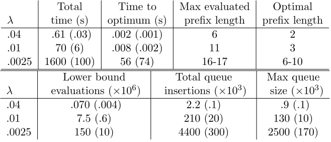
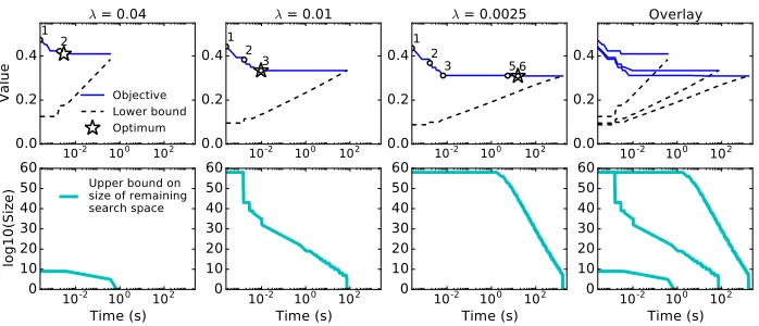
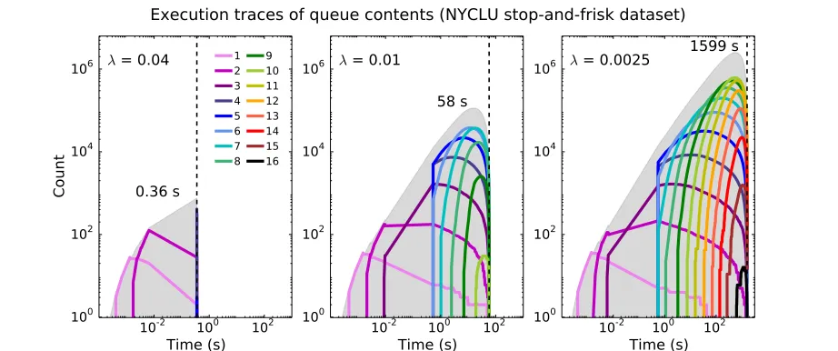
We use Theorem 7 in some of our empirical results (§6, Figure 18) to help illustrate the dramatic impact of certain algorithm optimizations. The execution trace of this upper bound on remaining prefix evaluations complements the execution traces of other quanti-ties, e.g., that of the current best objective Rc. After presenting Theorem 7, we also give two weaker propositions that provide useful intuition. In particular, Proposition 9 is a prac-tical approximation to Theorem 7 that is significantly easier to compute; we use it in our implementation as a metric of execution progress that we display to the user.
Theorem 7 (Fine-grained upper bound on remaining prefix evaluations) Con-sider the state space of all rule lists formed from a set ofM antecedents, and consider Algo-rithm 1 at a particular instant during execution. Let Rc be the current best objective, let Q be the queue, and let L(dp) be the length of prefix dp. Define Γ(Rc, Q) to be the number of
remaining prefix evaluations, then
Γ(Rc, Q)≤ X dp∈Q
f(dp)
X
k=0
(M −L(dp))! (M−L(dp)−k)!
where
f(dp) = min
Rc−b(d p,x,y) λ
, M −L(dp)
.
Proof The number of remaining prefix evaluations is equal to the number of prefixes that are currently in or will be inserted into queueQ. For any such prefix dp, Theorem 6 gives an upper bound on the length of any prefixd0p that starts withdp:
L(d0p)≤min
L(dp) +
Rc−b(dp,x,y) λ
, M
≡U(dp).
This gives an upper bound on the number of remaining prefix evaluations:
Γ(Rc, Q)≤ X dp∈Q
U(dp)−L(dp)
X
k=0
P(M −L(dp), k) =
X
dp∈Q
f(dp)
X
k=0
(M−L(dp))! (M−L(dp)−k)!
,
whereP(m, k) denotes the number of k-permutations ofm.
Proposition 8 is strictly weaker than Theorem 7 and is the starting point for its deriva-tion. It is a na¨ıve upper bound on the total number of prefix evaluations over the course of Algorithm 1’s execution. It only depends on the number of rules and the regularization parameterλ;i.e., unlike Theorem 7, it does not use algorithm execution state to bound the size of the search space.
Proposition 8 (Upper bound on the total number of prefix evaluations) Define Γtot(S) to be the total number of prefixes evaluated by Algorithm 1, given the state space of
all rule lists formed from a set S of M rules. For any setS of M rules,
Γtot(S)≤ K
X
k=0
M! (M−k)!,
where K = min(b1/2λc, M).
Proof By Corollary 5, K ≡min(b1/2λc, M) gives an upper bound on the length of any optimal rule list. Since we can think of our problem as finding the optimal selection and permutation ofk out of M rules, over allk≤K,
Γtot(S)≤1 + K
X
k=1
P(M, k) = K
X
k=0
M! (M−k)!.
queue to constrain the lengths of prefixes in the remaining search space. However, Proposi-tion 9 is weaker than Theorem 7 because it leverages only coarse-grained informaProposi-tion from the queue. Specifically, Theorem 7 is strictly tighter because it additionally incorporates prefix-specific objective lower bound information from prefixes in the queue, which further constrains the lengths of prefixes in the remaining search space.
Proposition 9 (Coarse-grained upper bound on remaining prefix evaluations)
Consider a state space of all rule lists formed from a set of M antecedents, and consider
Algorithm 1 at a particular instant during execution. Let Rc be the current best objective,
let Qbe the queue, and let L(dp)be the length of prefix dp. LetQj be the number of prefixes
of length j in Q,
Qj =
{dp:L(dp) =j, dp ∈Q}
and let J = argmaxdp∈QL(dp) be the length of the longest prefix in Q. Define Γ(Rc, Q) to
be the number of remaining prefix evaluations, then
Γ(Rc, Q)≤ J
X
j=1
Qj K−j
X
k=0
(M−j)! (M−j−k)!
!
,
where K = min(bRc/λc, M).
Proof The number of remaining prefix evaluations is equal to the number of prefixes that are currently in or will be inserted into queueQ. For any such remaining prefixdp, Theorem 4 gives an upper bound on its length; defineKto be this bound:L(dp)≤min(bRc/λc, M)≡K. For any prefix dp in queueQ with lengthL(dp) =j, the maximum number of prefixes that start with dp and remain to be evaluated is:
K−j
X
k=0
P(M −j, k) = K−j
X
k=0
(M−j)! (M −j−k)!,
where P(T, k) denotes the number of k-permutations of T. This gives an upper bound on the number of remaining prefix evaluations:
Γ(Rc, Q)≤ J
X
j=0
Qj K−j
X
k=0
P(M−j, k) !
= J
X
j=0
Qj K−j
X
k=0
(M−j)! (M −j−k)!
!
.
3.7 Lower Bounds on Antecedent Support
Theorem 10 (Lower bound on antecedent support) Let d∗ = (dp, δp, q0, K) be any
optimal rule list with objective R∗, i.e., d∗∈argmindR(d,x,y). For each antecedent pk
in prefix dp= (p1, . . . , pK), the regularization parameter λ provides a lower bound on the
normalized support of pk,
λ≤supp(pk,x|dp). (14)
Proof Let d∗ = (dp, δp, q0, K) be an optimal rule list with prefix dp = (p1, . . . , pK) and labels δp= (q1, . . . , qK). Consider the rule list d= (d0p, δp0, q00, K−1) derived from d∗ by
deleting a rule pi →qi, therefore d0p= (p1, . . . , pi−1, pi+1, . . . , pK) and δ0p= (q1, . . . , qi−1,
qi0+1, . . . , qK0 ), whereq0k need not be the same as qk, fork > iand k= 0.
The largest possible discrepancy betweend∗ and dwould occur if d∗ correctly classified all the data captured bypi, while dmisclassified these data. This gives an upper bound:
R(d,x,y) =`(d,x,y) +λ(K−1)≤`(d∗,x,y) + supp(pi,x|dp) +λ(K−1)
=R(d∗,x,y) + supp(pi,x|dp)−λ
=R∗+ supp(pi,x|dp)−λ (15)
where supp(pi,x|dp) is the normalized support of pi in the context of dp, defined in (3), and the regularization ‘bonus’ comes from the fact thatdis one rule shorter thand∗.
At the same time, we must have R∗≤R(d,x,y) for d∗ to be optimal. Combining this with (15) and rearranging gives (14), therefore the regularization parameter λ provides a lower bound on the support of an antecedent pi in an optimal rule list d∗.
Thus, we can prune a prefix dp if any of its antecedents captures less than a fraction λ of data, even if b(dp,x,y)< R∗. Notice that the bound in Theorem 10 depends on the antecedents, but not the label predictions, and thus does not account for misclassification error. Theorem 11 gives a tighter bound by leveraging this additional information, which specifically tightens the upper bound onR(d,x,y) in (15).
Theorem 11 (Lower bound on accurate antecedent support) Let d∗ be any opti-mal rule list with objective R∗, i.e., d∗ = (dp, δp, q0, K)∈argmindR(d,x,y). Let d∗ have
prefixdp= (p1, . . . , pK) and labels δp = (q1, . . . , qK). For each rulepk→qk in d∗, define ak
to be the fraction of data that are captured by pk and correctly classified:
ak≡ 1 N
N
X
n=1
cap(xn, pk|dp)∧1[qk =yn]. (16)
The regularization parameter λprovides a lower bound on ak:
λ≤ak. (17)
Proof As in Theorem 10, let d= (d0p, δ0p, q00, K−1) be the rule list derived from d∗ by deleting a rule pi →qi. Now, let us define `i to be the portion of R∗ due to this rule’s misclassification error,
`i ≡ 1 N
N
X
n=1
The largest discrepancy betweend∗anddwould occur ifdmisclassified all the data captured by pi. This gives an upper bound on the difference between the misclassification error ofd and d∗:
`(d,x,y)−`(d∗,x,y)≤supp(pi,x|dp)−`i
= 1 N
N
X
n=1
cap(xn, pi|dp)− 1 N
N
X
n=1
cap(xn, pi|dp)∧1[qi 6=yn]
= 1 N
N
X
n=1
cap(xn, pi|dp)∧1[qi =yn] =ai,
where we defined ai in (16). Relating this bound to the objectives ofdand d∗ gives
R(d,x,y) =`(d,x,y) +λ(K−1)≤`(d∗,x,y) +ai+λ(K−1)
=R(d∗,x,y) +ai−λ
=R∗+ai−λ. (18)
Combining (18) with the requirementR∗ ≤R(d,x,y) gives the bound λ≤ai.
Thus, we can prune a prefix if any of its rules correctly classifies less than a fraction λ of data. While the lower bound in Theorem 10 is a sub-condition of the lower bound in Theorem 11, we can still leverage both—since the sub-condition is easier to check, check-ing it first can accelerate pruncheck-ing. In addition to applycheck-ing Theorem 10 in the context of constructing rule lists, we can furthermore apply it in the context of rule mining (§3.1). Specifically, it implies that we should only mine rules with normalized support of at leastλ; we need not mine rules with a smaller fraction of observations.2 In contrast, we can only apply Theorem 11 in the context of constructing rule lists; it depends on the misclassifi-cation error associated with each rule in a rule list, thus it provides a lower bound on the number of observations that each such rule must correctly classify.
3.8 Upper Bound on Antecedent Support
In the previous section (§3.7), we proved lower bounds on antecedent support; in Ap-pendix A, we give an upper bound on antecedent support. Specifically, Theorem 21 shows that an antecedent’s support in a rule list cannot be too similar to the set of data not captured by preceding antecedents in the rule list. In particular, Theorem 21 implies that we should only mine rules with normalized support less than or equal to 1−λ; we need not mine rules with a larger fraction of observations. Note that we do not otherwise use this bound in our implementation, because we did not observe a meaningful benefit in preliminary experiments.
3.9 Antecedent Rejection and its Propagation
In this section, we demonstrate further consequences of our lower (§3.7) and upper bounds (§3.8) on antecedent support, under a unified framework we refer to as antecedent rejec-tion. Letdp = (p1, . . . , pK) be a prefix, and letpk be an antecedent in dp. Definepk to have
insufficient support in dp if it does not obey the bound in (14) of Theorem 10. Define pk to have insufficient accurate support in dp if it does not obey the bound in (17) of Theo-rem 11. Define pk to have excessive support in dp if it does not obey the bound in (37) of Theorem 21 (Appendix A). If pk in the context of dp has insufficient support, insufficient accurate support, or excessive support, let us say that prefixdprejects antecedentpK. Next, in Theorem 12, we describe large classes of related rule lists whose prefixes all reject the same antecedent.
Theorem 12 (Antecedent rejection propagates) For any prefixdp = (p1, . . . , pK), let φ(dp) denote the set of all prefixes d0p such that the set of all antecedents in dp is a subset
of the set of all antecedents in d0p, i.e.,
φ(dp) ={d0p = (p01, . . . , p0K0) s.t. {pk:pk∈dp} ⊆ {p0κ :p0κ ∈d0p}, K0≥K}. (19)
Let d= (dp, δp, q0, K) be a rule list with prefixdp = (p1, . . . , pK−1, pK), such that dp rejects
its last antecedentpK, either becausepK in the context ofdp has insufficient support,
insuf-ficient accurate support, or excessive support. Let dKp −1= (p1, . . . , pK−1) be the first K−1
antecedents of dp. Let D= (Dp,∆p, Q0, κ) be any rule list with prefix Dp = (P1, . . . , PK0−1, PK0, . . . , Pκ) such that Dp starts with DK
0−1
p = (P1, . . . , PK0−1)∈ φ(dKp −1) and antecedent PK0 =pK. It follows that prefix Dp rejects PK0 for the same reason that dp rejects pK, and
furthermore, D cannot be optimal, i.e., D /∈argmind†R(d†,x,y).
Proof Combine Proposition 13, Proposition 14, and Proposition 22. The first two are found below, and the last in Appendix A.
Theorem 12 implies potentially significant computational savings. We know from Theo-rems 10, 11, and 21 that during branch-and-bound execution, if we ever encounter a prefix dp= (p1, . . . , pK−1, pK) that rejects its last antecedent pK, then we can prune dp. By The-orem 12, we can also pruneany prefixd0p whose antecedents contains the set of antecedents in dp, in almost any order, with the constraint that all antecedents in {p1, . . . , pK−1}
pre-cedepK. These latter antecedents are also rejected directly by the bounds in Theorems 10, 11, and 21; this is how our implementation works in practice. In a preliminary implemen-tation (not shown), we maintained additional data structures to support the direct use of Theorem 12. We leave the design of efficient data structures for this task as future work.
Proposition 13 (Insufficient antecedent support propagates) First define φ(dp) as
in (19), and let dp = (p1, . . . , pK−1, pK) be a prefix, such that its last antecedent pK has
insufficient support, i.e., the opposite of the bound in (14):supp(pK,x|dp)< λ. LetdKp −1= (p1, . . . , pK−1), and letD= (Dp,∆p, Q0, κ) be any rule list with prefixDp = (P1, . . . , PK0−1, PK0, . . . , Pκ), such that Dp starts with DK
0−1
p = (P1, . . . , PK0−1)∈φ(dpK−1) and PK0 =pK.
It follows that PK0 has insufficient support in prefix Dp, and furthermore, D cannot be
Proof The support ofpK indpdepends only on the set of antecedents indKp = (p1, . . . , pK):
supp(pK,x|dp) = 1 N
N
X
n=1
cap(xn, pK|dp) = 1 N
N
X
n=1
¬cap(xn, dKp−1)
∧cap(xn, pK)
= 1 N
N
X
n=1 K−1
^
k=1
¬cap(xn, pk)
!
∧cap(xn, pK)< λ,
and the support ofPK0 inDpdepends only on the set of antecedents inDK 0
p = (P1, . . . , PK0):
supp(PK0,x|Dp) = 1 N
N
X
n=1
cap(xn, PK0|Dp) = 1 N
N
X
n=1 K0−1
^
k=1
¬cap(xn, Pk)
!
∧cap(xn, PK0)
≤ 1
N N
X
n=1 K−1
^
k=1
¬cap(xn, pk)
!
∧cap(xn, PK0)
= 1 N
N
X
n=1 K−1
^
k=1
¬cap(xn, pk)
!
∧cap(xn, pK)
= supp(pK,x|dp)< λ. (20)
The first inequality reflects the condition that DK0−1
p ∈φ(dKp −1), which implies that the set of antecedents in DK0−1
p contains the set of antecedents indKp−1, and the next equality reflects the fact that PK0 =pK. Thus, P0
K has insufficient support in prefix Dp, therefore by Theorem 10,D cannot be optimal,i.e.,D /∈argmindR(d,x,y).
Proposition 14 (Insufficient accurate antecedent support propagates) Let φ(dp)
denote the set of all prefixes d0p such that the set of all antecedents in dp is a subset of
the set of all antecedents in d0p, as in (19). Let d= (dp, δp, q0, K) be a rule list with prefix
dp= (p1, . . . , pK) and labels δp = (q1, . . . , qK), such that the last antecedent pK has
insuffi-cient accurate support, i.e., the opposite of the bound in (17):
1 N
N
X
n=1
cap(xn, pK|dp)∧1[qK =yn]< λ.
Let dKp−1 = (p1, . . . , pK−1) and let D= (Dp,∆p, Q0, κ) be any rule list with prefix Dp= (P1, . . . , Pκ)and labels∆p = (Q1, . . . , Qκ), such thatDp starts withDK
0−1
p = (P1, . . . , PK0−1)
∈φ(dKp −1)andPK0 =pK. It follows that PK0 has insufficient accurate support in prefixDp,
Proof The accurate support of PK0 inDp is insufficient:
1 N
N
X
n=1
cap(xn, PK0|Dp)∧1[QK0 =yn]
= 1 N
N
X
n=1 K0−1
^
k=1
¬cap(xn, Pk)
!
∧cap(xn, PK0)∧1[QK0 =yn]
≤ 1
N N
X
n=1 K−1
^
k=1
¬cap(xn, pk)
!
∧cap(xn, PK0)∧1[QK0 =yn]
= 1 N
N
X
n=1 K−1
^
k=1
¬cap(xn, pk)
!
∧cap(xn, pK)∧1[QK0 =yn]
= 1 N
N
X
n=1
cap(xn, pK|dp)∧1[QK0 =yn]
≤ 1
N N
X
n=1
cap(xn, pK|dp)∧1[qK =yn]< λ.
The first inequality reflects the condition thatDKp 0−1 ∈φ(dKp−1), the next equality reflects the fact that PK0 =pK. For the following equality, notice that QK0 is the majority class label of data captured by PK0 in Dp, and qK is the majority class label of data captured byPK indp, and recall from (20) that supp(PK0,x|Dp)≤supp(pK,x|dp). By Theorem 11, D /∈argmind†R(d†,x,y).
Propositions 13 and 14, combined with Proposition 22 (Appendix A), constitute the proof of Theorem 12.
3.10 Equivalent Support Bound
If two prefixes capture the same data, and one is more accurate than the other, then there is no benefit to considering prefixes that start with the less accurate one. Let dp be a prefix, and consider the best possible rule list whose prefix starts with dp. If we take its antecedents indp and replace them with another prefix with the same support (that could include different antecedents), then its objective can only become worse or remain the same. Formally, letDp be a prefix, and letξ(Dp) be the set of all prefixes that capture exactly the same data as Dp. Now, let d be a rule list with prefix dp in ξ(Dp), such that d has the minimum objective over all rule lists with prefixes in ξ(Dp). Finally, let d0 be a rule list whose prefix d0p starts with dp, such that d0 has the minimum objective over all rule lists whose prefixes start withdp. Theorem 15 below implies thatd0 also has the minimum objective over all rule lists whose prefixes start withany prefix inξ(Dp).
Theorem 15 (Equivalent support bound) Define σ(dp) to be the set of all rule lists
whose prefixes start with dp, as in (1). Let d= (dp, δp, q0, K) be a rule list with prefix
such that dp and Dp capture the same data, i.e.,
{xn: cap(xn, dp)}={xn: cap(xn, Dp)}.
If the objective lower bounds ofdand D obeyb(dp,x,y)≤b(Dp,x,y), then the objective of
the optimal rule list in σ(dp) gives a lower bound on the objective of the optimal rule list
in σ(Dp):
min d0∈σ(d
p)
R(d0,x,y)≤ min D0∈σ(D
p)
R(D0,x,y). (21)
Proof See Appendix B for the proof of Theorem 15.
Thus, if prefixesdp andDpcapture the same data, and their objective lower bounds obey b(dp,x,y)≤b(Dp,x,y), Theorem 15 implies that we can pruneDp. Next, in Sections 3.11 and 3.12, we highlight and analyze the special case of prefixes that capture the same data because they contain the same antecedents.
3.11 Permutation Bound
If two prefixes are composed of the same antecedents,i.e., they contain the same antecedents up to a permutation, then they capture the same data, and thus Theorem 15 applies. Therefore, if one is more accurate than the other, then there is no benefit to considering prefixes that start with the less accurate one. Let dp be a prefix, and consider the best possible rule list whose prefix starts with dp. If we permute its antecedents in dp, then its objective can only become worse or remain the same.
Formally, letP ={pk}Kk=1be a set ofKantecedents, and let Π be the set of allK-prefixes
corresponding to permutations of antecedents in P. Let prefix dp in Π have the minimum prefix misclassification error over all prefixes in Π. Also, let d0 be a rule list whose prefixd0p starts withdp, such thatd0 has the minimum objective over all rule lists whose prefixes start with dp. Corollary 16 below, which can be viewed as special case of Theorem 15, implies that d0 also has the minimum objective over all rule lists whose prefixes start with any prefix in Π.
Corollary 16 (Permutation bound) Let π be any permutation of {1, . . . , K}, and de-fine σ(dp) ={(d0p, δ0p, q00, K0) :d0p starts with dp} to be the set of all rule lists whose prefixes
start with dp. Let d= (dp, δp, q0, K) andD= (Dp,∆p, Q0, K)denote rule lists with prefixes
dp= (p1, . . . , pK) and Dp = (pπ(1), . . . , pπ(K)), respectively, i.e., the antecedents in Dp
cor-respond to a permutation of the antecedents in dp. If the objective lower bounds ofdand D
obey b(dp,x,y)≤b(Dp,x,y), then the objective of the optimal rule list in σ(dp) gives a
lower bound on the objective of the optimal rule list in σ(Dp):
min d0∈σ(d
p)
R(d0,x,y)≤ min D0∈σ(D
p)
R(D0,x,y).
Thus if prefixes dp and Dp have the same antecedents, up to a permutation, and their objective lower bounds obey b(dp,x,y)≤ b(Dp,x,y), Corollary 16 implies that we can prune Dp. We call this symmetry-aware pruning, and we illustrate the subsequent compu-tational savings next in§3.12.
3.12 Upper Bound on Prefix Evaluations with Symmetry-aware Pruning
Here, we present an upper bound on the total number of prefix evaluations that accounts for the effect of symmetry-aware pruning (§3.11). Since every subset ofKantecedents generates an equivalence class of K! prefixes equivalent up to permutation, symmetry-aware pruning dramatically reduces the search space.
First, notice that Algorithm 1 describes a breadth-first exploration of the state space of rule lists. Now suppose we integrate symmetry-aware pruning into our execution of branch-and-bound, so that after evaluating prefixes of length K, we only keep a single best prefix from each set of prefixes equivalent up to a permutation.
Theorem 17 (Upper bound on prefix evaluations with symmetry-aware pruning)
Consider a state space of all rule lists formed from a setS of M antecedents, and consider
the branch-and-bound algorithm with symmetry-aware pruning. DefineΓtot(S)to be the total
number of prefixes evaluated. For any set S of M rules,
Γtot(S)≤1 + K
X
k=1
1 (k−1)!·
M! (M−k)!,
where K = min(b1/2λc, M).
Proof By Corollary 5,K ≡min(b1/2λc, M) gives an upper bound on the length of any op-timal rule list. The algorithm begins by evaluating the empty prefix, followed byM prefixes of lengthk= 1, thenP(M,2) prefixes of lengthk= 2, whereP(M,2) is the number of size-2 subsets of{1, . . . , M}. Before proceeding to lengthk= 3, we keep onlyC(M,2) prefixes of lengthk= 2, whereC(M, k) denotes the number ofk-combinations ofM. Now, the number of length k= 3 prefixes we evaluate isC(M,2)(M−2). Propagating this forward gives
Γtot(S)≤1 + K
X
k=1
C(M, k−1)(M −k+ 1) = 1 + K
X
k=1
1 (k−1)! ·
M! (M−k)!.
Pruning based on permutation symmetries thus yields significant computational savings. Let us compare, for example, to the na¨ıve number of prefix evaluations given by the upper bound in Proposition 8. IfM = 100 andK = 5, then the na¨ıve number is about 9.1×10⁹, while the reduced number due to symmetry-aware pruning is about 3.9×10⁸, which is smaller by a factor of about 23. If M = 1000 and K = 10, the number of evaluations falls from about 9.6×1029 to about 2.7×1024, which is smaller by a factor of about 360,000.
our other bounds together conspire to reduce the search space to a size manageable on a single computer. The choice ofM = 1000 andK = 10 in our example above corresponds to the state space size our efforts target. K= 10 rules represents a (heuristic) upper limit on the size of an interpretable rule list, andM = 1000 represents the approximate number of rules with sufficiently high support (Theorem 10) we expect to obtain via rule mining (§3.1).
3.13 Similar Support Bound
We now present a relaxation of Theorem 15, our equivalent support bound. Theorem 18 implies that if we know that no extensions of a prefix dp are better than the current best objective, then we can prune all prefixes with support similar todp’s support. Understanding how to exploit this result in practice represents an exciting direction for future work; our implementation (§5) does not currently leverage the bound in Theorem 18.
Theorem 18 (Similar support bound) Define σ(dp) to be the set of all rule lists whose
prefixes start with dp, as in (1). Let dp = (p1, . . . , pK) and Dp= (P1, . . . , Pκ) be prefixes
that capture nearly the same data. Specifically, defineω to be the normalized support of data captured by dp and not captured by Dp, i.e.,
ω≡ 1
N N
X
n=1
¬cap(xn, Dp)∧cap(xn, dp). (22)
Similarly, define Ω to be the normalized support of data captured by Dp and not captured
by dp, i.e.,
Ω≡ 1
N N
X
n=1
¬cap(xn, dp)∧cap(xn, Dp). (23)
We can bound the difference between the objectives of the optimal rule lists in σ(dp) and
σ(Dp) as follows:
min D†∈σ(D
p)
R(D†,x,y)− min d†∈σ(d
p)
R(d†,x,y)≥b(Dp,x,y)−b(dp,x,y)−ω−Ω, (24)
where b(dp,x,y) and b(Dp,x,y) are the objective lower bounds ofd andD, respectively.
Proof See Appendix C for the proof of Theorem 18.
Theorem 18 implies that if prefixes dp and Dp are similar, and we know the optimal objective of rule lists starting withdp, then
min D0∈σ(D
p)
R(D0,x,y)≥ min d0∈σ(d
p)
R(d0,x,y) +b(Dp,x,y)−b(dp,x,y)−χ
≥Rc+b(Dp,x,y)−b(dp,x,y)−χ,
where Rc is the current best objective, and χ is the normalized support of the set of data captured either exclusively bydp or exclusively by Dp. It follows that
min D0∈σ(D
p)
ifb(Dp,x,y)−b(dp,x,y)≥χ. To conclude, we summarize this result and combine it with our notion of lookahead from Lemma 2. During branch-and-bound execution, if we demon-strate that mind0∈σ(d
p)R(d
0,x,y)≥Rc, then we can prune all prefixes that start with any
prefixD0p in the following set:
(
D0p :b(D0p,x,y) +λ−b(dp,x,y)≥ 1 N
N
X
n=1
cap(xn, dp)⊕cap(xn, D0p)
)
,
where the symbol ⊕denotes the logical operation, exclusive or (XOR).
3.14 Equivalent Points Bound
The bounds in this section quantify the following: If multiple observations that are not captured by a prefix dp have identical features and opposite labels, then no rule list that starts withdpcan correctly classify all these observations. For each set of such observations, the number of mistakes is at least the number of observations with the minority label within the set.
Consider a data set {(xn, yn)}Nn=1 and also a set of antecedents {sm}Mm=1. Define
dis-tinct observations to be equivalent if they are captured by exactly the same antecedents, i.e.,xi 6=xj are equivalent if
1 M
M
X
m=1
1[cap(xi, sm) = cap(xj, sm)] = 1.
Notice that we can partition a data set into sets of equivalent points; let{eu}Uu=1 enumerate
these sets. Leteu be the equivalent points set that contains observationxi. Now defineθ(eu) to be the normalized support of the minority class label with respect to set eu,e.g., let
eu={xn:∀m∈[M],1[cap(xn, sm) = cap(xi, sm)]}, and letqu be the minority class label among points in eu, then
θ(eu) = 1 N
N
X
n=1
1[xn∈eu]1[yn=qu]. (25)
The existence of equivalent points sets with non-singleton support yields a tighter ob-jective lower bound that we can combine with our other bounds; as our experiments demon-strate (§6), the practical consequences can be dramatic. First, for intuition, we present a general bound in Proposition 19; next, we explicitly integrate this bound into our framework in Theorem 20.
Proposition 19 (General equivalent points bound) Letd= (dp, δp, q0, K)be a rule list,
then
R(d,x,y)≥ U
X
u=1
Proof Recall that the objective isR(d,x,y) =`(d,x,y) +λK, where the misclassification error`(d,x,y) is given by
`(d,x,y) =`0(dp, q0,x,y) +`p(dp, δp,x,y) = 1
N N
X
n=1
¬cap(xn, dp)∧1[q0 6=yn] + K
X
k=1
cap(xn, pk|dp)∧1[qk 6=yn]
!
.
Any particular rule list uses a specific rule, and therefore a single class label, to classify all points within a set of equivalent points. Thus, for a set of equivalent points u, the rule listdcorrectly classifies either points that have the majority class label, or points that have the minority class label. It follows that d misclassifies a number of points inu at least as great as the number of points with the minority class label. To translate this into a lower bound on `(d,x,y), we first sum over all sets of equivalent points, and then for each such set, count differences between class labels and the minority class label of the set, instead of counting mistakes:
`(d,x,y)
= 1 N U X u=1 N X n=1
¬cap(xn, dp)∧1[q06=yn] + K
X
k=1
cap(xn, pk|dp)∧1[qk6=yn]
!
1[xn∈eu]
≥ 1 N U X u=1 N X n=1
¬cap(xn, dp)∧1[yn=qu] + K
X
k=1
cap(xn, pk|dp)∧1[yn=qu]
!
1[xn∈eu]. (26)
Next, we factor out the indicator for equivalent point set membership, which yields a term that sums to one, because every datum is either captured or not captured by prefix dp.
`(d,x,y) = 1 N U X u=1 N X n=1
¬cap(xn, dp) + K
X
k=1
cap(xn, pk|dp)
!
∧1[xn∈eu]1[yn=qu]
= 1 N U X u=1 N X n=1
(¬cap(xn, dp) + cap(xn, dp))∧1[xn∈eu]1[yn=qu]
= 1 N U X u=1 N X n=1
1[xn∈eu]1[yn=qu] = U
X
u=1
θ(eu),
where the final equality applies the definition of θ(eu) in (25). Therefore, R(d,x,y) = `(d,x,y) +λK ≥PU
u=1θ(eu) +λK.
Now, recall that to obtain our lower bound b(dp,x,y) in (5), we simply deleted the default rule misclassification error`0(dp, q0,x,y) from the objectiveR(d,x,y). Theorem 20
Theorem 20 (Equivalent points bound) Let d be a rule list with prefix dp and lower
bound b(dp,x,y), then for any rule list d0 ∈σ(d) whose prefix d0p starts with dp,
R(d0,x,y)≥b(dp,x,y) +b0(dp,x,y), (27)
where
b0(dp,x,y) = 1 N
U
X
u=1 N
X
n=1
¬cap(xn, dp)∧1[xn∈eu]1[yn=qu]. (28)
Proof See Appendix D for the proof of Theorem 20.
4. Incremental Computation
For every prefix dp evaluated during Algorithm 1’s execution, we compute the objective lower bound b(dp,x,y) and sometimes the objective R(d,x,y) of the corresponding rule list d. These calculations are the dominant computations with respect to execution time. This motivates our use of a highly optimized library, designed by Yang et al. (2017), for representing rule lists and performing operations encountered in evaluating functions of rule lists. Furthermore, we exploit the hierarchical nature of the objective function and its lower bound to compute these quantities incrementally throughout branch-and-bound execution. In this section, we provide explicit expressions for the incremental computations that are central to our approach. Later, in§5, we describe a cache data structure for supporting our incremental framework in practice.
For completeness, before presenting our incremental expressions, let us begin by writing down the objective lower bound and objective of the empty rule list, d= ((),(), q0,0), the
first rule list evaluated in Algorithm 1. Since its prefix contains zero rules, it has zero prefix misclassification error and also has length zero. Thus, the empty rule list’s objective lower bound is zero,i.e.,b((),x,y) = 0. Since none of the data are captured by the empty prefix, the default rule corresponds to the majority class, and the objective corresponds to the default rule misclassification error, i.e.,R(d,x,y) =`0((), q0,x,y).
Now, we derive our incremental expressions for the objective function and its lower bound. Letd= (dp, δp, q0, K) and d0 = (d0p, δp0, q00, K+ 1) be rule lists such that prefixdp= (p1, . . . , pK) is the parent ofd0p = (p1, . . . , pK, pK+1). Letδp = (q1, . . . , qK) andδ0p= (q1, . . . ,
qK, qK+1) be the corresponding labels. The hierarchical structure of Algorithm 1 enforces
with respect to the objective lower bound of d:
b(d0p,x,y) =`p(d0p, δ0p,x,y) +λ(K+ 1)
= 1 N N X n=1 K+1 X k=1
cap(xn, pk|d0p)∧1[qk6=yn] +λ(K+ 1) (29)
=`p(dp, δp,x,y) +λK+λ+ 1 N
N
X
n=1
cap(xn, pK+1|d0p)∧1[qK+1 6=yn]
=b(dp,x,y) +λ+ 1 N
N
X
n=1
cap(xn, pK+1|d0p)∧1[qK+1 6=yn]
=b(dp,x,y) +λ+ 1 N
N
X
n=1
¬cap(xn, dp)∧cap(xn, pK+1)∧1[qK+1 6=yn]. (30)
Thus, if we store b(dp,x,y), then we can reuse this quantity when computing b(d0p,x,y). Transforming (29) into (30) yields a significantly simpler expression that is a function of the stored quantity b(dp,x,y). For the objective ofd0, first let us write a na¨ıve expression:
R(d0,x,y) =`(d0,x,y) +λ(K+ 1) =`p(d0p, δ 0
p,x,y) +`0(d0p, q 0
0,x,y) +λ(K+ 1)
= 1 N N X n=1 K+1 X k=1
cap(xn, pk|d0p)∧1[qk6=yn] + 1 N
N
X
n=1
¬cap(xn, d0p)∧1[q00 6=yn] +λ(K+ 1). (31)
Instead, we can compute the objective ofd0incrementally with respect to its objective lower bound:
R(d0,x,y) =`p(d0p, δp0,x,y) +`0(d0p, q00,x,y) +λ(K+ 1)
=b(d0p,x,y) +`0(d0p, q 0 0,x,y)
=b(d0p,x,y) + 1 N
N
X
n=1
¬cap(xn, d0p)∧1[q00 6=yn]
=b(d0p,x,y) + 1 N
N
X
n=1
¬cap(xn, dp)∧(¬cap(xn, pK+1))∧1[q00 6=yn]. (32)
The expression in (32) is simpler to compute than that in (31), because the former reuses b(d0p,x,y), which we already computed in (30). Note that instead of computingR(d0,x,y) incrementally from b(d0p,x,y) as in (32), we could have computed it incrementally from R(d,x,y). However, doing so would in practice require that we storeR(d,x,y) in addition to b(dp,x,y), which we already must store to support (30). We prefer the incremental approach suggested by (32) since it avoids this additional storage overhead.
Algorithm 2 Incremental branch-and-bound for learning rule lists, for simplicity, from a cold start. We explicitly show the incremental objective lower bound and objective functions in Algorithms 3 and 4, respectively.
Input:Objective functionR(d,x,y), objective lower boundb(dp,x,y), set of antecedents S ={sm}Mm=1, training data (x,y) ={(xn, yn)}Nn=1, regularization parameterλ
Output: Provably optimal rule listd∗ with minimum objectiveR∗
dc←((),(), q0,0) .Initialize current best rule list with empty rule list
Rc←R(dc,x,y) .Initialize current best objective
Q← queue( [ ( ) ] ) . Initialize queue with empty prefix
C ←cache( [ ( ( ),0 ) ] ).Initialize cache with empty prefix and its objective lower bound
while Qnot empty do .Optimization complete when the queue is empty dp ←Q.pop( ) . Remove a length-K prefixdp from the queue b(dp,x,y)←C.find(dp) . Look up dp’s lower bound in the cache u← ¬cap(x, dp) . Bit vector indicating data not captured bydp
forsinS do . Evaluate all ofdp’s children
if snot indp then
Dp←(dp, s) . Branch: Generate childDp
v←u∧cap(x, s) .Bit vector indicating data captured by sinDp b(Dp,x,y)←b(dp,x,y) +λ+IncrementalLowerBound(v,y, N)
if b(Dp,x,y)< Rcthen .Bound: Apply bound from Theorem 1 R(D,x,y)←b(Dp,x,y) +IncrementalObjective(u,v,y, N)
D←(Dp,∆p, Q0, K+ 1) . ∆p, Q0 are set in the incremental functions if R(D,x,y)< Rc then
(dc, Rc)←(D, R(D,x,y)).Update current best rule list and objective
end if
Q.push(Dp) .Add Dp to the queue
C.insert(Dp, b(Dp,x,y)) .Add Dp and its lower bound to the cache end if
end if end for end while
(d∗, R∗)←(dc, Rc) .Identify provably optimal rule list and objective
Algorithm 3Incremental objective lower bound (30) used in Algorithm 2.
Input: Bit vector v∈ {0,1}N indicating data captured bys, the last antecedent in D p, bit vector of class labels y∈ {0,1}N, number of observations N
Output: Component of D’s misclassification error due to data captured bys
function IncrementalLowerBound(v,y, N)
nv = sum(v) .Number of data captured by s, the last antecedent inDp w←v∧y .Bit vector indicating data captured by swith label 1
nw= sum(w) . Number of data captured byswith label 1
if nw/nv >0.5 then
return (nv−nw)/N .Misclassification error of the rule s→1 else
return nw/N .Misclassification error of the rule s→0 end if
end function
Algorithm 4Incremental objective function (32) used in Algorithm 2.
Input: Bit vector u∈ {0,1}N indicating data not captured by D
p’s parent prefix, bit vector v∈ {0,1}N indicating data not captured by s, the last antecedent in D
p, bit vector of class labelsy∈ {0,1}N, number of observationsN
Output: Component of D’s misclassification error due to its default rule
function IncrementalObjective(u,v,y, N)
f ←u∧ ¬v . Bit vector indicating data not captured byDp
nf = sum(f) . Number of data not captured byDp
g←f∧y . Bit vector indicating data not captured by Dp with label 1
ng= sum(g) . Number of data not captued by Dp with label 1
if ng/nf >0.5 then
return (nf −ng)/N .Misclassification error of the default label prediction 1 else
return ng/N .Misclassification error of the default label prediction 0 end if
end function