Analysis on Multimodal Transportation System

Analysis on Multimodal Transportation System

Mitesh M. Shambharkar Prof. Nikhil H. Pitale

Department of Civil Engineering Department of Civil Engineering

G. H. Raisoni College of Engineering, Nagpur, INDIA G. H. Raisoni College of Engineering, Nagpur, INDIA

Abstract

Human mobility within an urban usually happens over a multimodal transportation network. For that reason, when studying, analysing transportation systems one should not consider each mode of transport separately but one should look to it as multimodal transportation system with relations and dynamics between its components. In order to do any analysis related to transportation a model reflecting the multimodal nature of the system is needed. The objective of the research is to develop a GIS data model for a multimodal transportation system combining different modes in one network that allows different modal combination in route planning.

Keywords: Multimodal transport system, transport system, GIS, Traffic, Traffic signals, Volume flow

________________________________________________________________________________________________________

I. INTRODUCTION

Transport is a critical element of urban system. In present scenario, mega /million plus cities generate more travel demands which is not fully met by either motorized or non-motorized modes. Hence, mass rapid transit system is required as effective means of providing for better, advanced, efficient and quality transit services. However, the efficiency and effective MRTS depends on availability of various modes at city and regional level, location & design of nodes, pedestrian flow at transfer station, etc. Similarly, network structure, line density, stop density, frequency of services, bus routes, etc enhance connectivity and accessibility. Finally, it evolves Multi Modal Transport System (MMTS) which involves the co-coordinated use of different modes and their proper integration to decongest road, reduce journey time, enhance environment and increase running speed. The various characteristics of MMTS are as follows:

- Trips involve more than one mode.

- Use of different modes of transport at different opportunities. - Policy principle not to stick to one single mode.

- Development of seamless web of integrated transport chains, linking road, rail and water ways. - Competition between transporters instead of between transport modes.

- Transfer node and smooth interchange flow.

- Seamless travel an important characteristic of the system.

II. PARAMETERS

Peak Hour Traffic Volume:

The peak hour volume is the volume of traffic that uses the approach, lane, or lane group in question during the hour of the day that observes the highest traffic volumes for that intersection. For example, rush hour might be the peak hour for certain interstate acceleration ramps. The peak hour volume would be the volume of passenger car units that used the ramps during rush hour. Notice the conversion to passenger car units. The peak hour volume is normally given in terms of passenger car units, since changing turning all vehicles into passenger car units makes these volume calculations more representative of what is actually going on.

The peak hour flow rate is also given in passenger car units/hour. Sometimes these two terms are used interchangeably because they are identical numerically.

Peak Hour Factor:

The peak hour factor (PHF) is derived from the peak hour volume. It is simply the ratio of the peak hour volume to four times the peak fifteen-minute volume. For example, during the peak hour, there will probably be a fifteen-minute period in which the traffic volume is denser than during the remainder of the hour. That is the peak fifteen minutes, and the volume of traffic that uses the approach, lane, or lane group during those fifteen minutes is the peak fifteen-minute volume. The peak hour factor is given below.

Peak Hour Factor:

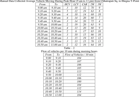
Table – 1

Manual Data Collected Average Vehicle Moving During Peak Hour (9 am to 11 pm) from Chhatrapati Sq. to Hingna T-Point

From To HCV LCV CAR 2W 3W

9.00 am 9.10 am 3 10 12 70 9

9.10 am 9.20 am 5 12 19 63 8

9.20 am 9.30 am 4 10 14 68 10

9.30 am 9.40 am 4 14 20 60 7

9.40 am 9.50 am 3 14 20 72 4

9.50 am 10.00 am 2 19 20 63 9

10.00 am 10.10 am 4 13 20 60 9

10.10 am 10.20 am 2 6 17 65 10

10.20 am 10.30 am 3 10 15 66 10

10.30 am 10.40 am 1 15 19 65 12

10.40 am 10.50 am 3 13 15 70 13

10.50 am 11.00 am 2 12 16 64 10

Table – 2

Flow of vehicles per 10 min during morning hours From To Flow of Vehicles / 10 min

9:00 9:10 104

9:10 9:20 107

9:20 9:30 106

9:30 9:40 105

9:40 9:50 113

9:50 10:00 112

10:00 10:10 106

10:10 10:20 100

10:20 10:30 104

10:30 10:40 112

10:40 10:50 114

10:50 11:00 104

The peak hour volume is just the sum of the volumes of the six 10 minute intervals within the peak hour (640 Vehicles). The peak 10 minute volume is 114 Vehicles in this case. The peak hour factor (PHF) is found by dividing the peak hourvolumebyfourtimesthepeak10minutevolume.

PHF = 640 / (6*114) = 0.936

The Highway Capacity Manual advises that in absence of field measurements reasonable approximations for peak hour factor can be made as follows:

- 0.95 for congested condition - 0.92 for urban areas

- 0.88 for rural areas

The actual (design) flow rate can be calculated by dividing the peak hour volume by the PHF, 640/0.936 = 684vehicles/hr.

Or by multiplying the peak 10 minute volume by six, 6×114=684vehicles/hr. Table – 3

Volumetric Manual Data Collected Average Vehicle Moving During Peak Hour (5 am to 7 pm) from Chhatrapati Sq. to Hingna T-Point

From To HCV LCV CAR 2W 3W

5.00 pm 5.10 pm 3 15 18 72 12

5.10 pm 5.20 pm 2 14 22 65 10

5.20 pm 5.30 pm 3 16 17 68 11

5.30 pm 5.40 pm 3 15 20 62 13

5.40 pm 5.50 pm 2 13 19 76 15

5.50 pm 6.00 pm 2 16 24 66 10

6.00 pm 6.10 pm 3 12 21 64 9

6.10 pm 6.20 pm 1 13 19 68 8

6.20 pm 6.30 pm 2 12 18 71 8

6.30 pm 6.40 pm 1 10 20 69 9

6.40 pm 6.50 pm 2 11 18 74 9

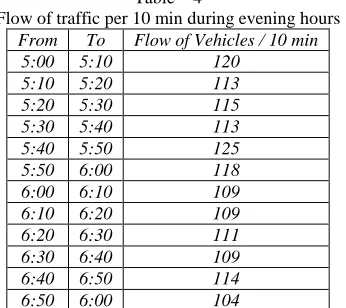
Table – 4

Flow of traffic per 10 min during evening hours From To Flow of Vehicles / 10 min

5:00 5:10 120

5:10 5:20 113

5:20 5:30 115

5:30 5:40 113

5:40 5:50 125

5:50 6:00 118

6:00 6:10 109

6:10 6:20 109

6:20 6:30 111

6:30 6:40 109

6:40 6:50 114

6:50 6:00 104

The peak hour volume is just the sum of the volumes of the six 10 minute intervals within the peak hour(700 Vehicles). The peak 10 minute volume is 114 Vehicles in this case. The peak hour factor(PHF) is found by dividing the peak hourvolumebyfourtimesthepeak10minutevolume.

PHF = 700 / (6*125) = 0.933

The Highway Capacity Manual advises that in absence of field measurements reasonable approximations for peak hour factor can be made as follows:

- 0.95 for congested condition - 0.92 for urban areas

- 0.88 for rural areas

The actual (design) flow rate can be calculated by dividing the peak hour volume by the PHF, 700/0.933 = 750vehicles/hr.,

Or by multiplying the peak 10 minute volume by six, 6×125=750vehicles/hr.

Traffic Composition:

A traffic composition defines the vehicle mix of each input flow to be defined. The relative percentage (proportion) of each vehicle type is to be given.

Table – 5 Traffic Composition

Category Vehicle Dimension (Meter) Projected Area

Car Car, Jeep, Van 3.72 X 1.44 5.39

Bus Bus 10.10 X 2.43 24.74

LCV Mini Bus/ Truck 6.1 X 2.1 12.81

HCV Truck 7.5 X 2.35 17.62

Multi-Axel Truck 2.35 X 12 28.6

Bikes Scooter, Motorbike 1.87 X 0.64 1.2

Autos Auto, Tempo 3.20 X 1.40 4.48

Speed of Vehicles:

As speed defines the distance travelled by user in a given time, and this is a vibrant in every traffic movement. In other words speed of movement is the ratio of distance travelled to time of travel. The actual speed of traffic flow over a given route may fluctuated widely, as because at each time the volume of traffic varies. Accordingly, speeds are generally classified into three main categories

Spot speed this is the instantaneous speed of a vehicle at any specific location.

Running speed this is the average speed maintained over a particular course while the vehicle is in the motion.

Journey speed This is the effective speed of the vehicle on a journey between two points and the distance between two points and the distance between these points divided by the total time taken for the vehicle to complete the journey, it includes all delay. When we measure the traffic parameter over a short distance, we generally measure the spot speed. A spot speed is made by measuring the individual speeds of a sample of the vehicle passing a given spot on a street or highway. Spot speed studies are used to determine the speed distribution of a traffic stream at a specific location. The data gathered in spot speed studies are used to determine vehicle speed percentiles, which are useful in making many speed-related decisions. Spot speed data have a number of safety applications, including the following

4) Geometric design, 5) Research studies.

Calculations:

Step 1 We have to find the mean speed for each vehicle type using the formula:

Where n is the no. of observations and ui is the spot speeds.

Step 2 Find the vehicle values using above formula. Use the table having the areas of various vehicle types given above. Table – 6

Vehicles Mean Speed values using speedometer

Places Car 3 wheeler 2 wheeler LCV HCV

From Chhatrapati sq 16.32 12.67 14.67 10.00 8.40 From Orange City 25.74 18.25 30.27 14.88 10.09 From Pratap Nagar 36.11 30.68 40.75 18.50 14.88 From padole Sq. 26.67 13.98 22.12 12.57 8.38 From Sambhaji Sq. 28.11 18.77 39.52 15.67 15.66 From Trimurty Sq. 37.41 28.77 41.9 19.57 12.66 From Mangal Murty Sq. 38.11 29.52 36.97 15.7 9.55

Hingna T-Point 19.93 16.4 24.97 9.68 6.12

Mean speed ut 28.55 21.13 31.40 14.57 10.72

Signal Timings & Delay:

Traffic flows through signalized intersections are filtered by the signal system (stopping of vehicles during red time) causing vehicular delays. Vehicular delays at signalized intersections will increase the total travel time through an urban road network and ultimately results in the reduction of speed, reliability and cost-effectiveness of the transportation system. The uncontrolled and ill planned growth of urban centers has resulted in a number of problems like traffic congestion, shortage of water and electricity, deteriorating environment and public health. The growing cities have generated the high levels of demand for travel by motor vehicles in the cities. The automobile population in India has increased from a mere 0.3 million in 1951 to more than 45 million in 2001. The registered two wheelers constitute nearly seventy percent of the vehicle population in almost all the cities. More than 90 per cent of the automobiles are located in urban centers. By considering the above factors traffic signals has to be designed in such a way that the flow is organized with less amount of delays.

Table – 7

Variation of control delay for morning peak hour of different intersection (9.00am-11.00am)

Sr. No. Intersections Delay By HCM 2000 (Sec/Veh)

Delay By TSIS

(Sec/Veh) Delay by HCS (Sec/Veh)

1 Chatrapatisq. 41.3 40.1 42.6

2 Khamlasq. 40.6 39.2 41.8

3 Pratapnagarsq. 22.6 17.8 24.5

4 Padolesq. 29.2 20.4 30.4

5 Sambhajisq. 47.6 46.9 49.6

6 Trimurtisq. 39.5 38.8 37.8

7 Mangalmurtisq. 38.4 38.6 39.5

Geometry of Road Design:

Geometric design for transportation facilities includes the design of geometric cross sections, horizontal alignment, vertical alignment, intersections, and various design details.

These basic elements are common to all linear facilities, such as roadways, railways, and airport runways and taxiways. Although the details of design standards vary with the mode and the class of facility, most of the issues involved in geometric design are similar for all modes. In all cases, the goals of geometric design are to maximize the comfort, safety, and economy of facilities, while minimizing their environ- mental impacts.

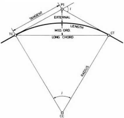
Horizontal alignment

Circular Curves

Fig. 1: Important Components of Simple Circular Curve

Fig. 2:

1) See handout

2) PC, PI, PT, E, M, and  3) L = 2() R ()/360 4) T = R tan (/2)

Fuel Consumption:

The fuel consumption or fuel economy measurement is used to estimate gas mileage and associated fuel cost for a specific vehicle. A mile per gallon (mpg) is a measure of fuel consumption or fuel economy used in the United States. The unit measures how much distance in miles a car can travel on one gallon of fuel. A litre per 100 kilometres is a measure of fuel consumption or fuel economy used in some European countries. The unit measures how many litres (l) of fuel a car consumes to travel one hundred kilometres (100km).

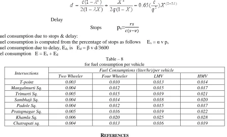
Delay

Stops

p

=

𝑟𝑠 𝑐(𝑠−𝑣) Excess fuel consumption due to stops & delay:

Excess fuel consumption is computed from the percentage of stops as follows Es = α v ps Excess fuel consumption due to delay, Ed, is Ed = β v d/3600

Total Fuel consumption E = Es + Ed

Table – 8

for fuel consumption per vehicle

Intersections Fuel Consumptions (liter/hr)/per vehicle

Two Wheeler Four Wheeler LMV HMV

T-point 0.003 0.010 0.013 0.014

Mangalmurti Sq. 0.004 0.012 0.015 0.017

Trimurti Sq. 0.005 0.015 0.019 0.021

Sambhaji Sq. 0.004 0.014 0.018 0.020

Padole Sq. 0.004 0.012 0.015 0.017

Pratapnagar Sq. 0.005 0.016 0.019 0.022

Khamla Sq. 0.006 0.020 0.025 0.028

Chatrapati sq. 0.004 0.013 0.016 0.019

REFERENCES

[1] R. Van Nes, "Design of multimodal transport networks: a hierarchical approach". 2014, Technische Universiteit Delft: Delft, Netherlands.

[2] H. H. Hochmair, "Grouping of Optimized Pedestrian Routes for Multi-Modal Route Planning: A Comparison of Two Cities", in The European Information Society - Taking Geoinformation Science One Step Further, L. Bernard, H. Pundt, and A. Friis-Christensen, Editors. 2014, Springer Berlin Heidelberg: Berlin. p. 339-358.

[3] H. H. Hochmair, "Towards a Classification of Route Selection Criteria for Route Planning Tools", in Developments in Spatial Data Handling, P. F. Fisher, Editor. 2015, Springer Berlin Heidelberg: Berlin. p. 481-492.

[4] H. H. Hochmair, "Dynamic Route Selection in Route Planners". Kartographische Nachrichten, 2014. 57(2): p. 70-78.

[5] H. H. Hochmair. "Effective User Interface Design in Route Planners for Cyclists and Public Transportation Users: An Empirical Analysis of Route Selection Criteria". in TRB-87th Annual Meeting, Washington, DC. 2014: Transportation Research Board of the National Academies.

[6] P. Mooney and A. Winstanley, "An evolutionary algorithm for multicriteria path optimization problems". International Journal of Geographical Information Science, 2014. 20(4): p. 401-423.

[7] Z. Wang, Z. Yang, “Multi-Modal Path Guidance Based on the Real Traffic Information “, IEEE 2010

[8] B. McMahon, M. Draeger, N. Ferguson, H. Moberg, and E. Barrella,“Multi-Modal Transportation Optimization of a Local Corridor”, IEEE 2014. [9] Marten K, “Promoting bike-and-ride: The Dutch experience” Transportation Research Part A: Policy and Practice, 41(4), 326-338.