Experiment and Simulation of Flood Increase along Lower Yellow River

Experiment and Simulation of Flood Increase

along Lower Yellow River

Changjun Zhu

College of Urban Construction , Hebei University of Engineering , handan, 056038, P.R.China Email: [email protected]

Zhenchun Hao

State Key Laboratory of Hydrology-Water Resources and Hydraulic Engineering, Hohai University ,Nanjing, China

Abstract—In view of the abnormal phenomenon that a flood

peak increased in August 2004 , July 2005 and August 2006 along the lower Yellow River, the experiments of this abnormal phenomenon is studied. It is found that the flood increase was due to the decrease the channel roughness in the propagation of high concentrated flood carrying the extra fine sediment which was discharged from xiaolangdi reservoir. Experiments with hyper-concentration flowing over the rough beds prove that the resistance of the flow may be considerably reduced by suspended sediment. Especially in hyper-concentration, the phenomenon of drag-reducing is more obvious when the sediment contents exceed the flocculation sediment contents. Based on the experiment result, a chaotic BP neural network model is proposed in this paper. Based on the chaos identification to the flood system, chaos BP neural network model are developed combined chaos theory and BP neural netwok, flood sequences are disposed by phase-space reconstruction to be as training sample. Network structure can be determined by Matlab toolbox. The established chaos BP model is used to predict the phenomenon of peak value for Huayuankou hydrometric station in 2006. The results show that the predictive model combined chaos theory and BP neural network, has certain reference value to improve flood forecasting accuracy as a new attempt.

Index Terms—roughness; open channel; flood peak increase;

Hyper-concentration

I. INTRODUCTION

Flood forecasting is not only important flood control measures adaptation to natural and reduction of loss, but also non-engineering measures which can use hydropower and water resources rationally. Flood forecasting has great importance in disaster reduction in flood. There are many methods to forecast flood, such as trend analysis, regression analysis, gray topology prediction and genetic algorithm etc. wuwei developed a combined BP neural network with DS evidence reasoning model because the single model exist a high degree algorithm complexity and low classic accuracy. Liu forecasted flood using fuzzy clustering model. These methods have the disadvantages slow presence and long training time, or consideration in subjective and objective evidence is not comprehensive enough. In hydrology studies, the deterministic methods and stochastic methods both have some defects, while chaos analysis develops a

new way for hydrological study. Because hydrology phenomenon exists chaos caused by non-linear and deterministic system, this approach is built. A variety of methods are complemented and confirmed each other which should be followed as the principle in chaotic analysis. Masayaohta designed chaotic neural network. This study attempts to combine chaos theory and BP neural network to establish one forecasting model which is used for flood forecasting, and compare with traditional chaos prediction model. This approach can provide a reference for flood control.

When river water sediment transport, pollutant dispersion, channel scouring, and bank protection works are studied, it is necessary to estimate the velocity accurately. It is hydraulic basic problem to study velocity distribution in open channel, because of the existence of free water, it is more difficult in the theoretical analysis and experimental study on open channel flow than in a pressure pipe flow, as well as boundary layer flow. In the past, for the velocity distribution of open channel flow, most of the theory is based on Prandtle law. According to the Mixed-doped length assumption , the velocity distribution is in accordance with Logarithmic and exponential expression

The current research work has been found that the interaction of sediment to the water flow affect the flow. structure, including the vertical distribution of velocity. Thus, sediment-laden flow velocity distribution of the river has become an important topic in dynamics and has been a great concern in academic circles.

Resistance with hyper-concentration of the homogeneous fluid in the channel as well as the pipeline of, especially in turbulent conditions,”Drag Reduction Problem” has attracted wide attention, and a large number of experimental have been developed. However, the results are inconsistent. Some think “in the same velocity energy loss of smooth and turbulent flow with hyper-concentration is greater than water”, some consider

hydraulic gradient of turbulent flow(

i

m_{) is less than the}

hydraulic gradient of clean water(

i

0_{), higher sediment}

concentration is ,

i

m_{is smaller than}

i

0_{, which shows the}

different understanding of “drag reduction”. Followed by the experimental conditions of strict control, result in resistance more difficult. Since 1999, Xiaolangdi reservoir plays an important role in flood control, irrigation and repair and maintenance of the healthy life of Yellow River. At the same time, process which the water and sediment flow into the downstream has been changed by the regulation of reservoir and trigger a number of new phenomenon. The abnormal phenomenon that a flood peak increased in August 2004, July 2005, August 2006, August 2007 along the lower Yellow River occurred after the density current is poured. After analysis, the reason triggering the abnormal phenomenon can be considered as the drag reduction in the course. The factors affecting roughness coefficient includes Median grain size of bed load, sediment concentration, median grain size of suspended load, Froude number

Flood forecasting is not only important flood control measures adaptation to natural and reduction of loss, but also non-engineering measures which can use hydropower and water resources rationally. Flood forecasting has great importance in disaster reduction in flood. There are many methods to forecast flood, such as trend analysis, regression analysis, gray topology prediction and genetic algorithm etc. Wuwei developed a combined BP neural network with DS evidence reasoning model because the single model exist a high degree algorithm complexity and low classic accuracy. Liu forecasted flood using fuzzy clustering model. These methods have the disadvantages slow presence and long training time, or consideration in subjective and objective evidence is not comprehensive enough. In hydrology studies, the deterministic methods and stochastic methods both have some defects, while chaos analysis develops a new way for hydrological study. Because hydrology phenomenon exists chaos caused by non-linear and deterministic system, this approach is built. A variety of methods are complemented and confirmed each other which should be followed as the principle in chaotic analysis. Masayaohta designed chaotic neural network. This study attempts to combine chaos theory and BP neural network to establish one forecasting model which is used for flood forecasting, and compare with traditional chaos prediction model. This approach can provide a reference for flood control.

II. MECHANISM OF FLOOD INCREASE

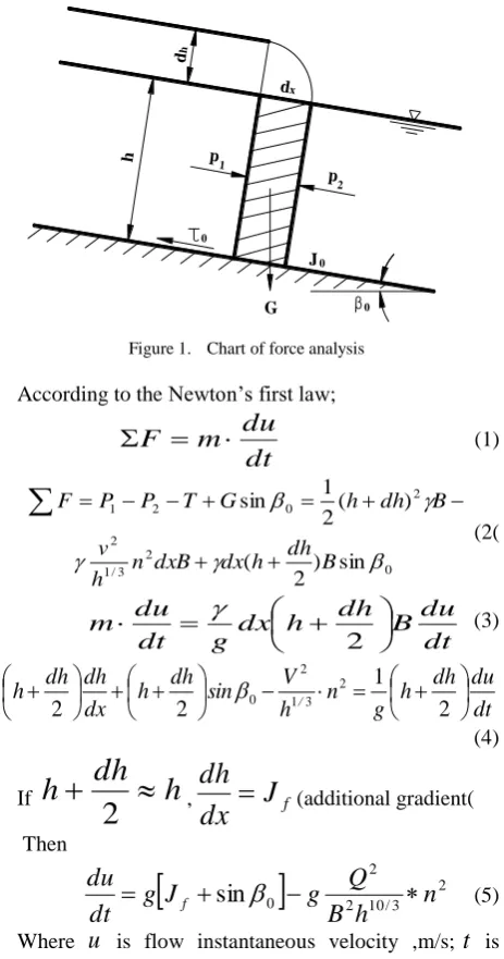
If B is the width of river, the force analysis of tiny flow stage can be seen in figure 1 [46,109].

dx dh h p 1 p₂ G J 0 0 0

Figure 1. Chart of force analysis

According to the Newton’s first law;

dt

du

m

F







(1)

0 2 3 / 1 2 2 0 2 1 sin ) 2 ( ) ( 2 1 sin      B dh h dx dxB n h v B dh h G T P P F         



(2(

dt

du

B

dh

h

dx

g

dt

du

m











 





2



₍₃₎

dt du dh h g n h V sin dh h dx dh dh

h _/ 

                        2 1 2 2 2 3 1 2 0



(4)

If

h

dh

h





2

,

dx

J

f

dh

_

(additional gradient(

Then





_{2 10/3} 2

2 0

sin

n

h

B

Q

g

J

g

dt

du

f











(5)

Where

u

is flow instantaneous velocity ,m/s;

t

is time,s;g is gravity acceleration,m/s2 ;

J

_f is additional gradient; ₀ is river bottom slope angle;h is average depth,m;

n

is comprehensive roughness of river.

Seen from the equation5, the influence factors on the flow acceleration includes;

(1(slope increase (2(roughness reduce(3(de-siltation is narrow and deep.

Additional gradient refers to the difference value of the water surface slope with 1-d uniform flow water surface slope. If in a very short period of time, the horizontal displacement is



x

, vertical displacement is



y

, then the additional gradient can be calculated as followings.

J

_f

y

x







(6(

So, to a water particle, if the water level can change

from

Z

₁ to

Z

₂ during the time from t1 to t2, the distance

1 2 1 2 1 2 1 2 t t X t t Z Z X Z Z J        

 (7)

Usually, velocity in surface water is close to the maximum measured velocity

max 1 2

V

t

t

X

_





₍₈₎

Where

V

_max is the maximum velocity, so the additional gradient can be calculated as followings

max 1 2 V t Z Z J   

 (9)

Comparison with the gradient of river, additonal gradient was small. Using measured data, according to the above equation, additional gradient in huayuankou station in “04.8” flood is -0.18o_/ooo, Even if in the

maximum flood, the additional gradient only 0.082 o_/ooo.

That is to say, the influence of additional gradient on velocity is small , while in low silt-laden water , the influence of additional gradient on velocity is smaller.

III. EXPERIMENT STUDY

A. Experiment Instructment

The experiment is done in steel glass channel in Yellow River Institute of Hydraulic Research with rectangle profile, length of 22 meter , width of B=0.3m, height of H=0.5m,and roughness of n=0.010,slope of river bed of i=1/1000 and 3.8/1000. To ensure stability and uniformity, 10 meter at center is selected as experimental paragraph, electromagnetic flow meter is used to measure flow and rotor current meter is used to measure velocity. The channel test system can be seen in figure1.

Figure 2. Sketch of flume

B. Test Conditions

In the experiment, water depth is strictly controlled to make uniform flow in order to compare roughness coefficients in conditions of different sediment concentration. The experiment parameters is supposed as table1. TABLE I. EXPERIMENT PARAMETERS s



d/mm J (%) S /(kg.m -3 ) Q /(L.s -1 ) H /cm B/h Scope Medium

radius 2.65

0.0001-0.1 0.0080

0.1-0.38 2.5-402 20-30

9.5-20 1.5-3.15

C. Procedure of Experiment

To compare the backdrop of different sediment particle size, sediment concentration, flow conditions, the flow velocity distribution and sediment concentration along the vertical distribution, in accordance with the following steps to test.

(1) Open circulatory system to regulate the flow, water depth, to make uniform flow;

(2) Ensure that the cycle long enough time to allow more uniform blending of water and sediment, with flow meter for measuring sediment-laden flow velocity, while sampling, measurement of sediment concentration and sediment particle size distribution;

(3) Changes in sediment concentration or changing the flow rate or water depth, repeat steps (2)

(4) The group after the end of the experiment, washing sink and the circulatory system, and change the sediment on to the next set of experiments.

D. Determination of Roughness Coefficient

Water resistance can be usualy expressed by drag coefficient which can have different means of expressions including Chezy coefficient

C

and the Manning coefficient

n

and Darcy-Weesbach drag coefficient

f

.

)

/

22

.

12

lg(

3

.

2

8

6 / 1 3 / 1 6 / 1 s

k

R

g

kR

g

f

R

C

R

n











(10) Where

R

-hydraulic radius corresponding to Sand

resistance;

g

-gravity Acceleration;

k

_s- Bed roughness

IV. ANALYSIS OF EXPERIMENT

A. Velocity Distribution

Velocity distribution of viscous sublayer can be

expressed as

u





y

 , actual thickness of viscous

sublayer



_s is the distance of the intersection of viscous sublayer and transition layer to the zero. From the figure of the time average velocity, the upper point in line with

 

_

y

u

, the value of

y

is



_s. Equation of velocity

distribution is

*

1

ln(

)

_f

s

u

y

B

0 5 10 15 20 25

1 10 100

y+

u+

S=0 S=30 S=42 S=100

Figure 3. Velocity distribution of viscous sublayer

In this paper, using test algorithms, the greatest correlation coefficients can be got by turbulent zone boundaries. Using this method, the value of A and C calculated can be ensured the accuracy of, otherwise, an accurate value would be difficult to find.

The C value of rough bed is the maximum in rough bed, which is due to the smaller rough bed surface friction velocity.

B. Roughness Regular

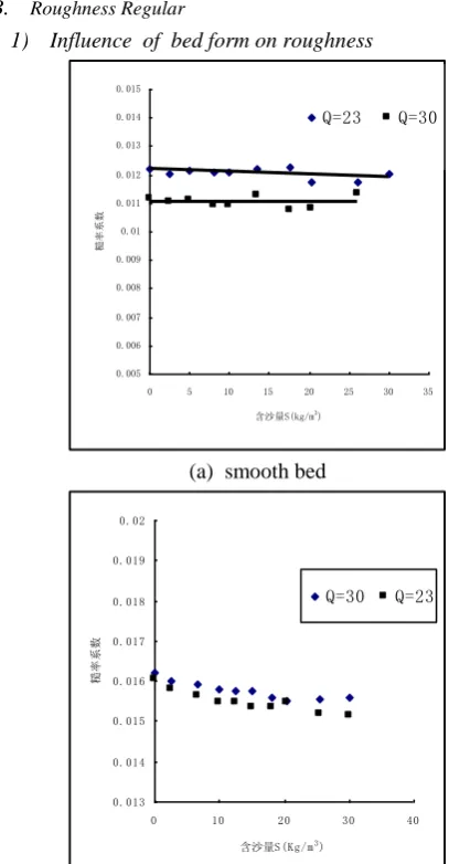
1) Influence of bed form on roughness

0.005 0.006 0.007 0.008 0.009 0.01 0.011 0.012 0.013 0.014 0.015

0 5 10 15 20 25 30 35

含沙量S(kg/m3

)

糙率系数

Q=23 Q=30

(a) smooth bed

0.013 0.014 0.015 0.016 0.017 0.018 0.019 0.02

0 10 20 30 40

含沙量S(Kg/m3₎

糙率系数

Q=30 Q=23

(b) adding coarse bed

0.013 0.0135 0.014 0.0145 0.015 0.0155

0 50 100 150 200 250 300

S

n

(c) rough bed

Figure 4. The influence of bed shape on roughness

Figure 4 for different bed get out of bed surface roughness curve with the sediment, in the smooth concrete surface and in the smooth concrete surface roughness of the bed form, there is the phenomenon of drag reduction, but not obviously, in the rough bed surface, roughness coefficient decreases with the increase of sediment concentration. When the concentration exceeds 50-60kg/m3, roughness increases with the concentration. While the rough bed was filled with fine sand, roughness reduces obviously, which indicate that the exchange of bed material plays an important role in the process decreases in the roughness

At present, there is no uniform understanding to the drag reduction, but the more influential topic is “secondary vertox”. To the smooth bed, the secondary vertox can noe be formed, so it is not obvious in drag reduction. To the rough bed, the bed can be seen as “V” bed, which can be easy form secondary vertox

2) Influence of sediment concentration on roughness coefficient

V. CHAOTIC BP NEURAL NETWORK MODEL

A. Phase-space Reconstruction

Time delay embedding phase space reconstruction method is the basis for dealing with non-linear time series. The principle is that the attractor is got in phase-space from one-dimensional time series reconstruction. Thus dynamics characteristic of reconstructed attractor analysis system is used. Takens theory holds that dynamic information of any one system is contained in a variable time-series of the system. State trajectory obtained when the single variable time series is embedded in a new coordinate system retains the main features of original phase- space state trajectory.

Specific ideas are as follows:

Assuming that time series{ ( ),x n n1, 2,..., }N _{is the} output variable in system

( 1)

[ ,

, ,

]

i i i i m

Y



x x

_

x

_{  }

Where

i



1 , 2 ,

,

N

m_,

N

m



- ( -1)

N

m



_is the number of reconstruction vector, m is the dimensional number,



is delay constant which is integer; this kind of method that the state vector is obtained from time series { ( ),x n n1, 2,..., }N is called as time delay embedding.

It is important to select time delay and embedding dimension m in the reconstruction.

Its accuracy is directly related to the accuracy of the invariant characteristics of strange attractors after phase-space reconstruction. From the experimental or measurement system under test signal through the delay embedding method will really reflect the dynamic characteristics of the system, you must carefully select the embedding dimension and time delay constant

3 Chaos Recognition

Whether a system is a chaotic system or the existence of chaotic elements, there are two characteristic parameters commonly used in criterion. One is the attractor dimension, the other is maximum Lyapunov index. Fractal dimension characteristics of attractor are the fundamental characteristics of chaos. Grassberger and Procaccia firstly proposed correlation dimension calculation method of attractor dimension from the experimental data, which is called as GP method. Correlation dimension of white noise increases with the embedding dimension increasing, while the correlation dimension of chaotic signals is convergence with the embedding dimension increasing, the dimension of convergence is called as dimension of attractors. Therefore, correlation dimension is used as a distinction between chaos and white noise. However , in subsequent studies, white noise is found to be shown the convergence characteristics. So , it is not enough only the correlation dimension as a criterion. People found that the fundamental characteristics of chaos manifested the extreme sensitivity to the initial value. The sensitivity is often used a different initial yapunov index to measure, Lyapunov index reflects initial orbit close to the

divergence of velocity. The size, positive and negative of Lyapunon index reflects the stretch and contraction in all directions. Correlation dimension of flood time series appeared a saturation with the embedding dimension increasing. So flood system has chaos characteristics.

B. BP neural network

An artificial neural network (ANN), also called a simulated neural network (SNN) or commonly just neural network (NN) is an interconnected group of artificial neurons that uses a mathematical or computational model for information processing based on a connectionistic approach to computation. In most cases an ANN is an adaptive system that changes its structure based on external or internal information that flows through the network.

In more practical terms neural networks are non-linear statistical data modeling or decision making tools. They can be used to model complex relationships between inputs and outputs or to find patterns in data.

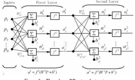
In recent years, neural network has been widely applied to the different scope, in which BP network is commonly used. The model created in this paper is a BP neural network with three-layer network (Figure5),

Figure 5. Three-layer BP network structure

In the Figure 1,

p

is input of neuron. Each layer has

its own weight matrix

W

, its bias vector

b

, a net input

vector

n

, and an output vector

a

.

W

is an

S



R

matrix, and

a

and

b

are vectors of length

S

respectively. The superscripts of symbols identify the

layers. Also shown in Figure 1 are

R

input,

1

S

_neurons

in the first layer, and

S

2 neurons in the second layer. Different layers can have different numbers of neurons. The outputs of layers one and two are the inputs for layers two and three. Thus layer 2 can be viewed as a

one-layer network with

R



S

1inputs,

S



S

2 neurons, and an

S

1



S

2 weight matrix

1

W

_{. The input of layer 2}

is

1

a

_{, and the output is}

a

2_{. The other layer also can be} drawn using same abbreviated notation.

i i ji

i

w

y

s









(11)

Several types of transfer functions are used; however, the most frequently used is the sigmoid function. This transfer function is usually a steadily increasing S-shaped curve. The sigmoid function is continuous, differentiable everywhere, and monotonically increasing. In this study, two S-shaped transfer functions in a MATLAB neural network toolbox were used: the tansig function and logsig function. The two functions are of the form:

1 1

2 ) (

tan ₂ 

  _{ n}

e n

sig (12)

n e n

sig _

 

1 1 ) (

tan (13)

These accumulated inputs are then transformed to the neuron output. This output is generally distributed to various connection pathways to provide inputs to the other neurons; each of these connection pathways transmits the full output of the contributing neuron. Second, the error between the real output and the expected output will be computed. If the expected error is not satisfied, the precision, weights and biases will be adjusted according to the error.

.

Figure 6. Flowchart of BP neural networks algorithm

C. Application

Determination of input pattern is the key to an excellent neural network. Too few or too many input nodes can affect either the learning or prediction

capability of the network. Therefore, we use input variables and the lag time as the input to make forecasts for future values. Since there are no suggested systematic ways to determine the appropriate number of neurons, the best way to select input variables is by trial-and-error. Median grain size of bed load, sediment concentration, median grain size of suspended load, Froude number is the input of the model, the flood water level is the output of the model. We develop a model for the RBF algorithms (Figure 3)

lower

H

=

f

{

d

_b50,

S

,

d

_s50,

H

_upper } Where

d

_b50- median grain size of bed load;

S

-sediment concentration;

d

_s50- median grain size of bed load;

When the number of hidden layers are 6, the model is stable and can get the ideal result. The structure of topology is 4-6-1. For better performance in our experiments, we use a small learning rate of 0.10 and the associated momentum factor of 0.95 in the training, the expired error is 0.0001

Figure 7. Structure of RBF neural networks of roughness coefficient

The number of input layer can be adopted as 4, hidden layer is 5,output layer is 1,the structure is 4-6-1.

Dimsize is 141, popsize is 25,

4

.

0

,

9

.

0

_min

max



w



w

,

c

1



c

2



2

,MSE is 1e-5. the

0 500 1000 1500 2000 2500 3000 3500 4000

06-7-27 06-8-1 06-8-6 06-8-11 06-8-16

data

Q

(m3

/s

)

calculated data

observation data

Figure 8. Observed data and calculated data in Huyuankou Station

0 500 1000 1500 2000 2500 3000 3500

06-7-22 06-8-1 06-8-11 06-8-21 06-8-31 06-9-10 06-9-20

Data

Q(m

3/s)

calculated data observation data

Figure 9. Observed data and calculated data in Jiahetan Station

0 1000 2000 3000

2006-7-30 2006-8-2 2006-8-5 2006-8-8 2006-8-11 2006-8-14 2006-8-17

日期

流量/

m

3/s

实测值 计算值

Figure 10. Observed data and calculated data in Gaocun Station

VI. CONCLUSION

Flood peak increase is caused by roughness decrease. Chaos BP neural network model is a mathematical methodology which describes relations between the input and output data irrespective of processes behind and without the need for making assumptions considering the nature of the relations. They are dependent on the particular samples observed and require tedious

experiments and trial-and-error procedures. However, several distinguishing features of ANNs – adaptability, nonlinearity, and arbitrary function mapping ability – make them valuable and attractive tools for simulations of complicated hydrologic processes. The comparison study of ANN with measured roughness coefficient indicates that ANN performs well on the flood water level calculation.

ACKNOWLEDGMENTS

This study was funded by the National Basic Research Program of China (2010CB951101), the National Natural Science Foundation of China (Grant No. 40830639, 50879016, 50979022 and 50679018), the program for Changjiang Scholars and Innovative Research Team in University (IRT0717) and the Special Fund of State Key Laboratory of Hydrology-Water Resources and Hydraulic Engineering (1069-50985512, 1069-50986312)

REFERENCES

[1] Qian Ning. Hyper-concentrated Flow [M].Beijing:

Tsinghua University Press,1989.

[2] Yang,S.-Q,Tan S.-K.,and Lim S.-Y.(2004).Velocity

Distribution and Dip-Phenomenon in Smooth Uniform Open Channel Flows. J.Hydraul. Eng., 130(12):1179-1186. [3] Chiu C.-L., Jin W.-x., and Chen Y.-C. (2000). Mathematical Models of Distribution of Sediment Concentration. J.Hydraul. Eng.,126(1):16-23.

[4] Chiu C.-L.(1989) Velocity Distribution in Open Channel Flow. J. Hydraul. Eng,115(5):576-594.

[5] Liu C.J.,Li D.S.,Wang X.-K.(2005). Experimental study on friction velocity and velocity profile of open channel flow. J.Hydraul. Eng.,36(8):950-955.(in Chinese)

[6] Fei Xiangjun. Resistance of Homogeneous Flow with

Hyperconcentration and Problem of “Resistance

Reduction” in Turbulent Regime[J].Journal of Sediment Research,1985(1):13-21.

[7] Lian Jijian, Hong Roujia. Turbulence Characteristics of Drag-reducing flows with muddy meds [J]. Journal of Hydraulic Engineering,1995,(9):13-21.

[8] Wang Zhaoyin, Song Zhenqi. The Phenomenon of Drag Reduction in Flows of Clay Suspensions[J]. Acta Mechanica Sinica,1996,28(5):522-531.

[9] Shu Anping, Liu Qingquan,Fei Xiangjun. Unified Laws of velocity Distribution for sediment laden flow with high and

low concentration[J].Journal of Hydraulic

Engineering,2006,37(6)1175-1180.(in Chinese)

[10]Zhang Dao-cheng. Preliminary Study on the Rheological Parameters of Bingham Fluid in Laminar and Uniform Open Channel Flow[J]. Journal of Chengdu University of Science and Technology,1990(1):89-96.(in Chinese) [11]Xia Dehong, Zhou jun, Wu jie. The Drag Reduction

Mechanism and Measures for Pipe Flow of Bingham fluid [J]. Energy for Metallurgical Industry, 2002,21(1):31-34.(in Chinese)

[12]Qian Ning. Hyper-concentrated Flow[M].Beijing:

Tsinghua University Press,1989.

[14]Nezu, I. and W. Rodi (1986). Open channel flow measurements with a Laser Doppler Anemometer, J . Hydraulic Engineering, ASCE. , Vol. 112(5):335 - 355. [15]Song, T. C. and W. H. Graf (1994). Non - uniform open

channel flow over a rough bed. J . Hydro-science and Hydraulic Engineering, Vol. 12 (1) :1 - 25.

[16]Vanoni VA. Some effect of suspended sediment on flow characteristics. In: Proc. 5th Hydr. Conf. Bulletin 34,State Uni. of Iowa Studies in Engineering, Iowa, USA , 1953. [17]Chanson H, Qiao G. Drag reduction in hydraulic flows.

Proceedings of 1994 International Conference on Hydraulics in Civil Engineering, Brisbane, Australia, 1994,123~127.

[18]Lyn D.A. Resistance in flat bed sediment laden flows J of Hydraulic Engineering, ASCE, 1991, 117(1) : 94-114. [19]Hou H, Yang X1 Effect of fine sediment on the drag

reduction in muddy flow. In: Proc. of the Second International Symposium on River Sedimentation1 Nanjing: Water Resources and Hydraulic Power Press, 1983, 47-80.

[20]Wang Z. Y, L arsen P, Xiang W. Rheological properties of sediment suspensions and their implications. J. of Hydraulic Research, IAHR, 1994 (4) : 495~516-

[21]Wang Z Y, Ren Y.M , Wang X.K. Total pressure probe for the measurements of turbulence in sediment-laden flows. In: Proc. of 2nd International Conference on Hydroscience and Engineering, Beijing, Tsinghua University Press, 1995, 1875-1882.

[22]Graf WH, A ltinakar M. Hydraulique Fluviale. Lausanne: Presses Polytechniques et Universitaires Romandes, 1993.

Changjun Zhu received his B.S. in China University of Petroleum in 1999 and M.S. in the Chinese Academy of science, in 2002. Since then, he is the

lecturer of Hebei University of

Engineering from 2002 to present. Now he has received Ph.D. in the College of Hydrology and Water Resources, Hohai University in Nanjing, China, His main research interests are in numerical environment modeling.

Zhenchun Hao received his B.S. and M.S. in the College of Hydrology and Water Resources, Hohai University in Nanjing, China, in 1981 and 1984, respectively. He continued his education at the same university where he received a Ph.D. in hydrology in 1988. Now he is a professor of hydrology at the College of Hydrology and Water Resources, Hohai University in Nanjing, China. His research interests

include large-scale hydrological modeling, watershed