Approximation Of Randomized Block Design Towards Fuzzy Multiple Linear Regression: A Case Study In Health Sciences

(1)

Approximation Of Randomized Block Design

Towards Fuzzy Multiple Linear Regression: A

Case Study In Health Sciences

Wan Muhamad Amir W Ahmad, Soban Q. Khan, Rabiatul Adawiyah Abdul Rohim, Nor Azlida Aleng, Farah Muna Mohamad Ghazali

Abstract: ANOVA also provides a method of data analysis that is motivated by consideration of the experimental design or Design of Experiment (DOE). In this paperwork, a new dimension of the methodology by involving fuzzy regression approach to randomized block designs will be introduced, which is involving qualitative predictor variables under consideration on multiple linear regression. The idea from this research will be a useful thread for establishing comprehensive connectivity between randomized block designs and regression. The researchers can conclude that fuzzy MLR can predict much better compared to MLR itself.

Index Terms: Qualitative predictor variables, ANOVA, Design of Experiment, New Dimension, Multiple Linear Regression, Randomized Block Designs and Fuzzy Linear Regression

——————————  ——————————

1. INTRODUCTION

ANOVA was developed by Sir Ronald Fisher in the 1920s [1]. Analysis of variance (ANOVA) is a method of comparing the means of the response variable across different groups specified by the factor variable [2], [3]. On the basis of the statistics, ANOVA also provides a method of data analysis that is motivated by consideration of the experimental design or Design of Experiment (DOE). The design of an experiment should be determined by the scientific question that is being addressed and be balanced by the practicalconstraints of the experimental system [4]. According to the linear point of view, ANOVA can explain the nature of the statistical relation between the mean response and the level(s) of the predictor variable(s). This paperwork emphasized the methodology building from ANOVA to multiple linear regression and to fuzzy multiple linear regression. Through this methodology, we are trying to prove and validate the linear model results are equivalent to single-factor ANOVA.

First, let we consider the single-factor ANOVA model which given as followsY_ij  μ_. ε_ij, where;

Y

_ij = is the value of the response variable in the j th trial for i th factor level or treatment,

i



= are parameters,



_ij= are independent N(0,



2) with

n

j

i



1 ,



,

t

;



1 ,



,

. Let us determine the treatment means

as



_i then it can assume that



_i





_.







_i





_.



. The

difference can be denoted as



_i





_i





_.. The difference

.





_i



_i



is called the ith is factor level effect. So that, the ANOVA can be expressed as:

Y

_ij





.





_i





_ij, where



. = is a constant component common to all observations,



_i = is the effect of the ith factor level are independent [5].

Definition of

μ

_.

Let us define



_. be the unweight average of all factor level

means



_. with

t

i i

/

1 .







. This definition implies

0

1





 t

i i



because by



_i





_i





_.. So, we have





0

1

. 1













 



t

i i t

i



t





Then, we also have

t

i i

/

1 .







, so,



t



_.

t

i i





.

The ANOVA model which is given by

Y

_ij





_.





_i





_ijis called a factor effects model because it is expressed in terms of the factor effects



_i. To state ANOVA as a linear regression

model; we need to signify the parameters



_.

,



₁

,



,



_t in the

linear regression model. However, constraint

0

1





 t

i i



implies that one of the t parameters



_t is not needed since it

can be expressed in term of the other

t



1

parameters. We

shall drop the parameters



_i as

follows



_t







₁





₂





₃









_t_₁. Thus, we shall use only the parameters



_.

,



₁

,



,



_t_₁ for the linear model. For example, we now consider a linear regression model developed from single-factor of ANOVA. Consider a single ————————————————

 Wan Muhamad Amir W Ahmad, School of Dental Sciences, Health Campus, Universiti Sains Malaysia, Malaysia. E-mail: [email protected]

 Soban Qadir, School of Dental Sciences, Health Campus, Universiti Sains Malaysia (USM), 16150 Kubang Kerian, Malaysia. E-mail: [email protected]

 Rabiatul Adawiyah Abdul Rohim, School of Dental Sciences, Health Campus, Universiti Sains Malaysia, Malaysia. E-mail: [email protected]

 Nor Azlida Aleng, School of Informatics and Applied Mathematics, Universiti Malaysia Terengganu (UMT), Terengganu, Malaysia. E-mail: [email protected]

(2)

1304 study with

r



5

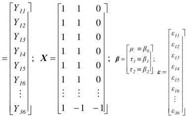
factor levels whenn1n2n34.

The

Υ,

Χ,

β

, and  matrices for this case are as follows:

(1)

Note that the vector of expected values,

Ε

 

Υ



Χβ

, yields the following equation:

From the calculation above, we can see that the above equation we can see that

E

 

Y

₁₁



μ

_.



τ

₁ it is equivalent as

 

Y

11

β

0

β

1

E





and the same process goes to all cells. The expected function for the last cell is given by

 

Υ

44

β

0

β

1

β

2

β

3

β

4

β

5

Ε





,

it is equivalent as

 

Υ44 μ. τ1 τ2 τ3 τ4 τ5

Ε       .

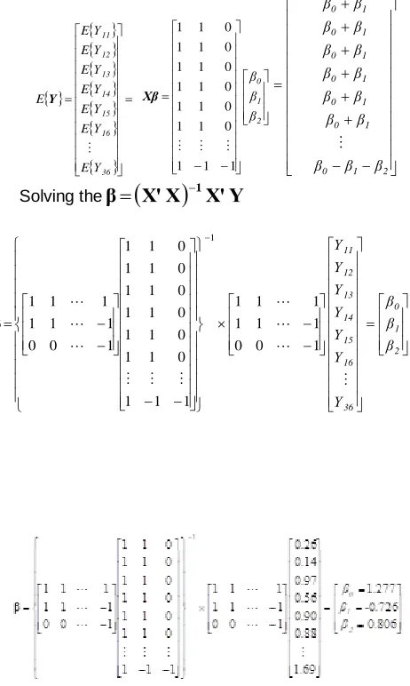
The next step is we calculate the estimated parameter of β by using the method of least squares as stated below. In, the matrix terms are

Χ'

Χβ



Χ'

Υ

. To obtain the estimated regression coefficients from the normal equation,

Υ Χ' Χβ

Χ'  by matrix methods, we premultiply both sides by the inverse of

Χ'

Χ

. It can be shown as



Χ'

Χ



1

Χ'

Χβ



Χ'

Χ



1

Χ'

Υ



with



Χ'Χ



1Χ'ΧΙ.

Solving that, we obtained the equation as β_



Χ'Χ



1Χ'Υ_. The illustration in (1) points out the general of multiple regression models so that it is equivalent of the single-factor ANOVA model,

Y

_ij





.





_i





_ij. The utmost important part of performing the regression approach to the single-factor analysis of variance is the coding requirement. In this stage, we require indicator variables that take on values 0, 1, or -1. The coding process should be done very carefully because it leads to the regression coefficient in the



vector that are the parameters in the factor effects ANOVA model, i.e.,

1 .

,



i

,



i





. Let Χ_ij₁ denote the value of indicator variable

1

Χ

. For the jth case from the ith factor level, Χ_ij₂ the value of indicator variable

Χ

₂ for this same case, and so on, using

altogether t-1 indicator in the model. The multiple regression model then is as follows:

ij t ij t ij

ij ij

ij



































_. ₁ ₁ ₂ ₂ ₃ ₃



_₁ _,_₁ (2)

where

otherwise

0 level

factor

from

case

if

1

1 level

factor

from

case

if

1 X

ij1





t



otherwise

0 level

factor

from

case

if

1

1 -level

factor

from

case

if

1 X

ij,t 1

t







In this case, the function parameters in (2) are linear in term of regression point of view; the intercept term is

μ

and the

regression coefficient is denoted as

τ

_i

,



,

τ

_i₁. To test the equality of the treatment means



_i by means of the regression approach, we state the null hypothesis as

1 2

1

0

:



t

H







and

H

₁

:

not all



_i are equal zero.

Thus, we can employ the usual test statistic

MSE MSR F for

testing whether or not there is a regression relation.

(3)

 

(

3 )

BMI



A

0



A

1

X

1



A

0

X

2

All independent variables need to be significant before we proceed the fuzzy regression analysis. Variable caries is not crisp but is instead fuzzy in nature. This implies that the parameter is also fuzzy in nature. Our aim is to estimate this parameter.

A

₁



a

₁_c

,

a

₁_w



and

A

₂



a

₂_c

,

a

₂_w



, where

1c

,

2c

a

is the center and

a a

₁_w ₂_w is radius or vagueness associated. The above fuzzy set describes the belief of regression coefficient around

a

_icin term of the symmetric triangular membership function. It is also to be noted that the methodology is applied when the underlying phenomenon is fuzzy which means that the response variable is fuzzy and the relationship is also considered to be fuzzy. In fuzzy regression methodology, parameters are estimated by minimizing total vagueness in the model. From equation

1 1c

,

1w

A



a



and

A

₂



a

₂_c

,

a

₂_w



. From the equation (3), we can rewrite the equation as follows.

 

  

  

 

 _0c _0W _1c _1W ₁ _2c _2W ₂ _jc _jw

j a ,a a ,a X a ,a X BMI ,BMI

BMI

(4)

Thus,

(3a)

2j

2c 1j 1c 0c

jc

a

X

a

X

BMI





(3b)

2j

2w 1j 1w 0w

jw

a

X

a

X

BMI





w

BMI

represent radius and cannot be a negative value. The linear programming of the methodology can be expressed as follows.

Minimize











m

j 1

2j 2w 1j 1w

0w

a

X

a

X

a

(4) Subject to



 





a

0c



a

1c

X

1j



a

2c

X

2j



a

0w



a

1w

X

1j



a

2w

X

2j





BMI

j (4a)



 





a

0c



a

1c

X

1j



a

2c

X

2j



a

0w



a

1w

X

1j



a

2w

X

2j





BMI

j (4b)

and

a

_iw



0

.

2 NUMERICAL

EXAMPLES

For example, we now consider a linear regression model developed from single-factor of ANOVA. Table 1 gives the full dataset of the case study.

TABLE 1

DATA OF TRIGLYCERIDES READING ACCORDING TO SMOKING STATUS

Code: BMI= Body Mass Index

Code: deft =Caries Status : 1 = No caries; 2 : Low Caries , 3 : Moderate

Consider a single study with

r



3

factor levels whenn₁ n₂ n₃6.

TABLE 2

REGRESSION APPROACH TO THE ANALYSIS OF VARIANCE ANOVA

i j _deft

ij

Y BMI

Reading Xij1 Xij2

1 1 1 14.64 1.00 0.00

1 2 1 15.00 1.00 0.00

1 3 1 13.42 1.00 0.00

1 4 1 14.11 1.00 0.00

1 5 1 12.51 1.00 0.00

1 6 1 12.53 1.00 0.00

2 1 2 11.78 0.00 1.00

2 2 2 12.02 0.00 1.00

2 3 2 12.03 0.00 1.00

2 4 2 12.25 0.00 1.00

2 5 2 12.32 0.00 1.00

2 6 2 12.41 0.00 1.00

3 1 3 11.63 -1.00 -1.00

3 2 3 11.63 -1.00 -1.00

3 3 3 11.98 -1.00 -1.00

3 4 3 12.10 -1.00 -1.00

3 5 3 12.10 -1.00 -1.00

3 6 3 12.26 -1.00 -1.00

The

Υ,

Χ,

β

, and  matrices for this case are as follows:

;

          

 

          

 



36 16 15 14 13 12 11

Υ Υ Υ Υ Υ Υ Υ



Υ ;

1 1 1

0 1 1

          

 

          

 

  

  

Χ ;

  

 

  

 

   

2 2

1 1

0 .

β τ

β μ

β

) 1 (

          

 

          

 



36 16 15 14 13 12 11

ε ε ε ε ε ε ε



(4)

1306                                             36 16 15 14 13 12 11 Υ E Υ E Υ E Υ E Υ E Υ E Υ E E  Υ                                        2 1 0 β β β 1 1 1 0 1 1 0 1 1 0 1 1 0 1 1 0 1 1 0 1 1    Χβ                                    2 1 0 1 0 1 0 1 0 1 0 1 0 1 0 β β β β β β β β β β β β β β β 

Solving the

β





Χ'

Χ



1

Χ'

Υ

                                                                                                                      2 1 0 36 16 15 14 13 12 11 β β β Υ Υ Υ Υ Υ Υ Υ           1 0 0 1 1 1 1 1 1 1 1 1 0 1 1 0 1 1 0 1 1 0 1 1 0 1 1 0 1 1 1 0 0 1 1 1 1 1 1 1 β

The computer run of the multiple regressions of Triglycerides on X3 and X2 yielded the fitted regression function and analysis of variances table presented in Table 3

SAS Algorithm for Multiple Linear Regression

Data ANOVA;

Input BMI X1 X2; cards;

14.64 1.00 1.00 0.00 15.00 1.00 1.00 0.00 13.42 1.00 1.00 0.00 14.11 1.00 1.00 0.00 12.51 1.00 1.00 0.00 12.53 1.00 1.00 0.00 11.78 2.00 0.00 1.00 12.02 2.00 0.00 1.00 12.03 2.00 0.00 1.00 12.25 2.00 0.00 1.00 12.32 2.00 0.00 1.00 12.41 2.00 0.00 1.00 11.63 3.00 -1.00 - 1.00 11.63 3.00 -1.00 -1.00 11.98 3.00 -1.00 -1.00

12.10 3.00 -1.00 -1.00 12.10 3.00 -1.00 -1.00 12.26 3.00 -1.00 -1.00 ;

ods rtf file= "output.rtf" style= journal; Proc reg data=ANOVA;

model BMI = X1 X2; run;

ods rtf close; run;

Output

TABLE 3

PARAMETER ESTIMATES

Variable DF

Parameter Estimate

Standard

Error t -Value Pr > |t| Intercept 1 12.596 0.152 83.051 0.00

X1 1 1.106 0.214 5.157 0.00

X2 1 0.460 0.214 -2.146 0.04

The regression equation can be written as

2 1

0.460X

1.106X

12.596 BMI





2 1 2 1

X

214 .

0 ,

460 .

0 X

214 .

0 ,

106 .

1

52 12.596,0.1

X

error

Std

,

460 .

0 X

error

Std

,

106 .

1 error

Std

12.596,

BMI

































For the upper limit

2 1 2 1 X 674 . 0 X 32 . 1 748 . 12 X 214 . 0 460 . 0 X 214 . 0 106 . 1 0.152 12.596 BMI              

For the lower limit

2 1 2 1 X 246 . 0 X 892 . 0 444 . 12 X 214 . 0 460 . 0 X 214 . 0 106 . 1 0.152 12.596 BMI              

SAS Algorithm for Fuzzy Multiple Linear Regression

Title „Fuzzy Regression‟; Data ANOVA;

Input BMI X1 X2; Datalines;

(5)

run;

ods rtf file='result_ex1.rtf'; Proc optmodel;

set j= 1..18;

number BMI {j}, x1{j}, x2{j};

read Data ANOVA into[_n_]BMI x1 x2; Print BMI x1 x2;

number n init 18; var aw{1..3}>=0; var ac{1..3};

min z1= aw[1] * n + sum{i in j} x1[i] * aw[2] + sum{i in j} x2[i] * aw[3];

con c{i in 1..n}: ac[1]+x1[i]*ac[2]+x2[i]*ac[3]

-aw[1]-x1[i]*aw[2]- x2[i]*aw[3] <= BMI[i]; con c1{i in 1..n}: ac[1]+x1[i]*ac[2]+x2[i]*ac[3]+

aw[1]+x1[i]*aw[2]+x2[i]*aw[3] >= BMI[i]; expand;

solve; print ac aw; quit;

ods rtf close;

Output

The fitted model for fuzzy regression is

2

1 0.19333,0. 000 X

X 0.465 1.00167, 0.780

12.75333,

BMI    

For the fuzzy regression model, the prediction equations for the computing upper and lower limits, obtained are as follows. For the upper limit

2 1

0.19333X 1.46667X

13.5333

X 0.000 0.19333 X

0.465 1.00167 0.780

12.75333 BMI

 



  

    

   

For the lower limit

2 1

0.19333X 0.53667X

11.9733

X 0.000 0.19333 X

0.465 1.00167 0.780

12.75333 BMI

 



  

    

   

TABLE 4

COMPARISON THE ORIGINAL AND PREDICTED VALUE (95% CI) THROUGH THE MLR AND

FUZZY MLR

Original value

BMI

Predicted Value

MLR

Predicted Value Fuzzy MLR

Absolute Residual1

Absolute Residual2

14.64 13.70 13.76 0.94 0.88

15.00 13.70 13.76 1.30 1.24

13.42 13.70 13.76 0.28 0.34

14.11 13.70 13.76 0.41 0.36

12.51 13.70 13.76 1.19 1.24

12.53 13.70 13.76 1.17 1.22

11.78 13.06 12.56 1.27 0.78

12.02 13.06 12.56 1.04 0.54

12.03 13.06 12.56 1.02 0.53

12.25 13.06 12.56 0.80 0.31

12.32 13.06 12.56 0.74 0.24

12.41 13.06 12.56 0.65 0.15

11.63 11.03 11.94 0.60 0.31

11.98 11.03 11.94 0.95 0.04

12.10 11.03 11.94 1.07 0.15

12.26 11.03 11.94 1.23 0.32

14.64 13.70 13.76 0.94 0.88

15.00 13.70 13.76 1.30 1.24

13.42 13.70 13.76 0.28 0.34

14.11 13.70 13.76 0.41 0.36

12.51 13.70 13.76 1.19 1.24

Absolute Residual1:

e



y



yˆ

MLR Absolute Residual2:

FuzzyMLR

yˆ

y

e





The efficiency of the proposed method can be measured through absolute mean that obtained from the residual. The smallest mean value of residual indicates the better prediction of the results. Table 4 indicates the residual that obtained from our calculation. To determine which of proposed method the best is, the independent samples t-test was used to determine either the residual from MLR or fuzzy MLR is the smallest.

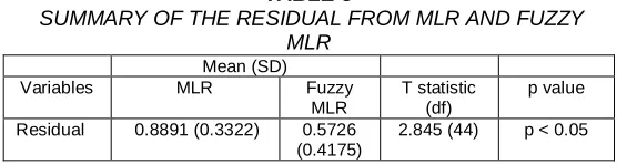
TABLE 5

SUMMARY OF THE RESIDUAL FROM MLR AND FUZZY MLR

Mean (SD)

Variables MLR Fuzzy

MLR

T statistic (df)

p value Residual 0.8891 (0.3322) 0.5726

(0.4175)

2.845 (44) p < 0.05

Since p = 0.007 < 0.05, the null hypothesis is rejected and the mean of residual can be concluded to be significantly different between MLR and fuzzy MLR. Therefore, we can say that the residual mean of fuzzy MLR 0.5726 (0.4175) is lower compared to MLR 0.8891 (0.3322). Therefore, this indicates that the fuzzy methodology of MLR is much better in giving the prediction compared to MLR.

3 CONCLUSION

The objective of this research is to build a methodology which can be used to predict the observation from randomized block design. Besides that, this methodology can be used as a tool for assessing the significant level of factor determination. According to the result that gained from section numerical example, we can conclude that fuzzy MLR can predict much better compared to MLR itself.

ACKNOWLEDGMENTS

The authors would like to express their gratitude to Universiti Sains Malaysia (USM) for providing the research funding (RUI Grant No.1001/PPSG/8012278, School of Dental Sciences, Kampus Kesihatan, Kelantan).

REFERENCES

[1] Armstrong, R. A., et al. .“An introduction to the analysis of variance (ANOVA) with

special reference to data from clinical experiments in optometry.” Ophthalmicand Physiological Optics 20(3): 235-241. 2000.

[2] Shahbaba, B. Analysis of Variance (ANOVA) Biostatistics with R (pp. 221-234; Springer. 2012.

(6)

1308 [4] Churchill, G. A.. Using ANOVA to analyze microarray

data. Biotechniques, 37(2), 173-177, 2004. [5] Neter, J., Kutner, M.H., Nachtsheim, C.J., and

Wasserman, W. Applied Linear Statistical Models. 4th Edition, WCB McGraw-Hill, New York, 1996. [6] Tanaka H., Uegima S., Asai K.,. Linear regression

analysis with the fuzzy model. IEEE Trans. Systems, Man and Cybernetics, 12, 903-907, 1982. [7] Bárdossy, A.. Note on fuzzy regression. Fuzzy Sets

and Systems, 37(1), 65-75, 1990.

[8] Kao, C., & Chyu, C.-L.. Least-squares estimates in fuzzy regression analysis. European Journal of Operational Research, 148(2), 426-435. 2003. [9] Kumar, A., et al.,.Fuzzy regression interval models for

forewarning onion thrips. Computing for Sustainable Global Development (INDIACom), International Conference on, IEEE, 2014.