STUDY OF COMPRESSIBLE FLUID FLOW IN BOUNDARY
LAYER REGION BY HOMOTOPY ANALYSIS METHOD
Achala L. Nargund1, R. Madhusudhan2 & S. B. Sathyanarayana3
1.INTRODUCTION
Compressible flow is having a wide applications in the field of mechanical and aerospace engineering, some of the applications includes nozzles and diffusers, turbines, fans, natural gas transmission lines and combustion chambers [1]. The Homotopy analysis method is applied to find an analytical solutions to non-linear equations and it was introduced by Liao in 1992 [2]. Homotopy Analysis Method is applied to discuss an approximate analytical solution of compressible boundary layer flow with an adverse pressure gradient by L. N. Achala and S. B. Sathyanarayana [3] . N. Curle [4] studied the functional relationships between the skin friction, pressure gradient and shape parameters, where in the effects of compressibility appearing explicitly in certain terms. T. Cebecci, A. M. O. Smith [5] studied numerically the unsteady laminar flow over a circular cylinder started impulsively from rest. N. Kafoussias, A. Karabis, M. Xenos [6] studied the two dimensional laminar compressible boundary layer flow over a flat plate with an adverse pressure gradient in the presence of heat and mass transfer numerically by Keller box method. G. Kuerti and A. D. Young [7, 8] have appropriately carried out an analysis in compresible boundary layers. More recent times the application of suction is also applied to remove separation and to reduce drag, studied by J. D. Anderson [9]. L. Howarth [10] studied extensively the separation and retardation of the laminar boundary layer equations. There were many numerical approaches discussed by T. Cebecci, P. Bradshaw and S. Schreier [12, 11]. M. Xenos, E. Tzirtzilakis and N. Kafoussias [13] studied numerically by Keller box technique the effects of blowing and suction on the steady compressible boundary layer flow with adverse pressure gradient and heat transfer over a wedge. Review of current ideas concerning unsteady boundary layer separation was studied by N. Riley [14]. By using quasi-linearization technique with an implicit finite difference scheme A. Sau and G. Nath [15] discussed numerical solutions of flow and heat transfer process on the unsteady flow of a compressible viscous fluid with variable gas properties over an infinite swept cylinder. The heat and mass transfer for unsteady laminar compressible boundary layer flow which is asymmetric with respect to a 3-dimensional stagnation point have been numerically solved using an implicit finite-difference scheme studied by Kumari. M and Nath. G[16].
In this work an attempt is made for studying the effects of the adverse pressure gradient on the separation of the compressible steady, two dimensional laminar boundary layer flow under the presence of a constant velocity of suction or injection at the wall. The methodology is presented in section-2, formulation of the problem is presented in section-3, while in section-4 the HAM solution is discussed. The Pade approximation is discussed in section-5. Results and graphs followed by an extensive analysis is done in section-6 and 7.
2.METHODOLOGY 2.1 Basic Idea Of HAM
Liao in 1992 [2] applied the Homotopy to solve nonlinear differential equations analytically. Consider the nonlinear differential equation
1 P. G. Department of Mathematics and Research Centre in Applied Mathematics, M. E. S. College of Arts, Commerce and Science, 15th cross, Malleswaram, Bangalore – 560003
2
Jyothy Institute of Technology, Tataguni off Kanakapura Road, Bangalore-560082. 3 Vijaya College, R.V Road, Basavanagudi, Bangalore-560004.
International Journal of Latest Trends in Engineering and Technology
Vol.(9)Issue(1), pp.028-039
DOI: http://dx.doi.org/10.21172/1.91.05
e-ISSN:2278-621X
Abstract-The partial differential equations governing compressible boundary layer flow problems cannot be solved as it is, many authors have solved these problems by reducing to ode’s. Falkner-Skan transformations will reduce the governing partial differential equations in to two non-linear partial differential equations. These equations are solved by HAM and the convergence of this is studied by using the Domb Sykes plot. The effect of suction and injection are studied on the velocity and temperature distribution and are depicted in a graph. It is also observed that for large values of suction and injection flow separation exists in boundary layer region. Pade approximation is also applied to HAM series solution which helped us to identify the singularities. Convergence is verified by plotting
h
curve for all the three cases suction, injection, and no suction for both velocity and temperature.0,
=
)]
,
(
[
u
x
y
N
(1)where
u
(
x
,
y
)
is an unknown function,x
andy
are two independent variables. Liao [17] in his work in 1997 introduced a non zero auxiliary parameterh
to construct a two-parameter family of equations and it is called as zeroth-order deformation equation
(
,
:
)
(
,
)
=
[
(
,
:
)],
)
(1
q
L
x
y
q
u
0x
y
qhN
x
y
q
(2)where
(
x
,
y
:
q
)
is an unknown function,h
0
is an auxiliary parameter which provides us a convenient way to guarantee the convergence of homotopy series solution,q
is the embedding parameter,L
is an auxiliary linear operator and)
,
(
0
x
y
u
is an initial guess. Whenq
=
0
, we have
(
x
,
y
:
0)
u
0(
x
,
y
)
=
0,
L
(3)According to the linear property of
L
i.eL
(0)
=
0
(Theorem-4.17) [18] and using the fact thatu
0(
x
,
y
)
satisfy the initial conditions which is shown in [19], [20] it is obvious that),
,
(
=
0)
:
,
(
x
y
u
0x
y
(4)When
q
=
1
, we have0,
=
)]
:
,
(
[
x
y
q
hN
(5)here
h
0
, we will get an equivalent equation which is exactly same as the original equation. Then the Maclaurin series solution is obtained by,
)
,
(
)
,
(
=
)
:
,
(
1 = 0
m m
m
q
y
x
u
y
x
u
q
y
x
(6)
0,
=
at
)
:
,
(
!
1
=
)
,
(
q
q
q
y
x
m
y
x
u
mm
m
(7)
)
,
(
x
y
u
m is called them
th order homotopy derivative of
(
x
,
y
:
q
)
. Forq
=
1
, the series (6) becomes).
,
(
)
,
(
=
)
,
(
=
1)
:
,
(
1 =
0
x
y
u
x
y
u
y
x
u
y
x
mm
(8)Differentiating equation (2)
m
times with respect toq
and then dividing bym
!
and finally settingq
=
0
, we get the followingm
th order deformation equation
u
m(
x
,
y
)
mu
m1(
x
,
y
)
=
hR
m(
u
m1),
L
(9)where
0,
=
at
)]
:
,
(
[
1)!
(
1
=
)
(
11
1
q
q
q
y
x
N
m
u
R
mm m
m
(10)
and
1.
>
1,
1,
0,
=
m
m
m
(11)By using Mathematica, the linear equation (2) can be solved.
2.2 Evaluation of h
To plot the
h
curve and to know the value of the convergence parameterh
, the following method is applied.2.2.1 Plotting the solution for h curves
The
h
curves are obtained by plotting partial sums of first few derivatives off
k(
t
)
against the parameterh
. The partialregion the solution will converge.
2.3 Domb Sykes plot
The radius of convergence of a power series is estimated using Domb Syke’s plot [3].
.
0 =
n n n
Z
C
(12)By applying D’Alembert’s ratio test, distance to the nearest singularity can be measured. Reciprocal of radius of convergence
can be known by fitting a straight line with an intercept as
Z
0. Domb and Sykes proposed plotting to know the radius ofconvergence and is given by
n n
C
C
1against
n n
C
C
1against
n
1
..
1
=
1 lim
n n
C
C
n
R
(13)
2.4 Pade Approximation
A power series in a Pade summation is replaced by a sequence of rational functions known as Pade approximants. When the Taylor series does not converge, the Pade approximant gives good approximation for the function compared to truncated Taylor’s series [21].
A Pade approximation of series is
.
=
=
=
)
(
0 =
0 = 0
= n
n M
n n n N
n N M n n n
Z
B
Z
A
Zp
Z
a
z
f
(14)where we choose
B
0=
1
without loss of generality.3. FORMULATION OF THE PROBLEM
Flow Diagram
Consider a two dimensional boundary layer flow of a heat conducting perfect gas with steady, compressible and no body force with Prandtl boundary layer assumptions,
(
v
)
=
0,
y
u
x
(15)
,
=
y
u
y
dx
dp
y
u
v
x
u
u
(16).
1
1
=
y
u
u
Pr
y
H
Pr
y
y
H
v
x
H
u
(17)The total enthalpy of the fluid defined for a perfect gas is defined by
2
=
2
u
TC
H
p
, Prandtl number is defined as the ratioof fluid viscosity over thermal conductivity,
is the coefficient of fluid viscosity. We will be having three equations (15),(16) and (17) with five unknowns
,u
,v
,H
andp
. By usingu
=
u
e(
x
)
and
=
e(
x
)
in equation (16),p
can be eliminated.,
=
dx
du
u
dx
dp
e e e
(18)e
represents the conditions at the edge of the boundary layer. Substituting (18) in (16).
=
y
u
y
dx
du
u
y
u
v
x
u
u
e e e
(19)
The boundary conditions along with transpiration velocity
v
w at the wall are),
(
=
),
(
=
0,
=
0,
=
u
v
v
x
H
H
x
y
w w (20)
,
=
),
(
=
,
u
u
ex
H
H
ey
(21)where
is the boundary layer thickness.The compressible Falkner-Skan transformation and stream function
is given by
(
,
)
,
(
,
)
=
(
,
),
)
(
)
(
=
0
dy
x
y
u
f
x
x
y
x
x
v
x
x
u
e e e e e e y
(22)Falkner-Skan transformation is applied for reducing the system of equations (15), (17) and (19) to four unknowns
,u
,v
and
H
. Stream function
is used to eliminate
,u
,v
which exactly satisfies (15) and is given by,
=
,
=
x
v
y
u
(23)using (22) and (23) the system of equations (17), (19) along with boundary conditions (20) and (21) is reduced to two equations for two unknowns
f
andS
.
(
)
,
1
=
)
(0,
=
),
(
=
0,
=
0,
=
0 21
v
x
dx
x
u
x
f
f
x
S
S
f
w w x e e e w w
(26)1,
=
1,
=
,
=
e
f
S
(27)
where
b
,c
,d
,e
,m
1
andm
2
are defined as follows
,
=
,
=
,
1
1
=
,
=
,
=
,
=
2 e e e e e eH
H
S
Pr
b
e
H
Cu
Pr
d
c
C
C
b
(28)
1
,
=
.
)
(
2
1
=
2 21
dx
du
u
x
m
m
dx
dx
m
e e e e e e
(29)Homotopy analysis method is applied to the system of partial differential equations (24) and (25), with the boundary conditions (26) and (27) along with the coefficients defined in the equations (28) and (29).
4. HAM SOLUTION
The concept of finding an analytical approximations for highly non linear differential equation by using HAM is given by [2]. For a given nonlinear differential equation (24)
,
=
)]
,
(
[
2 2 2 2 2 2 2 1 3 3
x
f
f
x
f
f
x
f
c
m
f
f
m
f
b
x
f
N
(30)where
N
is a nonlinear operator andf
(
x
,
)
is an unknown function. The zeroth-order deformation equation is given by
.
=
)
,
(
)
:
,
(
)
(1
2 2 2 2 2 2 2 1 3 3 0
x
f
f
x
f
f
x
f
c
m
f
f
m
f
b
hq
x
f
q
x
f
L
q
(31)Since the expression of the solution
f
(
x
,
)
is representing a polynomial, the auxiliary linear operatorL
[18] can be easily chosen as,
=
2 2 3 3
L
(32)with boundary conditions
1,
=
)
:
,
(
0,
=
)
:
,0
(
,
=
=
)
:
,0
(
x
q
f
F
x
q
F
x
q
F
w
(33)applying the given boundary conditions (26) and (27) for the chosen
L
by using the propertyLf
=
0
to (31), we get the initial guess approximation.
).
,
(
=
,0)
,
(
x
f
0x
F
(34)When q = 1, we have
).
,
(
=
,1)
,
(
x
f
x
F
(35)
Solution varies from the initial guess
f
0(
x
,
)
to the exact solutionf
(
x
,
)
as q increases from 0 to 1. Using (34) the Maclaurin series of F(x,
,q) with respect toq
reads.
)
,
(
)
,
(
=
)
,
,
(
1 = 0 k k kq
x
x
q
x
F
(36) where0,
=
at
)
:
,
(
!
1
=
)
,
(
q
q
q
x
m
x
m m k
(37))
,
,
(
x
q
F
is called the Homotopy Maclaurin series and (37) is called thek
th order homotopy derivative ofF
(
x
,
,
q
)
, for1
=
q
the homotopy series is given by),
,
(
)
,
(
=
)
,
(
=
,1)
,
(
1 =0
f
x
x
x
x
F
m m
(38)where
m(
x
,
)
is the unknown function to be determined.By using Leibnitz theorem, differentiating equation (31)
m
times with the embedding parameterq
, setting q = 0 and dividing by m!, we get
1
=
hR
(
x
,
),
L
m
m m m (39)where
1,
>
1
1,
0
=
m
when
m
when
m
(40)
,
'
)
(1
=
]
,
[
' 0 = 0 = 2 ' ' 1 1 0 = 2 ' 1 1 0 = 1 ' 1
r r k r k r r k r k m k k m m k k k m m k m mx
x
x
x
c
m
m
m
b
x
R
(41)with boundary conditions
0.
=
)
,
(
=
,0)
(
=
,0)
(
x
m'x
m'x
m
(42)
The linear equations obtained from (39) is used to estimate
m by using MATHEMATICA and the graphs are analysed for different parameters.Initial approximation
f
0(
x
,
)
is obtained by choosingF
(
x
,0,
q
)
=
=
f
w=
ax
satisfying the boundary conditions1
=
=
)
,
(
00
e
ax
x
f
(43)
1 2 30
=
f
f
f
f
f
(44)
Applying HAM to (25) the given nonlinear equation is
,
=
)]
,
(
[
2 12 3 3 2 2
x
f
S
x
S
f
x
S
f
m
f
d
f
f
d
S
e
x
S
N
(45)where
N
is a nonlinear operator andS
(
x
,
)
is an unknown function. We construct the homotopy for the equation (45)
,
=
)
,
(
)
:
,
(
)
(1
2 12 3 3 2 2 0
x
f
S
x
S
f
x
S
f
m
f
d
f
f
d
S
e
hq
x
S
q
x
S
L
q
s
(46)where the auxiliary linear operator is defined by
,
=
2 2
sL
(47)with boundary conditions
1.
=
)
,
,
(
,
=
=
=
)
,0,
(
x
q
Bx
S
S
x
q
S
w
(48)Using the property
L
s(0)
=
0
along with the boundary conditions (48) we get an initial approximation in terms ofS
0(
x
,
)
,
1)
(
1
=
)
,
(
0
e
Bx
x
S
(49)the Homotopy Maclaurin series of
S
(
x
,
,
q
)
is given by,
)
,
(
)
,
(
=
)
,
,
(
1 = 0 k k kq
x
x
q
x
S
(50)for the case of
q
=
1
, we get).
,
(
)
,
(
=
,1)
,
(
1 =
x
x
x
S
kk
(51)By using
0(
x
,
)
=S
0(
x
,
)
, the remaining values like
1,
2,
3 can be obtained. The HAM series solution for (25)is given by
1 2 30
=
S
S
S
S
S
(52)The equations (44) and (52) represents HAM series solution for velocity and temperature which are analysed graphically for
different parameters. The suction/injection velocity at the wall,
v
w(
x
)
=
f
w=
=
a
x
andS
=
S
w=
=
B
x
where
a
andB
are the suction/injection parameters which is assumed as constant which becomes a valid assumption in order to ensure that the flow with suction or injection at the wall satisfies the simplifying conditions which forms the basis ofthe boundary layer theory [22] for the case of heating the wall
(
S
w=
B
=
2)
. Also,v
w(
x
)
represents the velocity of suctionor injection at the wall according as
v
w(
x
)
<
0
orv
w(
x
)
>
0
respectively.5. PADE APPROXIMATION
,
1
1)
1.19899(
1)
1.85488(
1)
2.27578(
0.655089
2
3
(53)
We observe that there is a singularity at
=
1.82335
which is seen in Figure 16.,
1
1)
0.748136(
1)
0.496159(
1)
0.130078(
5.16772
2
3
(54)We observe that there is a singularity at
=
1.73924
which is seen in Figure 17.,
1
1)
0.220981(
1)
0.0333967(
1)
0.0242783(
6.82719
2
3
(55)We observe that there is a singularity at
=
5.92347
which is seen in Figure 18..
000000000
1.00000000
1)
0.0794144(
1)
0.0460149(
1)
0.0200454(
0.926419
2
3
(56)We observe that there is a singularity at
=
5.19074
which is seen in Figure 19..
000000000
1.00000000
1)
0.0794232(
1)
0.0459651(
1)
0.0200025(
0.926316
2
3
(57)We observe that there is a singularity at
=
5.19374
which is seen in Figure 20..
1
1)
0.0794055(
1)
0.0460647(
1)
0.0200882(
0.926522
2
3
(58)We observe that there is a singularity at
=
5.18776
which is seen in Figure 21.6. RESULTS AND DISCUSSIONS
In this paper we have applied HAM for the governing partial differential equations (24) and (25). Convergence is verified by plotting
h
curve for all the three cases suction, injection, and no suction for both velocity and temperature in figure 1 - 6. According to the graph the value ofh
=
0.001
is used to analyze the velocity and temperature distribution in boundary layer region by identifying flow separation with suction/injection effects.Flow separation exists for the far distance against an adverse pressure gradient when the speed of the object falls almost zero. The fluid flow takes the forms of eddies and vortices when the object is detatched from the surface. The solid objects travelling through a fluid will have viscous forces which is close to layer of the fluid in the solid surface [23]. The portion of the boundary layer is closest to the wall or leading edge where the flow direction is reversed then the boundary layer separation occurs. When the shear stress is zero, between the forward and backward flow a separation point is defined. At the separation point the overall boundary layer initially thickens suddenly and is then forced off by the reversed flow at its bottom. Suction is used to remove the boundary layer from the surface before it separates as the flow separation in the velocity profile. Boundary layer suction is a technique where an air pump is used to extract the boundary layer at the wing [24]. The drag can be reduced to improve the air flow where in the fuel efficiency is estimated as high as
30
percent. If the flow is laminar then the velocity of the air increases steadily as measurements are taken away from the surface. Boundary layer flow is disturbed from the layer of the surface which creates a low pressure region immediately behind the airfoil [23], where the drag is overall increased for the low pressure region. For the careful design and smooth surfaces many attempts have been made to delay the onset of this flow separation.varying from -5 to 5. It is worth mentioning here that when the heat transfer parameter
S
w
1
corresponds to a flow withheat transfer, where as when
S
w=
1
corresponds to a flow with no heat transfer between the wall and the fluid and this flow is called as adiabatic flow. In this paper we considered the value ofS
w=
B
=
2
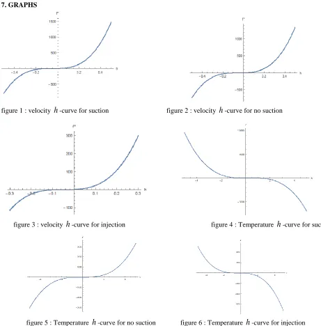
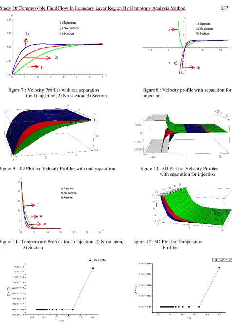
which corresponds to the case of heating the wall and the same is applied to the temperature profile for injection, no suction and suction which is presented in figure 11 and 12. To determine the radius of convergence for the HAM series solution Domb Sykes plot is presented in figure 13-15. To identify the singularities in the graph we have applied Pade for the HAM series solution (44) and (52) which is presented in Figure 16-21. The analytical results obtained in this paper are compared with the numerical results of [6] which shows good agreement for the velocity and temperature profiles with suction, injection and no suction effects. Achala and Sathyanarayana have applied HAM for this problem where the pressure is assumed constant across the boundary layer, therefore, the density can be assumed to be a function of temperature only, with this they are able to reduce the system of pde to ode where as we have applied directly to pde with out making any assumptions (2015)[3]. The important observation is that the existence of flow separation for injection which is not shown by previous authors.7. GRAPHS
figure 1 : velocity
h
-curve for suction figure 2 : velocityh
-curve for no suction
figure 3 : velocity
h
-curve for injection figure 4 : Temperatureh
-curve for suction
figure 7 : Velocity Profiles with out separation figure 8 : Velocity profile with separation for for 1) Injection, 2) No suction, 3) Suction injection
figure 9 : 3D Plot for Velocity Profiles with out separation figure 10 : 3D Plot for Velocity Profiles with separation for injection
figure 11 : Temperature Profiles for 1) Injection, 2) No suction, figure 12 : 3D Plot for Temperature 3) Suction Profiles
figure 15 : Domb-Sykes plot for suction with figure 16 : Pade velocity for no suction
R
=
0.596
figure 17 : Pade velocity for injection figure 18 : Pade velocity for suction
figure 21 : Pade Temperature for Suction
REFERENCES
[1] P.H. Oosthuizen, W.E. Carscallen, Compressible fluid flow, McGraw-Hill, New York, 1997.
[2] S.J. Liao, The proposed homotopy analysis techniques for the solution of nonlinear problems, Ph.D. dissertation, Shanghai Jiao Tong University, Shanghai, China, 1992.
[3] L.N. Achala, S.B. Sathyanarayana, Approximate analytical solution of compressible boundary layer flow with an adverse pressure gradient by homotopy analysis method, Theor. Math. Appl. 5(1) (2015) 15-31.
[4] N.Curle, The Laminar Boundary Layer Equations, Clarendon Press, Oxford,1962.
[5] T. Cebecci, A.M.O. Smith , Analysis of Turbulent Boundary Layers, Academic Press, New York, 1974.
[6] N. Kafoussias, A. Karabis, M. Xenos, Numerical study of two dimensional laminar boundary layer compressible flow with pressure gradient and heat and mass transfer, Int. J. Eng. Sci. 37 (1999) 1795-1812.
[7] G. Kuerti, The laminar boundary layer in compressible Flow, Adv. Appl. Mech. 2 (1951) 21-92.
[8] A.D. Young, Section on boundary layers, Int. J. Howarth (Ed.), Modern Developments in Fluid Mechanics High Speed Flow, Clarendon Press, Oxford, 1 (1953) 375-475.
[9] J.D. Anderson, Hypersonic and High-Temperature Gas Dynamics, McGraw-Hill, New York, 1989. [10] L. Howarth, Proc. Roy. Soc. London A 164 (1938) 547-579.
[11] T.Cebeci, P. Bradshaw, Physical and Computational Aspects of Convective Heat Transfer, Springer, Berlin, 1984. [12] S. Schreier, Compressible Flow, Wiley, New York, 1982.
[13] M. Xenos, E. Tzirtzilakis and N. Kafoussias, Compressible Turbulent Boundary-Layer Flow Control Over a Wedge, 2nd International Conference From Scientific Computing to Computational Engineering, 2nd IC-SCCE Athens, 5-8 July, 2006.
[14] N. Riley , Unsteady Laminar Boundary Layers ,Vol. 17, No. 2, April 1975.
[15] A. Sau and G. Nath, Unsteady compressible boundary layer flow stagnation line of an infinite swept cylinder, Acta Mechanica 108 (1995), 143-156. [16] M. Kumari and G. Nath (1980) Unsteady compressible 3-dimensional boundary-layer flow near an asymmetric stagnation point with mass transfer.
Int. J. 18 (11),1285-1300.
[17] S.J. Liao, A kind of approximate solution technique which does not depend upon small parameters (II), an application in fluid mechanics. Int. J. Nonlin. Mech. 32 (1997), 815-822.
[18] S.J. Liao, Homotopy analysis method in nonlinear differential equations, Springer, 2011.
[19] A. Sami Bataineh, M.S.M. Noorani, I. Hashim, Approximate analytical solutions of systems of PDEs by homotopy analysis method, Computers and Mathematics with Applications 55 (2008) 2913–2923.
[20] V.G. Gupta and Sumit Gupta, Application of Homotopy Aalysis Method For Solving Nonlinear Cauchy Problem, Surveys in Mathematics and its Applications, Volume 7 (2012), 105-116.
[21] C.M. Bender, S.A. Orszag, Advanced mathematical methods for scientists and engineers, McGraw- Hill International Book Company. [22] H. Schlichting, Boundary Layer Theory, Int. J. Kestin (Ed.), Trans., McGraw-Hill, New York, 1979.
[23] E.J. Shaughnessy Jr., I.M. Katz, J.P. Schaffer, Introduction to fluid mechanics, SI edition, Oxford University Press.