Petrasek

Forestry & Natural-Resource Sciences Last Correction: Aug. 11, 2010

A MONTE CARLO METHODOLOGY FOR SOLVING THE

OPTIMAL TIMBER HARVEST PROBLEM WITH STOCHASTIC

TIMBER AND CARBON PRICES

Stanislav Petr´

aˇ

sek

,

John Perez-Garcia

,

1_{Ph.D. Student,}2_{Professor, School of Forest Resources, University of Washington, Seattle, WA 98195 USA}

Abstract. This article presents a Monte Carlo methodology for solving the stochastic optimal timber

harvest problem modeled as a recurrent American call option. A detailed description of the proposed methodology is given, and the Monte Carlo technique is contrasted with finite difference methods typically used to find solutions of the optimal harvest problem with stochastic prices. The use of the methodology is then demonstrated via an example. In the example, expected bare land values and optimal harvest policies are calculated for a Douglas-fir stand in western Washington State. It is assumed that the forest owner derives revenue from traditional timber sales and carbon sequestration, and that prices of timber and carbon follow a known stochastic process. Results of the calculations are discussed.

Keywords:Optimal Harvest, Carbon Sequestration, American Option, Monte Carlo

1

Introduction

The optimal harvest problem is of fundamental impor-tance to forest economics and has been studied exten-sively for many years. A rich body of literature exists on determining the optimal harvest age and value of a for-est stand under different conditions. Traditionally, the analysis has been performed under the assumption that prices of timber are known and do not change over time. However, since the 1970’s, some researchers have been focusing their attention on the optimal harvest problem with stochastic timber prices.

One of the earliest articles to analyze the impact of stochastic timber prices on stand values and rotation lengths was presented by Norstrom 1975. This work was followed by other articles, for example those by Kaya and Buongiorno 1987 and Lohmander 1987. Arguments for an explicit treatment of stochastic timber prices and a review of existing literature were presented by New-man 1988, and New-many additional articles were published in the following decade. Among these were the articles by Morck et al. 1989, Haight 1993, and Plantinga 1998. A review of the existing literature on forest manage-ment in the presence of risk and uncertainty was given by Brazee and Newman 1999.

The articles by Morck et al. 1989 and Plantinga 1998 were two among several that analyzed the stochastic op-timal harvest problem using real options methodology,

an approach that applies ideas originally introduced in financial economics to the valuation and optimal man-agement of real assets under uncertainty.1 _{Two more} recent examples characteristic of the use of the real op-tions methodology in forest economics are the articles by Insley 2002 and Insley and Rollins 2005, who modeled the single and multi-rotation stochastic optimal harvest problems as American call options, a type of contract that gives its holder the right, but not the obligation, to harvest a forest stand at a given age. (For an introduc-tion to opintroduc-tions see, for example, the text by Hull 2003). Another recent example of a real options approach to risk management in forestry is provided by an article by Chladna 2007, who analyzed a stand management sce-nario where the forest owner receives revenue not only from timber but also from carbon emission permits.

Application of real option methodology to the stochas-tic optimal harvest problem typically yields a partial dif-ferential equation that must be solved numerically sub-ject to a set of conditions in space and time. Tradition-ally, the numerical solution techniques used in option valuation have employed finite difference schemes. The article by Insley and Rollins 2005 is perhaps the best example of this approach. Chladna 2007 did not specify the details of the methodology actually used to obtain the results of her study, but the partial differential

equa-1_{A thorough introduction to real options can be found in the} texts by Dixit and Pindyck 1994, and Trigeorgis 1996.

Copyright c2010 Publisher of the International Journal ofMathematical and Computational Forestry & Natural-Resource Sciences

tions that she derived could also be solved with finite difference schemes.

Finite difference methods are not the only methodol-ogy that can be employed in the valuation of real op-tions. As discussed, for example, by Glasserman 2004, a viable alternative is provided by algorithms based on Monte Carlo methods. From a theoretical perspective, the two approaches are equivalent in their ability to cal-culate option values. However, in the variety of problems considered in practical applications, some are more eas-ily solved with a finite difference scheme, while a Monte Carlo algorithm is a preferable choice for others.

The goals of this article are twofold. First, a Monte Carlo algorithm capable of solving the multiple rota-tion optimal harvest problem with two sources of uncer-tainty is presented. The algorithm is an adaptation of the method introduced by Ib´a˜nez and Zapatero 2004 for the valuation of financial American options, with modi-fications that extend the original method to infinite time horizons and multiple rotations. Second, the use of the extended algorithm is illustrated in a practical setting. The algorithm is used, in a scenario similar to that ana-lyzed by Chladna 2007, to determine the value and op-timal harvest schedule for a Douglas-fir site in western Washington State, under the assumption that the tra-ditional income from timber sales is supplemented by income from carbon sequestration.

The article is organized as follows. The logic of the re-cursive Monte Carlo method employed throughout the article is first introduced in Section 2 for the simplest case of a single-rotation, optimal harvest problem with stochastic timber prices. Section 3 introduces the case

withN >1 rotations and the modifications that are

re-quired before the method can be used to calculate bare land values and optimal timings in a multi-rotation set-ting. This is followed in Section 4 by a presentation of the multi-rotation method in the context of a stochas-tic optimal harvest problem with two sources of uncer-tainty. Finally, in Section 5, the two-dimensional, multi-rotation version of the method is applied to an illustra-tive problem, and the solution is presented and discussed in Section 6.

2

Wicksellian

Harvest

Problem

and

Monte Carlo

As discussed, for example, by Plantinga 1998 and In-sley 2002, the optimal timber harvest problem can be formulated as an American-style real option. The option formulation allows for the explicit treatment of stochas-tic timber prices, and it leads to harvest problem solu-tions in the form of expected bare land values and asso-ciated optimal harvest boundaries. These solutions are typically obtained with the use of various finite difference

methods. However, algorithms based on Monte Carlo methodology provide a flexible alternative for calculat-ing option values, of particular use in fields such as forest management, where the options of interest are charac-terized by multiple sources of uncertainty and complex payoffs and optimal harvest policies.

The Wicksellian (i.e., single rotation) optimal harvest problem with stochastic timber prices can be thought of as an American call option on the value of timber. It is particularly amenable to solution by Monte Carlo simulation, because it can be posed as the expectation maximization problem

π(S0, C) = sup

τ∗_∈R+E

[dτ₀∗Q_τ∗(S_τ∗ −C)+|S0, C], (1)

whereπ(S0, C) stands for the expected discounted value of a harvest that will take place at a future date for given values of harvest cost C and starting price S0, the supremum is taken over the harvesting times that assume values in the set of positive reals R+_{, τ}∗ _{is the} optimal harvest time,E[·|·] represents the conditional ex-pectation operator,dτ∗

0 is the discount factor from time τ∗ to present, Q_τ∗ denotes the timber volume specified

by the yield function Q_t at the optimal harvest time τ∗, and S_τ∗ denotes the stochastic price of timber per

unit volume. The term (S_τ∗ −C)+= max[S_τ∗ −C, 0]

and indicates that the stand is never harvested in peri-ods when harvest cost exceeds timber price. Equation 1 states that in order to maximize the profit from a sin-gle harvest, a forest owner must maximize the expected discounted harvest profit by selecting harvest time in response to price fluctuations.

The expected present value of harvest π(S0, C) in Equation 1 can be approximated by a Monte Carlo al-gorithm introduced by Ib´a˜nez and Zapatero 2004. As is the case with all American-style options, the algo-rithm produces a solution that consists of both the op-tion value π(S0, C) and the associated optimal harvest boundary B_t, which determines the minimum harvest price at which the stand should be harvested.

Several assumptions must be made before the Ib´a˜nez and Zapatero 2004 algorithm can be applied to the single rotation optimal harvest problem with stochastic tim-ber prices. The first of these assumptions concerns the treatment of time. Although time is assumed to be con-tinuous in Problem 1, it is treated as discrete in the presentation that follows. The switch from continuous to discrete time is necessitated by the properties of the Ib´a˜nez and Zapatero algorithm. It is also a realistic rep-resentation of the decisions made by forest owners, who may not be able to harvest a stand at all times due to, for example, high fire risk or extreme cold. The yield functionQ_t is assumed to be a known and determinis-tic function of time. Similarly, the discount factor dτ

also assumed to be known with certainty for any value τ∗. The harvest costCis known and constant over time. Finally, timber prices follow a diffusion process (see, for example, the text by Iacus _?) whose dynamics can be described by the stochastic differential equation

dS_t=b(t, S_t)dt+σ(t, S_t)dW_t, (2)

where b(t, S_t) represents the deterministic drift coeffi-cient, σ(t, S_t) represents the volatility coefficient, and dW_tis an increment of the Wiener process. Equation 2 can be discretized, or in some cases solved analytically, and used to generate price paths used by the valuation algorithm.

Because the Ib´a˜nez and Zapatero algorithm relies on backward recursion, it is necessary to set an upper time limit T on the value of τ∗ before the method can be applied to the infinite horizon Problem 1. The choice of T is determined as a tradeoff between minimiza-tion of the error caused by the truncaminimiza-tion on the one hand, and computational cost on the other. For a given value ofT, the time horizon is divided into an arbitrar-ily large number of time intervals, and it is assumed that the stand can only be harvested at the values of

t∈ {0,1,2, . . ., T−1, T}separating these intervals.

Ib´a˜nez and Zapatero showed that once the optimal harvest boundary B_tis known at eacht∈ {0,1, . . . , T}, the option value π(S0, C) given in Equation 1 can be approximated by the Monte Carlo simulation

π(S0, C)≈

1 M

L

i=1

dτ₀∗Q_τ∗(S_τi∗−C)

+ 1 M

K

j=1

dT0QT(STj −C)

+_,

(3)

whereτ∗denotes the first time in{0,1, . . ., T}such that

Si

τ∗ ≥Bτ∗ – that is, the first time a simulated price path iexceeds the optimal harvest boundary. In Simulation 3, M =K+Lrepresents the total number of price paths simulated from Equation 2,Lrepresents the number of price paths that induced harvesting at timesτ∗< T,K is the number of price paths whereτ∗=T,dT0 represents the discount factor from T to 0, S_Tj is the value of jth price path at timeT, and all other terms are defined as above.

Figure 1 provides a simple illustration that highlights the key characteristics of Simulation 3. In Figure 1, starting priceS0 = 400, harvest costC= 80, and upper time limit T = 25. Price Path 1 crosses the optimal harvest boundaryB_τ∗ atτ∗= 10 and contributes to the

first sum of Simulation 3. Price Paths 2 and 3 contribute to the second sum, becauseτ∗= 25 in both cases. The terminal value of Price Path 3,S3

25, is below the harvest cost, and a rational forest owner would leave the stand

5 10 15 20 25

0

200

400

600

800

1000

Time

Pr

ice

Optimal Harvest Boundary Harvest Cost

Price Path 1 Price Path 2 Price Path 3

Figure 1: Monte Carlo procedure for calculating the av-erage discounted value of a single rotation harvest con-tract.

unharvested under that price scenario. Hence, the con-tribution of Price Path 3 to the value ofπ(S0, C) is equal to zero.

The implementation of Simulation 3 proceeds as fol-lows. First, the price model of Equation 2 is used to simulateM price paths. For theLprice paths that cross the boundaryB_t at aτ∗ < T, the profit from immedi-ate harvest at τ∗ is recorded. For the K price paths that reach T without crossing B_t, the time T harvest profit is recorded, if positive. If it is negative, its value is recorded as zero. All profit values are then appropri-ately discounted to time zero, and the estimate of the option valueπ(S0, C) is calculated as their average.

The optimal harvest boundaryB_tcan be recovered by using Simulation 3 recursively. Because the stand value at the terminal time T can be calculated as Q_T(S_T − C)+_{, the first point where B}

t has to be calculated is t=T−1. This boundary point is calculated by finding the price of timber,S∗_T−1, at which

Q_T−1(S∗_T−1−C)

+₌

on the left side of Equation 4, is easily calculated, be-cause all necessary quantities are known at T−1. The expected value of delayed harvest on the right side of Equation 4 can be approximated by the simulation

E[dT_T−1Q_T(S_T −C)+|S_T−1]≈ 1

M M

i=1

dT_T−1QT(STi −C)+,

(5)

the average of discounted profit values from harvesting at timeT. This simple approximation of the expectation term is possible because during the short time interval (T−1, T), it is assumed that the stand cannot be har-vested and, hence, the optimal harvest boundary need not be used.

With B_T−1 known, a step is taken back in time to t =T −2, and the process is repeated for B_T−2. The value of immediate harvest at timeT−2, on the left of Equation 4, is compared to the expected value of delayed harvest. Because harvest is now possible not only at t = T but also at t = T−1, the simple Simulation 5 cannot be used this time around, and the time T −2 expectation must approximated with

π(S_T−2, C)≈

1 M

L

i=1

dτ_T−∗ ₂Q_T(Si_τ∗ −C)

+ 1 M

K

j=1

dT_T−2QT(STj −C)

+_,

(6)

with τ∗ = T −1 and the optimal harvest boundary specified by B_T−1 = S_τ∗∗. Note that Simulation 6 is

a special case of Simulation 3, implemented for τ∗ ∈ {T−2, T−1, T}and the starting value of timber price set equal toS_T−2.

The value of the optimal harvest boundary at times

T−3, T−4, . . .1,0 is calculated through similar steps,

each time utilizing the knowledge of B_t acquired at previous time points. Once the entire boundary B_t is known, it can be used to approximate the option value as described in Simulation 3.

3

Multiple Rotations

The Ib´a˜nez and Zapatero algorithm described in the preceding section provides an effective tool for solving the single rotation stochastic optimal harvest problem with the substitution of harvest cost for the strike price and the introduction ofQ_t. However, it cannot be ap-plied to the more relevant multi-rotation optimal har-vest problem without further modifications. This section presents the changes that must be made to the algorithm in order to apply it to the multi-rotation optimal harvest problem with stochastic timber prices.

The extended algorithm consists of several steps. First, it is necessary to determine N, the number of rotations that will be considered in the calculations. Al-though there is no theoretical limit on the value of N, computational considerations dictate that N be finite. Hence,N must be determined empirically, as a tradeoff between accuracy and computational cost.

For a given value of N, the multi-rotation method starts at the Nth _{rotation and proceeds backward}

through the rotations until the first rotation is reached. First, estimates of πN_{(S0, C), the value of the N}th

ro-tation, as well as the corresponding optimal harvest boundary BN

t are calculated for a set of initial timber

prices S0 with the method presented in the preceding section. The calculated values of πN(S0, C) are then interpolated to provide an estimate of

fN(S0|C, r, b(t, S_t), σ(t, S_t), . . .)≈πN(S0, C), (7)

theNthharvest value as a function of the starting price of timberS0for given values of harvest costC, discount rater, drift coefficientb(t, S_t), volatilityσ(t, S_t), and all other relevant quantities.

In the next step, the value ofπN−1_(S

0, C), the second-to-last harvest, is calculated together with its associated optimal harvest boundary functionBN_t −1. In the bound-ary calculations, the root-finding procedure of Equa-tion 4 is modified by incorporating the discounted value of the Nth _{harvest as estimated by Approximation 7.}

For a given stand aget, the value of the optimal harvest boundaryB_tN−1 is given by the root of the equation

Q_t−1(S_t−∗ 1−C)

+_+fN_(S∗ t−1|·) = E[dt_t−1{Q_t(S_t−C)++fN(S_t|·)}|S_t−∗ ₁, C]. (8) Equation 8 states that at any point t on the optimal harvest boundary for the N−1th rotation, B_tN−1, the sum of profit from harvesting at timet−1 and the ex-pected discounted value of the Nth _{harvest, f}N_(S

t|·),

must equal the expected discounted value of the equiv-alent sum for timet.

Analogous changes are made to the contract valuation procedure of Simulation 3 in order to introduce the im-pact of the Nth _{rotation. At harvest time, the forest}

owner now receives not only the value of N−1th har-vest but also the expected discounted value of the final, Nth_{, harvest approximated by}

πN−1(S0, C)≈

1 M

L

i=1

dτ0∗{Qτ∗(Sτi∗ −C) +fN(S_τi∗|·)}

+ 1 M

K

j=1

dT₀{Q_T(Sj_T−C)++fN(S_Tj|·)}.

Equation 8 and Simulation 9 are used recursively to recover the entire length of the optimal harvest bound-aryB_tN−1for theN−1throtation, which is then used to calculate the combined value of the last two harvests for a set of starting values of timber priceS0. The results are interpolated to provide

fN−1(S0|C, r, b(t, S_t), σ(t, S_t), . . .)≈πN−1(S0, C),

(10) an estimate of the combined value of the N −1th _and Nth_{harvests as a function of initial timber price.}

In the next step, the expression on the left of Approx-imation 10 is substituted in place offN_{(·) in Equation 8}

and Simulation 9. The revised relations are then used to obtain the optimal harvest boundary B_tN−2 for the N−2ndrotation and the corresponding estimate of the combined value of the last three harvests,fN−2_{(S0|·) as} a function of starting timber price.

The procedure described above is repeated until the first rotation is reached. The optimal harvest bound-ary for the first rotation B1

t is recovered with the use f2_{(S0|·), the estimate of the combined expected} dis-counted value ofN−1 future rotations, and can be used to calculate

f1(S0|C, r, b(t, S_t), σ(t, S_t), . . .)≈π1(S0, C), (11)

the expected bare land value as a function of the current timber price.

As the value of the number of rotationsN increases, the expression on the left of Approximation 11 provides an ever more accurate estimate of the solution to the infinite-rotation optimal harvest problem with stochas-tic timber prices. Thus, the methodology described in this section provides a Monte-Carlo counterpart to the finite-difference methodology typically used to solve this problem, for example as demonstrated by Insley and Rollins 2005.

4

Second Risk Source

One of the strengths of the original Ib´a˜nez and Zap-atero algorithm is its ability to solve problems charac-terized by the presence of multiple risk sources. This property is retained by the multi-rotation version intro-duced in Section 3.

In addition to stochastic timber prices, there are many other sources of risk that could be included in the for-mulation of the optimal timber harvest problem. These include, for example, stochastic discount rate r, yield function Q_t, and harvest cost C. Another potentially significant source of risk can be introduced via the price of carbon emission permits. Forests act as carbon sinks, and the ability to sequester carbon could put forest owners in a position to act as suppliers of permits in

the carbon emission markets. This section details the steps necessary to apply the multi-rotation algorithm to a two-dimensional stochastic optimal harvest problem with stochastic timber and carbon prices.

Under the carbon accounting system assumed in this article, each year a forest stand goes unharvested, its owner receives sequestration credit for the additional volume of carbon the stand has absorbed. This credit can then be sold in the carbon emissions market. The resulting cashflow

CF_Ut =γΔQ_tU_t (12)

is received by a forest owner who decides not to har-vest at timet. In Equation 12,γ represents a factor for converting atmospheric CO2, measured in metric tons, to carbon sequestered in the forest stand and measured in thousand board feet, MBF; ΔQ_trepresents the addi-tional volume of timber accumulated in the forest stand over the period from timet−1 to timet; andU_tstands for the price of CO2 emissions per metric ton at timet. If the owner decides to harvest the stand at t, the cashflow from immediate harvest,CFt

S, is calculated as

CF_St =Q_t(S_t−α γ U_t−C)+, (13)

whereαrepresents the percentage of carbon sequestered in the stand that is released at harvest time and all other parameters are as defined above. Equation 13 implies that a stand harvest is to be treated as a carbon source, and the term α γ U_t represents the cost of the carbon emission permits the forest owner must purchase at har-vest time.

In the univariate stochastic harvest problem of Sec-tion 3, the optimal harvest boundaryB1

t is formed by a

single curve. For a given stand agetwhere harvesting is possible, there exists a unique threshold timber priceS_t∗ above which the stand should be harvested immediately. In the problem with two sources of risk, the optimal har-vest boundary consists of two sets of functions. For each stand aget, the optimal harvest boundary must be spec-ified by a pair of functions

U∗=gt(S_t) (14)

and

S∗=ht(U_t). (15)

If, at a given stand agetand timber priceS_t, the price of CO2,Ut, falls below the threshold priceU∗, the stand is

harvested immediately. Similarly, the stand is harvested immediately if, for a given stand agetand CO2priceU_t, the price of timber S_texceeds the threshold priceS∗.

next, introducing carbon permits as a second source of stochastic revenue turns the expected bare land value, f1, into a function of two variables

f1(S0, U0|C, r, bS, σS, . . .)≈π1(S0, U0, C). (16)

That is, f1_(S

0, U0|·) now defines a surface over the S0, U0-plane for given values of the harvest cost C, dis-count rater, price trendsb_S,b_U, volatilitiesσ_S,σ_U, and other parameters.

The expected bare land value of Approximation 16 represents a two-dimensional analog of Approxima-tion 11 and can be calculated with a procedure similar to the one used in the univariate case. For a given num-ber of rotations, N, the procedure starts with theNth

rotation and recursively calculates expected bare land values and associated boundary functions until the first rotation is reached. For each rotation i∈ 1, . . . , N, an estimate of the optimal harvest boundary at a given age t, consisting of two sets of age-specific optimal harvest curves of Equations 14 and 15, is calculated, together with an estimate of the value functionfi_(S

0, U0|·). Given a rotationi, a boundary curvegt_(S

t) specified

in Equation 14 can be calculated at each stand age t, by holding the timber price fixed at a particular value,

¯

S_t∈¯S_t, while searching for the rootU∗ by varying the value of U_t. The set ¯S_t consists of all points on theS_t axis where the boundary is to be calculated for a given stand aget. Thus, the boundary search in the carbon direction consists of finding the rootU∗ of equation

CF_St+fi+1( ¯S_t, U∗|·) =CF_Ut+

E[dt_t+1{CF_St+1+fi+1(S_t+1, Ut+1|·)}|S¯t, U∗],

(17)

where the timber and carbon cashflows CF_St and CF_Ut are specified by Equations 12 and 13, and the value of fi+1_(S

t, Ut|·) is known from previous calculations.

Equation 17 states that, for each point on the optimal boundary, the sum of the harvest profit at timet,CFt

S,

and the expected discounted value of future rotations, fi+1_{(·|·) must equal the value of carbon payment,CF}t

U

and the expected discounted value of delayed harvest. This root-finding procedure is performed for all values of ¯S_t ∈ ¯S_t. The calculated values of U∗ can then be interpolated to produce an approximation ofgt_(S

t), the

age-specific optimal harvest boundary in the carbon di-rection of Equation 14.

Once the boundary curve in the carbon direction is known, the roles ofS_tandU_tare reversed. A boundary curveht(U_t) of Equation 15 is found by holding carbon price fixed at a particular value ¯U_t∈U¯_tand finding the rootS∗ of equation

CF_St+fi+1(S∗,U¯_t|·) =CF_Ut+

E[dt_t+1{CF_St+1+fi+1(S_t+1, Ut+1|·)}|S∗,U¯t],

(18)

by varying the price of timber. This root-finding proce-dure is also performed for all values ¯U_t ∈ U¯_t, with ¯U_t being the set of points on theU_taxis where the boundary is to be calculated for a given stand aget. The resulting values of S∗ can be interpolated to yield an estimate of the age-specific boundary curve in the timber direction of Equation 15.

An estimate of the expectation term on the right of Equations 17 and 18 is calculated as

πi(S_t, U_t, C)≈ 1

M L

v=1

T_v+ 1

M K

r=1

E_r (19)

which is a two-dimensional analog of Simulation 9 with

T_v = τ_w∗₌₁−1dw

tCFU,vw +dτ ∗ t {CFτ

∗ S,v+fi

+1_(Sv

τ∗, Uτv∗|·)}

andE_r=T−_z=11dz

tCFU,rz +dTt{CFS,rT +fi+1(STr, UTr|·)}.

In Simulation 19, M =K+L is the number of simu-lated bivariate price paths. K stands for the number of price paths that did not lead to early harvests at times

t ≤ τ∗ < T, while L represents the number of price

paths where such early harvests occurred. Each of the termsU−_i=11di

tCFU,ji represents the discounted value of

all annual carbon cashflows of Equation 12 that were ac-crued before a harvest took place for a given price pathj either because carbon price falls below the optimal har-vest boundary, i.e. U_τ∗ ≤ U∗, or timber price exceeds

the optimal harvest boundary,i.e. S_τ∗ ≥S∗. All other

terms are defined as above.

Once a pair of boundary curves is calculated for ev-ery stand age t∈ {0, . . . , T} for a given rotationi, the boundary curves can be used to find the bare land value πi_{(S0, U0, C) with Simulation 16, which represents the}

second part of the solution for rotationi. The procedure of calculating the optimal harvest boundary and associ-ated expected bare land value is repeassoci-ated recursively for all rotationsi∈ {1, . . . , N}starting ati=N and termi-nating ati= 1. The expected bare land value of the first rotation,π1(S0, U0, C), together with the associated set of boundary curves represent the solution of the infinite horizon optimal harvest problem with stochastic timber and carbon prices.

5

Illustrative Example

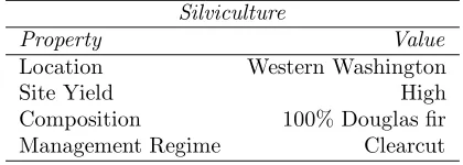
Table 1: Silvicultural and other site specific information. Silviculture

Property Value

Location Western Washington

Site Yield High

Composition 100% Douglas fir Management Regime Clearcut

Table 2: Forest owner specific parameters. Forest Owner Characteristics

Parameter Value

Replanting and Harvest Cost ($/MBF) 100 Annual Discount Rate (%/year) 5

Time Step Length (year) 1

years, with five years being the earliest possible harvest age producing commercially valuable timber. The stand was assumed to be 100% composed of Douglas fir, and the management regime to consist of clearcut harvests followed by immediate replanting. In all calculations, there was assumed to be one harvest opportunity ev-ery year between the stand ages of five and 100 years. Table 1 provides a summary of site specific properties.

Other parameters whose values had to be specified include the appropriate annual rate of discount and the magnitude of the harvest and replanting cost per MBF. Both of these parameters were assumed to vary across forest owners. In particular, the rate of discount was assumed to reflect the cost of capital to a given forest land owner rather than the risk-free rate. The values used in this article are given in Table 2.

In order to calculate the cashflows from Equations 12 and 13, it was necessary to specify the values of αand γ. αrepresents the percentage of sequestered carbon re-moved from the stand at harvest time, and its value was set to 60% by assumption. γ is a factor for converting atmospheric CO2 in metric tons to sequestered carbon in MBF of Douglas fir. Its value was determined from available data.

The prices of carbon and timber were modeled by the logarithmic mean-reverting stochastic process. The logarithmic mean-reverting process is conveniently de-scribed by the stochastic differential equation

dS_t=κ(μ−lnS_t)S_tdt+σ S_tdW_t, (20)

whereS_trepresents the price at timet,κstands for the rate of reversion to the long term trendμ, σstands for price volatility, anddW_tis an increment of the Wiener process.2

2_{From the perspective of microeconomic theory, the}

logarith-Table 3: Forest-owner-specific parameters. Carbon Parameters

Parameter Value

α(%) 60

γ (CO2ton/MBF) 3.6

Using Ito’s lemma, Equation 20 can be solved analyt-ically. The exact transitional density of lnS_t is normal and takes on the form

lnS_t∼N(Θ; Σ), (21)

where Θ = lnS0 + (1 −e−κt)(μ −σ2/2κ) and Σ = σ(1−e−2κt)_{/2κ. Because the distribution defined in} Model 21 is the exact solution of Equation 20, it can be used to simulate price paths ofS_twith an arbitrary step length, such as the one year length used in our simula-tions.

Table 4 contains the price model parameter values that were used during the simulations. These values were estimated from stumpage price data by linear re-gression. The only exception wasρ, which denotes the strength of the correlation between the elements of the bivariate Wiener process used in simulating the price paths of timber and carbon. The value ofρwas set to 10% by assumption, because the available time series did not overlap.

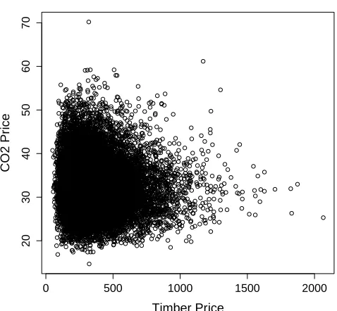
After the price model was chosen and calibrated, it was used to determine ¯S_t and ¯U_t, the sets of points on theS_tandU_t axis where the boundary curves of Equa-tions 14 and 15 would have to be calculated. The sim-plest way to determine ¯S_t and ¯U_tis to use Model 21 to simulate a large number of price paths over the entire length of the simulation horizon, in this case 100 years. Figure 2 contains a plot of the terminal values of 10,000 price paths from a typical simulation performed with the parameters set to values specified in Table 4.

The plot in Figure 2 shows that very few price paths terminated outside the rectangle whose upper right cor-ner was located at the $2000 dollar mark in the timber direction and the $100 mark in the CO2direction. These values were used to establish empirical upper limits of the domains of the optimal harvest boundaries of Equa-tions 14 and 15. The set ¯S_t was then formed from 40 values of S_tevenly spaced in the intervalS_t∈[0,2000]. Similarly, the set ¯U_t was formed from 20 values of U_t evenly spaced in the intervalU_t∈[0,100].

The product ¯S_t×U¯_t defines a grid of points in the S_t, U_t-plane where the estimates of the expected bare

Table 4: Parameter values for stochastic differential equations governing the behavior of timber and carbon prices.

Price Model Parameters

Parameter Timber Carbon

S0 400 ($/MBF) 25 ($/CO2ton) μ 6.0 (ln $/MBF) 3.5 (ln $/CO2ton)

κ(%/year) 0.35 4.0

σ(%/year) 0.4 0.5

ρ(%/year) 0.1

land value functions fi_{(S0, U0|·) would have to be}

cal-culated in order to evaluate Simulation 19.3

6

Simulation Results

The mean reversion property of the price model spec-ified by Equation 20, combined with the long time hori-zons characteristic of the optimal timber harvest prob-lem, suggests that current prices of timber and carbon should have only a small impact on expected bare land values,fi_{(S0, U0|·), for all but very low values of mean}

reversion rate κ. Instead, the long term price level μ should be the price model parameter most influential in determining bare land values.

In order to test this intuition, the expected bare land value of a single rotation (N = 1) was calculated for different pairs of starting timber and carbon prices on a 50×50 grid spanning the (0,2000)×(0,100) region of the S_t, U_t-plane. Four such simulations, each with re-initialized starting value of the random number gen-erator, were performed inR _?. In each of the four sim-ulations, a visual inspection of the results revealed no pattern, and the differences in the values offi(S0, U0|·) surface appeared to be caused by the random variation characteristic of Monte-Carlo results. A regression plane was fitted to each of the four datasets. All four planes were nearly flat over the region of interest, and there was no discernible pattern in the direction of the normal vec-tor: each of the planes was slightly tilted in a different direction.

These results indicate that, for mean reverting pro-cesses, the initial prices of timber and CO2 have only a minimal impact on expected bare land values with the simulation parameters as given above. This leaves the constant long-term price trendμ, price volatilityσ, rate of discount, and site productivity as the factors that

de-3_{For price models such as in Equation 20 that permit an} ana-lytical solution, these ranges can be determined exactly from the transitional density for a desired confidence level. However, this empirical procedure works well for more complex price models where the exact form of the transitional density is unavailable.

0 500 1000 1500 2000

20

30

40

50

60

70

Timber Price

CO2 Pr

ice

Figure 2: Estimate of the region containing the majority of end values of 50,000 timber and carbon price paths simulated over a period of 100 years.

termine bare land values. Because the expected bare land value surface is nearly flat over the relevant region of theS_t, U_t-plane, its estimatef1_(S

0, U0|·) need not be calculated in its entirety over a large grid of starting timber and carbon prices. It is sufficient to calculate

f1_(S

0, U0|·) at a single point (S0, U0) located, for ex-ample, near the center of the region of interest. This approach greatly reduces the amount of calculations re-quired to estimate f1(S0, U0|·) as well as the estimates of future rotation valuesfi(S0, U0|·) fori∈2, . . . , N.

Another potentially significant reduction of computa-tional effort may be realized by judiciously choosingN, the number of rotations. Performing several simulations for increasing values ofNcan help assess the rate of con-vergence in the number of rotations. The results of these simulations for parameter values of Tables 1 through 4 are illustrated in Figure 3.

1 2 3 4 5 6

2900

3000

3100

3200

Convergence in Number of Rotations

Number of Rotations

Expected Bare Land V

alue ($/acre)

Figure 3: Convergence is achieved after four rotations (i.e. N = 4). Each of the six box-plots indicating the combined value of future harvests was generated from nine sample runs.

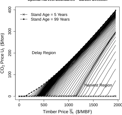
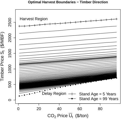
As discussed previously, the solution to the stochas-tic optimal harvest problem consists not only of the ex-pected bare land value but also of the optimal harvest boundary, which serves as a decision-making rule for the forest owner with regard to optimal harvest timing. The shape of the optimal harvest boundary curves for the stand used in this analysis is revealed by Figures 4 and 5. The boundary curves in Figure 4, specified by Equa-tion 14, were calculated for 40 evenly spaced values of the timber price ¯S_t∈[0,2000]. The boundary curves in Figure 5, specified by Equation 15, were calculated for 20 evenly spaced values of the CO2 price ¯Ut ∈[0,100].

All intermediate values were approximated by linear in-terpolation.

For a given stand age t, each of the optimal harvest boundaries depicted in Figure 4 separates the S_t, U_t -plane into harvest and delay regions. As described in the previous section, a point on a boundary curve is cal-culated by holding the selected timber price fixed at ¯S_t while searching for the corresponding carbon price U∗ that equalizes value of harvesting today with the ex-pected discounted value of harvesting harvesting later. The region below a given curve is the harvest region, because in this area timber prices are high relative to carbon prices. In the region above the curve is the delay

0 500 1000 1500 2000

0

100

200

300

400

Optimal Harvest Boundaries − Carbon Direction

TimberPriceS_t ($/MBF)

CO

2

Price

Ut

($/ton)

Delay Region

Harvest Region Stand Age = 5 Years

Stand Age = 99 Years

Figure 4: Eachgt_(S

t) curve initially runs along the

hor-izontal axis and then deviates upward. Note that the size of the delay region decreases with increasing stand age.

region, because the revenue from carbon sequestration is relatively high there. Note that as the stand age in-creases, the size of the harvest region increases at the expense of the delay region,i.e. a mature stand is more likely to get harvested.

The optimal harvest boundary curves depicted in Fig-ure 5 are obtained, for a given stand aget, by fixing the price of carbon at ¯U_t while searching for the price of timber S∗ that equalizes the value of harvesting imme-diately and the expected discounted value of harvest-ing later. As in the previous case, each of the bound-ary curves separates the price plane into harvest and delay regions. However, in Figure 5, the harvest re-gion is above each curve, because carbon prices are rel-atively low there and do not justify further harvest de-lay. Hence, the stand should be harvested immediately if timber prices are above the boundary. The delay region is located below the boundary curve where carbon prices are relatively high and timber prices relatively low, thus harvest should be delayed to maximize revenue from car-bon payments. As before, the area of the harvest region increases as the stand matures.

0 20 40 60 80

0

500

1000

1500

2000

2500

Optimal Harvest Boundaries − Timber Direction

CO₂PriceU_t ($/ton)

Timber

Price

St

($/MBF)

Delay Region Harvest Region

Stand Age = 5 Years Stand Age = 99 Years

Figure 5: Each ht_(U

t) curve separates the price plane

into delay and harvest regions for a given age of the standt. Note the decrease in the size of the delay region with increasing stand age.

constant and, hence, a fixed optimal rotation length can be determined. Such a strong result cannot be obtained when prices are stochastic. In order to maximize profit, forest owners must adjust harvest timings in response to price fluctuations. Figure 6 depicts the frequency distri-bution of recorded harvest ages for a sample simulation run and indicates that, given the above values of sim-ulation parameters, the mode harvest age is about 40 years. In order to reveal the full shape of the harvest time distribution, the minimal harvest age was set equal to two years, even though the commercial value of the stand at that age is minimal. The sudden increase in the number of harvests at the end of the simulation horizon is an artifice of the finite simulation horizon that would not be observed in reality.

7

Summary

This article presented a Monte-Carlo-based methodol-ogy for the solution of the multi-period optimal harvest problem with stochastic prices of timber and CO2. The solution algorithm extends the work of Ib´a˜nez and Zap-atero 2004 and provides a flexible alternative to the nu-merical methods based on finite difference schemes that have been previously employed in the literature.

For illustrative purposes, the methodology was

em-20 40 60 80 100

0

500

1000

1500

2000

2500

Harvest Age Frequency Distribution

Stand Age (Years)

Har

v

est Age Frequency

Figure 6: Frequency distribution of harvest timings for 50,000 simulated price paths with corresponding 50,000 antithetic paths. The typical harvest age for the stand used in the analysis is about 45 years.

ployed to calculate the expected bare land value for a Douglas fir stand that was assumed to be located on a high yield site in western Washington State. In addi-tion to calculating expected bare land values, the opti-mal harvest boundaries used for decision making with regard to harvest timing were also calculated for each age where harvesting the stand is possible. The results of expected bare land value calculations and the optimal harvest boundaries were then discussed. Additionally, a frequency distribution of optimal harvest ages was pre-sented and discussed.

8

Acknowledgements

The authors would like thank two anonymous review-ers for helpful comments on the manuscript. The au-thors are solely responsible for any remaining errors.

References

Brazee, R. J., and D. H. Newman, 1999. Observation on recent forest economics research on risk and uncer-tainty. Journal of Forest Economics 5(2):193–200.

Chladna, Z., 2007. Determination of optimal rotation period under stochastic wood and carbon prices. For-est Policy and Economics 9(8):1031–1045.

Dixit, A., and R. Pindyck, 1994. Investment under Un-certainty. Princeton University Press, Princeton, NJ.

Glasserman, P., 2004. Monte Carlo Methods in Financial Engineering. Springer-Verlag, New York.

Haight, R. G., 1993. The economics of Douglas-fir and red alder management with stochastic price trends. Canadian Journal of Forest Research 23:1695–1703.

Hull, C., John, 2003. Options, Futures, and Other Derivatives. Prentice Hall, Upper Saddle River, NJ.

Ib´a˜nez, A., and F. Zapatero, 2004. Monte Carlo valua-tion of American opvalua-tions through computavalua-tion of the optimal exercise frontier. Journal of Financial and Quantitative Analysis 39(2):253–275.

Insley, M., 2002. A real options approach to the valua-tion of a forestry investment. Journal of Environmen-tal Economics and Management 44:471–492.

Insley, M. C., and K. Rollins, 2005. On solving the multi-rotational timber harvesting problem with stochastic prices: A linear complementarity formulation. Ameri-can Journal of Agricultural Economics 87(3):735–755.

Kaya, J., and J. Buongiorno, 1987. Economic harvesting of uneven-aged northern hardwood stands under risk: A Markovian decision model. Forest Science 33:889– 907.

Lohmander, P., 1987. The economics of forest man-agement under risk. Report 79, Swedish University of Agricultural Sciences, Department of Forest Eco-nomics, Umea.

Morck, R., E. Schwartz, and D. Stangeland, 1989. The valuation of forestry resources under stochastic prices and inventories. The Journal of Financial and Quan-titative Analysis 24(4):473–487.

Newman, D. H., 1988. A discussion of the concept of the optimal forest rotation and a review of the recent liter-ature. General Technical Report SE-48, USDA Forest Service, Southeastern Forest Experiment Station.

Norstrom, C. J., 1975. A stochastic model for the growth period decision in forestry. The Swedish Journal of Economics 77(3):329–337.

Plantinga, A. J., 1998. The optimal timber rotation: An option value approach. Forest Science 44(2):192–202.