WOOD QUALITY ASSESSMENT OF TREE TRUNK FROM THE
TREE BRANCH SAMPLE AND AUXILIARY DATA BASED ON
NIR SPECTROSCOPY AND SILVISCAN
Chris J Cieszewski, Mike Strub, Finto Antony,
Pete Bettinger, Joseph Dahlen, Roger C Lowe
WSFNR, University of Georgia, Athens GA 30602 USA
Abstract. We estimated wood quality parameters for a specific tree trunk using samples of this tree’s
branch, and auxiliary samples from other similar species, based on analysis of wood density, modulus of elasticity (MOE), and microfibril angle (MFA), measured with the near-infrared spectroscopy (NIRS) and SilviScan processes. The measured materials included a branch sample from the subject tree, also known as the Smolensk birch, and stem analysis disk samples from silver birch (Betula pendula Roth) trees collected in central Poland. We analyzed and modeled the pith-to-bark and base-to-tip density changes in the silver birch samples, and using developed models estimated the subject tree trunk air-dry wood quality parameters and compared them with published yellow birch (Betula alleghaniensis) and silver birch tabular data. Then we compared the corresponding surrogated green wood parameters of the subject tree against the standard American utility wood pole parameters, and identified environmental adjustments necessary for a realistic and accurate representation of the final subject tree wood characteristics. The final conclusions from this study are that the subject tree dry wood parameters are not significantly different (in the statistical sense) from the well-documented yellow birch parameters, which were used as their surrogate, and even without the due reductions in parameters for excessive amount of whorls and branches, and for the height of the tree break (5 to 7 m above ground), the structural parameters of the subject tree green wood, as applicable to live tree and as surrogated by appropriate yellow birch parameters, are generally weaker than corresponding dry wood parameters for the standard American wood poles and weaker then the southern yellow pine parameters. The adjustments for the whorls and knots and height of the break may yield some additional 50% reduction in the estimates for the subject tree structural wood parameter values.
Keywords: Smolensk birch; Smolensk crash; silver Birch, Wood Quality; MOE; Wood Density; SilviScan; Green Wood; Log Grading; Knots in Lumber; Wood Engineering; Wood Pole Standards; Southern Pine.
1
Background
In the subsequent text we use the following abrivia-tions: NIRS – near-infrared spectroscopy; MFA – mi-crofibril angle; MOE – modulus of elasticity; MOR – modulus of rapture; MC – moisture content; CCD – charge-coupled device; CI – confidence interval; and SE – standard error.
Density, MFA and MOE are all important properties for assessing the suitability of wood for various struc-tural uses. Density is a ratio of oven-dried (i.e., 0% MC) wood weight to its volume under ambient con-ditions (Megraw, 1985). Density provides an estimate
of amount of cell wall material in a given volume of wood, and it is an important wood property, because it is strongly correlated with the structural strength of wood. MFA is the angle made by microfibrils in the S2 layer of the cell wall with the longitudinal axis of the cell (Megraw, 1985). MFA has a strong influence on stiff-ness, strength and dimensional stability of wood and is an important determinant of the quality of timber (Mac-Donald and Hubert, 2002). MOE describes the stiffness of a material and it is expressed as the ratio between stress and strain. The density, MFA, and MOE are im-portant characteristics when determining the structural quality of wood produced by a tree, and they are nec-Copyright©2013 Publisher of theMathematical and Computational Forestry & Natural-Resource Sciences
essary for all architectural and construction calculations of wood structure designs and for assessing mechanical behaviors underlying the destruction of all wood struc-tures (or trees) in response to external forces such as winds, snowfall, and collisions with other objects. Re-cently, state of the art technologies such as near infrared spectroscopy (NIRS) and the SilviScan process, which utilizes X-Ray diffraction, X-Ray absorption, and an image analysis system for fast and accurate measure-ments of wood quality parameters, have been used to measure a range of wood properties. These technolo-gies are being increasingly used as they provide a rapid, non-destructive measure of wood properties and are less dependent on sample preparation than other older tech-nologies (Evans and Ilic, 2001; Schimleck et al., 2002, 2005).
In this study we conducted comparative analysis of wood densities, MOE, and MFA, measured using NIR and SilviScan on wood samples from a branch of a spe-cific subject tree of interest, called hereafter “the sub-ject tree” and from auxiliary samples of stem analy-sis1 disks from silver birch trees collected in the re-gion of Minsk Mazowiecki in central Poland, called here-after silver birch. The subject tree is likely (Appendix B) a silver birch from Smolensk, Russia, that is also sometimes referred to as the “Smolensk birch”2 . Ac-cording to the report of Interstate Aviation Commit-tee (2011a,b) this tree is growing at the geographical coordinates of 54◦49.4940 north latitude and 32◦03.4220 east longitude, and was broken at an unknown and in-accurately reported height of about 5 to 8 m. For ex-ample, CINAA (2011); Interstate Aviation Committee (2011a,b) reported about 5 m height, but Polish Mili-tary Prosecutor Office reported 7.7 m at one time and 6.6 at another (e.g., www.wprost.pl). According to our measurements conducted in this study on ground pho-tography (Appendix A) the subject tree was likely bro-ken at about 6.5 m height; and therefore, we herein refer to this issue as 5 to 7 m height. We use a branch sam-ple from the lower part of this tree’s trunk to estimate the wood quality parameters for the tree trunk, and to compare them with the measurements of the silver birch stem analysis samples from Poland, and with tabular data for downy birch (Betula pubescensEhrh) and silver birches from Poland and Finland and for other American commercial birch tree species.
1Stem analysis is a sampling technique used for
reconstruct-ing past life timeseries of tree growth based on dissectreconstruct-ing trees (e.g., cutting sample disks from them or splitting them open) and measuring their rings insight tree bole.
2The Smolensk birch is the term used to describe the birch tree
that allegedly on April 10, 2010, near the Smolensk airport, broke off part of the left wing on the Polish Air Force One TU-154M plane causing it to crash with 96 fatal casualties including the President of Poland and 10 NATO generals.
The subject tree branch was harvested by a Polish journalist during his visit in Smolensk on April 13 and 14, 2010. The silver birch materials were contributed by a group of Polish scientists who collected a number of wood samples from stem analysis conducted in the area of Minsk Mazowiecki, in central Poland, which has similar climatic growth conditions to Smolensk, Russia. The subject tree branch analyzed in this study is the only known to date viable wood sample for this tree. Since the time of the incident, the broken tree has de-teriorated due to a destructive fungi infestation; and therefore, no viable wood samples can be reliably an-alyzed (Wilcox, 1978) from this tree break vicinity3. At the same time, the subject tree has recently become an object of many scientific inquiries (Binienda, 2011; Czachor, 2012; Interstate Aviation Committee, 2011a,b; Nowaczyk, 2012), and it is becoming an important issue that the relevant wood quality parameters be estimated for this tree. The parameters are needed for engineering calculations and computer simulation research investi-gating various aspects of the alleged collision of the Pol-ish Air Force One TU-154 plane with the subject tree. They are also needed for assessment of relevance of ear-lier similar research findings such as those in Murray (2007); Murray et al. (2005), who used previously esti-mated wood quality parameters of southern yellow pines for defining a Wood Material Model relevant to the dis-cussed simulations. Furthermore, the research interests in this area are extending to other studies of plane col-lisions with wooden objects (Reed et al., 1965), such as the American utility wood poles. Therefore, we have also included in our research the consideration for the wood quality parameters of the standard American util-ity wood poles discussed in Reed et al. (1965), which are made predominantly of the southern pines, and for the specific parameters of the southern yellow pines found in Murray (2007).
Since the starting point of this research originates with basic material, such as the wood samples, and any data used later in the analysis are in essence derived from the subsequently selected methods applied to the start-ing materials, we first describe the basic materials and then the methods along with the obtained from them data. Then in the Results and Discussion sections, we discuss the results of our analyses and findings and their associated implications and meaning. Finally, at the end of this article we offer a recapture of the main conclu-sions from this study and recommendations for further research.
3A number of scientists voiced this opinion, among others
Objectives of the Study
The primary objective of this study was to derive from our data analysis dependable theoretical estimates of wood quality parameters and their practically realistic variances for the subject tree and their likely dependence on height and radial location. We set out to determine if the wood quality parameters of the subject tree were significantly different from the wood quality parameters of our silver birch samples and other published birches. The most desirable outcome of this objective was to de-termine if the estimates wood quality parameters of the subject birch wood could be satisfactorily surrogated by wood quality parameters of any of the well-known and documented birch tree species. A positive outcome of such a match would enable further exploration of all other mechanical wood properties of the subject tree be-yond the data and analysis of our research.
The secondary objective of this study, based on a liter-ature review, was to compare the estimated wood quality parameters for the subject tree against the wood quality parameters of the standard American wood poles param-eters for consideration of Reed et al. (1965) studies, and against the wood quality parameters for southern yel-low pines used in Murray (2007); Murray et al. (2005) for considerations of described therein research. To this extent the goals of this objective were to:
1. assess the generally expected wood quality param-eters for utility poles; and
2. compare the above results against the determined wood quality properties for the green wood of the subject tree.
Finally, the third objective of this study was to iden-tify any significant environmental factors, such as knots and open growth conditions, which should be accounted for before considering the final wood quality parameter estimates for the subject tree in this study.
2
Materials
The materials for this research consisted of:
1. the branch sample of the subject tree, which we be-lieve is likely silver birch (Appendix B), harvested from the lower part of the tree trunk of this tree in Smolensk, Russia, at geographical coordinates of 54◦49.4940 north latitude and 32◦03.4220east longi-tude (Interstate Aviation Committee, 2011a,b), by Dr. Jan Gruszynski during his visit in Smolensk on April 13 and 14, 2010;
2. stem analysis disc samples from silver birch trees harvested in area of Minsk Mazowiecki in central Poland;
3. literature review of the wood quality parameters for different species and wood pole production stan-dards; and
4. photographs of the subject tree and derived from them measurements.
The primary wood quality measurements for this study were derived from the subject tree branch of 5 cm diameter and about 30 cm length that was cut from the subject tree. The branch sample was collected from the base of the tree on Apr. 13, 2010, and it was sub-sequently air-dried and stored in dry indoor conditions until June 2012 when we received it for analysis.
A number of silver birch trees were destructively sam-pled for stem analysis from natural stands. Disks 5 cm in thickness were sampled at different height levels (0, 5, 1.3, 1.5 m and every 1 m interval up to the tip of each tree) from the felled trees. One set of disks from a sin-gle tree and one piece of a stem chosen at random from a collection of trees was also selected for the described here analyses. All the samples were examined by wood quality experts for any anomalies, wood rot, insect or fungus damage, or any physical or chemical damages before they were accepted for further processing in the USDA Forest Service Wood Quality sample preparation shop. Any samples that might have had even just mi-nor fungal staining were trimmed of the stained surface, and cut using only their sound and undamaged parts of wood.
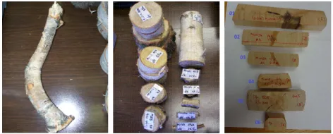
Figure 1: From left: picture of the subject tree branch sample; all sample disks; final samples cut to SilviScan specifications. The six samples selected for SilviScan analysis and subsequent calibration of local instrumen-tation. Birch wood samples 01-04 were cut from one Polish tree; 05–sample from 2nd Polish tree; 06–sample from the subject tree.
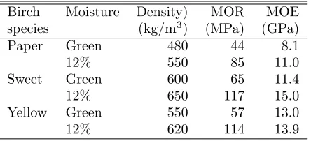
Table 1: Major Wood Quality Properties for birch com-mercial tree species.
Birch Moisture Density) MOR MOE species (kg/m3) (MPa) (GPa)
Paper Green 480 44 8.1
12% 550 85 11.0
Sweet Green 600 65 11.4
12% 650 117 15.0
Yellow Green 550 57 13.0
12% 620 114 13.9
subject tree and a Polish tree (Fig. 1). Subsequently selected six samples (four from one tree, one from other silver birch, and one from the subject tree) were sent to FP Innovations facilities in Vancouver, B.C., Canada, for the SilviScan analysis, while the other samples were provided to the wood quality laboratory at the Univer-sity of Georgia. Radial strips, 2 mm by 7 mm (respec-tively radial and tangential) and length depending on the disk radius were cut from 2 cm by 2 cm blocks and used for SilviScan analysis.
Various published materials for comparison of wood quality parameters between different species are avail-able in the literature for species of birch and for other species alike. Studies that have explored within tree variation of wood properties of birch are limited, but they are well documented, and there is a wealth of published information about the southern pine species, which is the primary species used for standard wood pole production. The published birch data used in this study come from the Wood Handbook published by the U.S. Department of Agriculture Forest Products Laboratory (2010). Examples of published data include the aver-age property values of wood from the most important commercial birch species as summarized in Table 1.
The wood pole standards have a long history in America as it began around 1915. The data on the properties and production standards of the wood poles are well summarized in Wolfe and Moody (1997) in addition to various source materials, such as AITC (1993); ANSI (1992, 1993, 1995, 1996); ASAE (1996); ASTM (1996a,b,c,d,e); AWPA (1997); Bodig and An-thony (1992); EPRI (1985, 1986); Kressbach et al. (1996); Micklewright (1992); REA (1982); Wood et al. (1960); Wood and Markwardt (1965). The American wood poles are produced according to ANSI standards and have to comply with required wood quality param-eters. As such they are relatively well predictable in terms of knowing their structural parameters and the type and quality of wood that they are made of.
From among many pictures of the subject tree available, two were taken for this study to com-pute the proportion of knots and whorls on the stem around the break point. The pictures were obtained from the Smolensk Conference website at www.Smolenskcrash.com photo galery. The selected pic-tures of the subject tree (Fig. 2) were originally taken on April 11thand 13th, 2010, by different photographers.
Figure 2: The subject tree break point. On the left pic-ture reproduced from Figure No. 27 published on page 84 of Interstate Aviation Committee (2011a,b) reports; and on the right picture taken by Dr. Jan Gruszynski on April 13th, 2010.
3
Methods and Data
3.1 The SilviScan analysis and measurements
The samples sent for SilviScan processing included the branch sample of the subject tree, four disks samples from a single tree of silver birch stem analysis, and one randomly chosen disk of silver birch from another tree. Wood properties of the radial strips, 2 mm by 7 mm, were measured using the SilviScan (Evans, 1999; Evans et al., 1995) in a controlled environment of 40% rela-tive humidity at temperature 20◦C, (20 ℃) which is equivalent to 7.7% MC (moisture content). Density was measured at an interval of 25 ηm using X-ray densito-metry based on Beer’s Law, stating that the intensity of an x-ray beam passing through a sample is inverse exponentially related to thickness, while attenuation is correlated with density:
I=I0e−αmDT (1) where:
I0 is the incident x-ray beam,
D is the density,
T is the thickness, and
αm is the mass absorption coefficient.
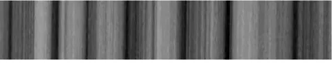
In SilviScan, an imaging camera with a 7 x 7ηm pixel CCD (charge-coupled device) scans the transmitted ra-diation through the wood sample and forms a gray-scale density image (Fig. 3), which is subsequently converted to nominal density using the attenuation coefficient es-timated from a cellulose acetate sheet obtained during calibration of the densitometer. The depth of scanning for the nominal density profile is 5 mm below the top surface of the sample, which is scaled subsequently to a true density profile based on calculated from volume (micrometry) and mass average density of the sample. This provides a dry basis density (8% moisture content), which can be converted as needed to basic or dry density using the swelling or shrinkage coefficient for any given species.
Figure 3: Example of magnified reconstituted density image.
MFA was measured using scanning X-ray diffractom-etry at an interval of 5 mm for these samples. SilviScan estimates MFA from the variance of the azimuthal (002) diffraction profile and the microfibril orientation distri-bution:
S2≈ µ
2 2 +σ
2 (2)
The (002) diffraction patterns are obtained from the planes whose normal is perpendicular to the microfib-ril axis. The variance (s2) of the azimuthal diffraction (002 - in Fig. 4) profile is related to the MFA (η) and the variance (σ2) of the microfibril orientation distribution (Evans, 1999; Evans et al., 1999).
In SilviScan, CCD x-ray detector detects and records the scattered beam of a focused x-ray beam (0.2 mm) going through the sample in the tangential direction. The recorded diffraction image is then mapped onto a spherical coordinate system with the azimuthal angles as horizontal and radial lines as vertical. Integrating over the radial limits of the 002 peaks extracts the intensity profile. The total variance of the profile (equation 2) includes the dispersion of microfibril orientation and the average MFA. MFA was acquired in integral mode (com-pared to point mode where MFA is acquired at a series of discrete points at any nominated segment) where MFA is averaged within the 5 mm segments along the sample.
Figure 4: Diffraction patterns obtained from SilviScan.
Spectral data (at 5 mm intervals) of samples of wood from pith to bark were used for the SilviScan analysis, and these were collected using the FOSS NIRSystem Inc. Model 5000 scanning spectrophotometer.
An estimate of MOE (MOEs are at the same resolu-tion as MFA) was obtained by combining the informa-tion of density and x-ray diffracinforma-tion (Icv) (Evans, 2006) as:
M OE=A(IcvD)B (3) where:
D is density from x-ray densitometry;
Icv is the coefficient of variation of the intensity of the x-ray diffraction profile, which includes the scattering from S2 layer and the background scattering from other cell wall constituents such as the S1 and S3 layers, parenchyma, and amorphous cellulose and lignin present in the fibre wall;
A and B are species independent statistical calibra-tion constants that relate to the sonic resonance method used for calibration (Evans, 2005).
Sonic testing usually provides higher values of MOE than static bending testing. The data provided by the SilviScan process were based on the reconstituted den-sity images of our samples (Fig. 5) and were provided in individual data files for each sample, with pith to bark profiles provided for each property evaluated by SilviScan (density, MFA, and MOE). Elastic proper-ties of wood vary in different directions, which can be calculated from elastic theory (Bodig and Goodman, 1973). Depending on the considered direction vary-ing from parallel to the fibers to perpendicular to the fiber the strength properties can be calculated from the Hankinson-type formula (?):
N = P Q
B)
E) C)
F) A)
D)
A)
B)
C)
D)
E)
F)
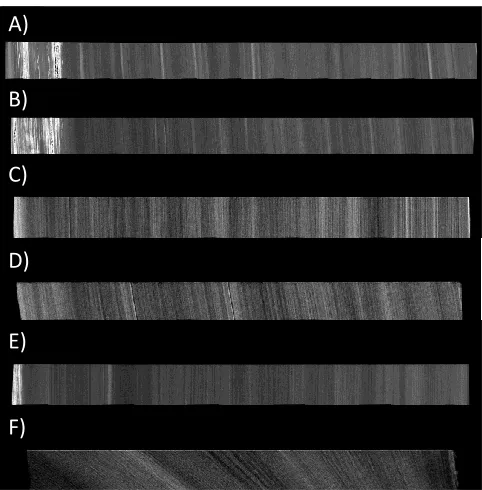
Figure 5: Reconstituted density images (reduced) of our samples provided by SilviScan (A-D four samples of one silver birch tree; E-randomly selected silver birch disk; F-the subject tree branch sample).
where:
N is strength at angleαfrom fiber direction,
Q is strength perpendicular to grain,
P is strength parallel to grain; and
n is an empirically determined constant.
Samples were held in a custom made holder with a 10 mm by 5 mm mask to ensure a constant area was analyzed (Schimleck et al., 2005). The spectra were col-lected at 2 nm intervals over the wavelength range of 1100–2500ηm. Wood property data collected by the Sil-viScan process and the corresponding spectral data from NIRs analysis were used to develop a calibration for den-sity, MFA and MOE using Partial Least Squares (PLS) regression with four cross validation segments (i.e., 25 percent of data was included in each validation segment using a systematic selection process). The wood prop-erty calibrations were developed using Unscrambler Soft-ware (Version 9.2) and second derivative spectra (left and right gaps of 4 nm were used for the conversion).
From the extra silver birch discs sampled from the tree, radial sections of 1.27 cm X 1.27 cm were cut from pith-to-bark, dried in an oven to a moisture content of 8% and glued into custom made core holders. Thin ra-dial strips of thickness approximately 1.6 mm were cut
from these sections using a twin-blade circular saw at the wood property lab of United States Department of Agri-culture, Forest Service, Athens, Georgia. NIR spectral data was collected from the radial face of these samples at 5 mm interval from pith-to-bark. The calibrations de-veloped above for density, MFA, and MOE were utilized to predict these properties of these extra samples at 5 mm interval.
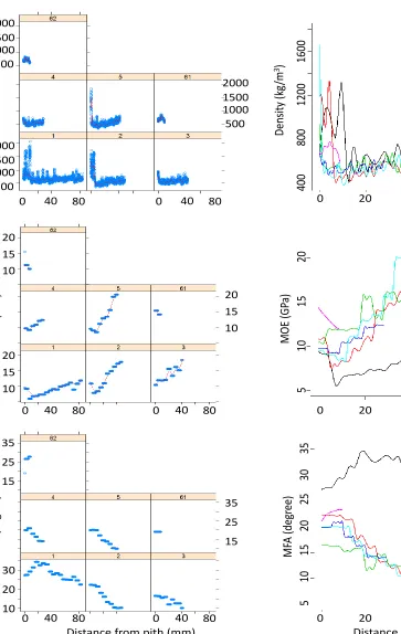
The obtained values were used to identify within tree variation of wood properties in birch and to compare the characteristics of branch wood with stem wood. Plots from the SilviScan measurements are illustrated on Fig-ures 6.
To investigate the within-tree, pith-to-bark, and stump-to-tip density patterns, we used models predict-ing property values from fitted spline regression models developed on the SilviScan data (Fig. 7). The spline regression models and their prediction graphs were sub-sequently used for visual analysis of the wood parameter characteristics and patterns under consideration.
3.2 The subject tree wood density and its vari-ation After applying the first disk of the subject tree branch to the SilviScan analysis and arriving at wood sample densities, MOE, and MFA for calibration of wood quality measurement in-house equipment (FOSS NIRSystems 5000 scanning spectrometer), we proceeded to determine the average 8% MC density that could be inferred from the branch sample. The average density of the subject tree was determined by two different means. First, the oven-dried samples from the segmented speci-men branch were measured for density (Tab. 2) by water displacement method and average density was calculated as an arithmetic mean of all the sub-samples exclud-ing the lowest and the highest measurements. However, since this method provides different means depending on at which points the sub-samples are selected, we used another method (Cieszewski, 2012) that was invariant under the choices of the sub-samples locations.
The second method was based on modeling the charac-teristic according to which:
1. the part of a branch adjacent to the main stem is likely to have higher densities than the trunk (Chmelar, 1992; Gryc et al., 2011; Gurau et al., 2008) and increasing towards the trunk, because of potential presence of compressed wood at the base of the branch and the transition of the branch wood towards the knot formation;
Den
si
ty
(kg
/m
3)
2000 1000 1500 500 2000 1000 1500 500Distance from pith (mm)
0 40 80
0 40 80
2000 1000 1500 500
MOE (
GP
a)
20 10 15Distance from pith (mm)
0 40 80
0 40 80 20 10 15 20 10 15
MF
A
(degr
ee)
35 15 25Distance from pith (mm)
0 40 80
0 40 80 30 10 20 35 15 25
Figure 6: Top: SilviScan density (25ηm) measurements at 8% MC determined in this study. Middle: SilviScan microfibril angle (5 mm) measurements at 8% MC de-termined in this study. Bottom: SilviScan modulus of elasticity (5 mm) measurements at 8% MC determined in this study.
Den
si
ty
(kg
/m
3)
Distance from pith (mm)
60 80
0 20 40
400
800
1200
1600
0.0 m 1.3 m 6.5 m 10.5 m Branch-Large Branch-Small
Distance from pith (mm)
60 80
0 20 40
5
10
15
20
0.0 m 1.3 m 6.5 m 10.5 m Branch-Large Branch-Small
MOE (
GP
a)
Distance from pith (mm)
60 80
0 20 40
5
10
15
20
25
30
35
0.0 m 1.3 m 6.5 m 10.5 m Branch-Large Branch-Small
MF
A
(degr
ee)
Table 2: Density measurements at different points of the branch sample at 8% MC.
Distance from the Density measurements branch base (cm) (kg/m3)
0 840.9 3 713.8 5 711.5 10 635.0 15 707.1 20 465.7 25 648.0
3. the part of a branch connecting the two above parts has the transitional value of wood density equal to the trunk density (Swenson and Enquist, 2008). Thus the most appropriate part of the branch matching the trunk density is likely around the curve convergence from the vertically asymptotic trend to the horizontally asymptotic trends of the curve (Fig. 8). The vertical asymptotic trend of the curve corresponds to the part of the branch near the trunk with a likely presence of compressed wood, where wood characteristics are chang-ing towards knot properties. The horizontal asymptote trend of the curve corresponds to the part of the branch away from the trunk with an increasing proportion of ju-venile wood (Kretschmann, 2008). Using this method, the selected value would be likely invariant under dif-ferent selections of the sub-samples, because the con-vergence point of the mathematical models fit into the result is unlikely to be much affected by different selec-tions of the sub-sample points used to define both of the asymptotic trends. Accordingly, we used an approach that seemed the most dependable and was based on fit-ting a mathematical model of the density convergence from the upper limit of the knot density to the lower limit of the juvenile part of the branch density.
After estimating the expected value of the trunk den-sity from the branch measurements the next step was to determine a reasonable variance around the estimate, in order to be able to determine realistically the sig-nificance of differences in estimates of mean parameters between the different sub-samples and between the sam-ples and the tabular data. The small sample size ob-tained from cutting the subject tree branch with large values of density at the base of the branch (with a max-imum of 841 kg/m3) and small values at the other end of the branch (466 kg/m3) would have an unrealistically high variance (SD = 114 kg/m3), which would make the comparisons of the mean density of the branch with the means of other samples meaningless. On the other
"Smolensk Birch" Sample Densities
600 650 700 750 800 850
0 20 40 60 80 100
Distance from the trunk (cm)
D e n s it y 1 2 % M C k g /m ^ 3 ) Measurements Model Extrapolation Convergence Tangent Line Branch Density Model
D e n si ty ( k g /m 3)
Distance from the trunk (cm) 60 80
0 20 40
6 0 0 6 5 0 7 0 0 7 5 0 8 0 0 8 5 0 Measurements Model Extrapolation Convergence Tangent Line Branch Density Model
100
Figure 8: Model of the relationship between density measurements of the Smolensk birch branch at 8% MC and the measurement distance from the branch base.
hand the altered data (with reduced weight of the out-lier) used for the model fitting had standard deviation (SD) of 77 kg/m3, which was still too high for a realistic comparison of different means. Calculating the standard deviation from the branch measurements with exclusion of the highest and lowest data points was leaving only five measurements points, of which two were at nearly the same point location of the branch, and it was likely underestimating the variance with SD=38 kg/m3 (even though the standard error of the regression was only 31.1 kg/m3) or more reasonably with excluding one of the close points, it wasSD= 40 kg/m3.
For the above reason we estimated a realistic variance from the larger sample of the SilviScan measurements, which were representative to both variations with height and with radial placement of the samples (Fig. 9). We investigated variances in the branch SilviScan measure-ments as well as the measuremeasure-ments of the other stem discs, so that the comparison of the means between the wood branch and the other birch samples may be more dependable. Table 3 contains partial summary statistics for the SilviScan data used in this task.
Dens
ity
(kg
/m
3
)
2000
1000
1500
500
Distance from pith (mm)
60
40
80
0
20
1
2
3
4
61
5
62
Figure 9: Estimation of realistic variation of the subject tree density at 8% MC.
exploratory analysis by fitting spline regression models to each individual height/sample measurements.
A flexible semiparametric regression method was used to explain the pith-to-bark nonlinear trend in wood properties; here air-dry density, Microfibril angle, and stiffness. Semiparametric regression can model nonlin-ear relationships without having any parametric restric-tion. The advantage is that these models can be for-mulated in a linear mixed model framework (Ngo and Wand, 2004), allowing the use of estimation and infer-ential tools available in mixed model methodology.
Let yijk represent the property observed at the kth distance from pith ofjthdisk ofithtree. A simple model form to explain the property with ring number is:
yijk= f(xijk) +εijk; whereεijk∼N 0, σε2
(5) where f is a smooth function describing the trend in a property with distance from pith. We utilized penal-ized smoothing splines, curves that are formed by splic-ing low-order polynomials at known knot locations, to model the change in wood properties with distance from pith. A truncated quadratic basis was used to model the functionf(xijk). The model (1) can be represented as:
yijk=β0+β1xijk+ +β2x2ijk+
PK
κ=1ur(xijk−κR) 2
++εijk (6) whereur∼N 0, σu2
. Here,κ1, . . . , κRare distinct knot locations within the range of xijk and (xijk−κR)+ is
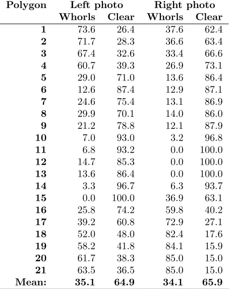
Table 3: Estimation of the relative knot areas in % on the stem of the subject tree using two photographs of the tree taken from slightly different angles. Polygons 6 and 15 represent the total areas of white and red polygons for right and left pictures respectively.
Polygon Left photo Right photo
Whorls Clear Whorls Clear
1 73.6 26.4 37.6 62.4
2 71.7 28.3 36.6 63.4
3 67.4 32.6 33.4 66.6
4 60.7 39.3 26.9 73.1
5 29.0 71.0 13.6 86.4
6 12.6 87.4 12.9 87.1
7 24.6 75.4 13.1 86.9
8 29.9 70.1 14.0 86.0
9 21.2 78.8 12.1 87.9
10 7.0 93.0 3.2 96.8
11 6.8 93.2 0.0 100.0
12 14.7 85.3 0.0 100.0
13 13.6 86.4 0.0 100.0
14 3.3 96.7 6.3 93.7
15 0.0 100.0 36.9 63.1
16 25.8 74.2 59.8 40.2
17 39.2 60.8 72.9 27.1
18 52.0 48.0 82.4 17.6
19 58.2 41.8 84.1 15.9
20 61.7 38.3 85.0 15.0
21 63.5 36.5 85.0 15.0
Mean: 35.1 64.9 34.1 65.9
the positive function where “+” sets it to zero for those values of xijk where xijk−κR is negative (here xijk <
κR). According to ?, a reasonable choice for selecting knots is that there should be 4-5 unique data points be-tween two knots, with 35 knots as the maximum number of allowable knots. They proposed a simple method for knot selection such that knotκr=
k+1 K+2
th
sample lo-cation of the unique x R ijk R’s, k = 1,. . . , R, where
K= max 5,min 1
4×number of uniquex
0
is, 35
. An estimate of [β, u] can be obtained by formu-lating the model (3) as a linear mixed model as Y = Xβ+ Zu +ε. The maximum likelihood estimate (MLE) of ˆβ and an empirical best linear unbiased pre-dictor for ˆucan be obtained by fitting the above model form in any standard mixed model software (e.g., lme in R). The smoothness of the curve is controlled by the parameterλ=σ2εσ2
u, which is calculated automatically using the restricted MLE’s ofσu2 andσ2ε.
branch sample is significantly different from that of sam-ples collected from the Smolensk birch tree. To test this hypothesis, we allowed the intercept to vary between the Smolensk birch branch sample and the samples collected from Poland. Then we used the significance of the dif-ferences between different intercept estimates to test the significance of the differences between different sampled trees.
3.4 Knots The whorl areas were segmented in Ar-cGIS, numbered and mark in red on Figure 2 (resulting in Fig. 10), which was used subsequently for calculating areas of all the polygons (see Appendix A for more de-tails). Based on the manual delineation of the knot and whorl areas on two pictures of the subject tree (Fig. 10) we have calculated the knot areas on each photo and listed the estimated data in Table 3.
Figure 10: The subject tree break point with manual whorls polygon delineation based on Figure 2. The red polygons are delimiting the whorls and the yellow poly-gons define the total area of the considered part of the stem.
4
Results and Discussion
Some of the pre-results of this study were described above along with the methods, and they were mainly pertinent to obtaining more detailed data for further analysis. In this section we discuss the final results and their interpretation. First we describe below the esti-mation results of the mean density for the subject tree branch and its variation in order to be able to find com-parable species that are well documented in the litera-ture. Next we discuss the analysis of the means and vari-ation of the silver birch and its wood parameter charac-teristics, so that the observed patterns can leverage the scant data from the subject tree of our investigation. The guiding principle for this stage of analysis is that if
the two birch samples, from the subject tree branch and from silver birch stem analysis, have similar wood prop-erty parameters then they likely will have also similar patterns of the properties of pith-to-bark changes and height changes of the samples. Then we find an appro-priate birch species that has been well documented in the literature and compare those to the standard utility poles characteristics, which are associated with the older studies of plane collisions with wood structures, such as the utility poles (Reed et al., 1965). In the end we present a discussion of other necessary adjustments for the most accurate assessment of the subject tree prop-erties along with a comparison of the subject tree wood properties with the expected parameters of the standard American utility wood poles.
4.1 The density of the subject tree branch wood and the SilviScan data analysis The two approaches of estimating the 8% MC average wood density near the base of the subject tree yielded similar results. The first approach, based on the oven-dried samples from the segmented specimen branch that were measured for density by water displacement method and averaged out as an arithmetic mean of all the samples, yielded values between 630 and 675 kg/m3 depending on whether the extreme values were used or not in the calculation and, whether only sub-samples from 5 to 25 cm were used in the calculations or whether all the sub-samples were used.
The second method, based on the mathematical mod-eling, yielded values from 625 to 665 kg/m3 depending on the inclusion of the lowest measurement (466 kg/m3) in the regression that had some characteristics of an out-lier. The sample density measurements were used to fit an asymptotic inverse half-saturation function that was then interpreted at the convergence tangential line that would most likely represent a value similar to the trunks density near the base of the tree where the branch was harvested. The final model was fitted to the data with recalculated value of the lowest measurement as an av-erage value of the previous, following, and its own value, which changed its value from 466 to 610 kg/m3. The final fit had 80% R2, and the model was estimating the conversion tangent point of the subject tree density near the base of the tree at 655 kg/m3, which was well within the range of expected values. The model describing the branch density changing with distance from the branch base was an inverse exponential function of the form:
D= 751.94r−0.0506 (7) where:
r is the distance in of the measurement from the base of the branch in mm.
The next step in the analysis of the average density for the subject tree data was an estimation of their variance for realistic significance tests of differences between the mean estimates for different samples and between the samples and the tabular data. The sub-sampling den-sity data of the sample branch had standard deviation of 114 kg/m3, which would make the mean of about 655 kg/m3 not significantly different from just about any tree species within a broad density range of 300 to 1,000 kg/m3 and would make any conclusions impossi-ble. Different options of estimating the variance were mentioned earlier, but the most robust option seemed to be using directly the SilviScan analysis data obtained for the branch. We obtained in total 719 measurements of density from two sub-samples of the branch. This was not good enough for estimation of the mean den-sity implied by the branch sample (each sub-sample of the branch had different mean density, and generally the density changes along the branch length), but it was sufficient for estimation of the variance around the es-timated mean density of the tree trunk at the height of the branch by the means of estimating the variance of the 719 measurements. The 719 density measure-ments ranged from 563 to 873 kg/m3 with a standard deviation of 54.25 kg/m3, which seemed very reasonable given all the other analysis and comparisons we con-ducted on all the SilviScan data in this study. Given the estimated mean density at the base of the subject tree of 655 kg/m3 derived earlier the 99.5% confidence interval would be approximately in the range of 546.5 – 763.5 kg/m3, which would easily contain just about any species of birch described in Table 1 and silver birch dis-cussed in (Her¨aj¨arvi, 2004b) with density of 566 kg/m3 at 12% MC. Note that the mean density for the whole bole (as applicable to the published tabular data) would have to be lower than 655 kg/m3; although, the paper birch with density of 550 kg/m3 at 12% MC (Tab. 1) and Finish silver birch described in (Her¨aj¨arvi, 2004b) with 566 kg/m3 at 12% MC would be only marginally suitable and possibly substantially underestimating the subject tree mean density. The silver birch and downy birch described in Her¨aj¨arvi (2004a) and Repola (2006) with mean densities of 538 and 467 kg/m3 at 8% MC wouldn’t even make this broad confidence interval. The unspecified birch species tested in Buchar et al. (2001) having density of 730 kg/m3at 7% MC would make this confidence interval with respect to wood density, but the MOE of this species of 16.1 GPa would be too high in comparison with the subject tree wood sample. How-ever, the silver birch populations in Lachowicz (2010b) could also be matched with the subject tree given its mean density of 681 kg/m3at 12% MC and an estimated
687 kg/m3at 8% MC, and even though the match is not as close as for the yellow birch it could be treated as up upper level bracketing of the possibilities for the subject tree wood properties.
Both the sweet birch (Betula lenta) and the yellow birch were suitable matches given densities of 650 and 620 kg/m3 respectively at 12% MC, and 655 and 628 kg/m3 at 8% MC; although, 650 kg/m3 (Tab. 1 and 5) for the mean density of the subject tree trunk would likely be an overestimation. Furthermore, since the sub-ject tree had the mean MOE of 12.61 GPa, the yellow birch with MOE 13.9 GPa at 12% MC and 14.3 at 8% MC (Tab. 1 and 5) was clearly a more appropriate fit to match the subject tree density and MOE than the sweet birch with MOE of 15 GPa at 12% MC and 15.5 GPa at 8% MC; and therefore, we have accepted yellow birch species as a surrogate for the subject tree. Fur-thermore, given the discussed above statistics and the data illustration on Figure 11 and 12, it is reasonable to assume that the silver birch from central Poland, as per Lachowicz (2010b), has also similar density character-istics to the subject tree and both of these two species can be assumed to represent similar densities and wood characteristics.
400 600 800 1000 1200 1400 1600 1800 2000
0 10 20 30 40 50
Dens
ity
(
kg
/m
3)
Radius (mm)
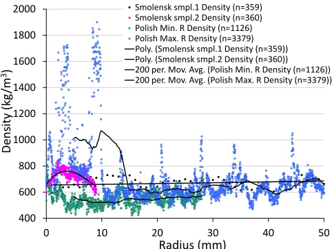
Smolensk smpl.1 Density (n=359) Smolensk smpl.2 Density (n=360) Polish Min. R Density (n=1126) Polish Max. R Density (n=3379) Poly. (Smolensk smpl.1 Density (n=359)) Poly. (Smolensk smpl.2 Density (n=360)) 200 per. Mov. Avg. (Polish Min. R Density (n=1126)) 200 per. Mov. Avg. (Polish Max. R Density (n=3379))
Figure 11: SilviScan data at 8% MC for the subject tree and for the highest and lowest density cookies sampled from the silver birch samples.
Den
si
ty
(kg
/m
3
)
Distance from pith (mm)
60
80
0
20
40
500
1000
1500
2000
Predicted – Tree Predicted – Branch Observed – Tree Observed – Branch
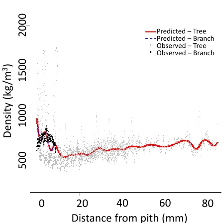
Figure 12: Predicted mean wood density curves at 8% MC for the silver birch and the subject tree within the large variability of the wood sample measurements.
ranging from about 700 kg/m3 down to 550 kg/m3 of wood 8% MC (Tab. 4) and even less in the higher parts of the tree not measured using SilviScan. The relation-ship between the mean density and the height of the tree was modeled using a part of averaged SilviScan data de-rived from a single tree (Fig. 13).
The mean density of the subject tree sample collected at the base of the tree was estimated as 655 kg/m3 and the weighted mean of density of the silver birch tree samples taken at the two lower relevant sections (Tab. 4) of the tree was 662 kg/m3. Given the ear-lier estimated variation of the subject tree measurements (SD = 54kg/m3) we conclude that both of the consid-ered species have similar means (Tab. 5) that are not sig-nificantly different from each other (in statistical sense at 95% confidence interval). Furthermore, since the sub-ject tree branch was harvested at a low height (where it could be easily reached by an individual) its measure-ments were likely to show much higher density than the one that may be expected at the break of the tree at about 5 to 7 m height. Given the evidence, that the subject tree wood density has similar spatial distribu-tion with height of the characteristics to the silver birch samples, and that the branch was harvested near the base of the tree, where the assumed wood density could have been estimated, depending on the adapted method, at values from 655 to 685 kg/m3, the model in Figure 13 estimates the mean dry wood density of the subject tree
Mean Density = 636.47 x Ht-0.0592
R2 = 0.9179
540
560
580
600
620
640
660
680
700
0
5
10
15
Me
an
D
e
n
si
ty
(
k
g
/m
3
)
Height of the Measurements (m)
Mean Density (SilviScan data)
Model of Mean Density = f(Ht)
Figure 13: Model of Mean Density at 8% MC as a func-tion of height based on SilviScan data of the silver birch.
at 5 m height to be on average about 580 kg/m3as per interpolation of the model in Figure 13 and the values indicated in Table 4. At 7 m height the average density is estimated to be about 568 kg/m3.
In addition to the general mean model we also develop a self-referencing model based on a dynamic equation to localize the predictions of the density changes with height to each of the observed actual measurements, so that we can illustrate the pattern of variation that is most likely associated with an error in the mean den-sity estimation. Assuming an anamorphic pattern of the modeled density characteristics we formulate a self-referencing algebraic difference approach based model describing the relationship of density (D) as a function of height (H) and a reference point of known density (D0) and height (H0) as:
D=D0
H
H0
−0.0592
Table 4: Part of the SilviScan measurements at 8% MCof discs obtained from different heights of one silver birch tree.
Data Model
Statistic Density MFA MOE Density MFA MOE
/ Variable (kg/m3) (Deg) (GPa) (Kg/m3) (Deg) (GPa)
No 1; Ht at base of about 0.3 m; n=3379
Mean 696.0 28.5 8.8 665.8 27.0 9.6
Min 471.0 22.4 5.9
Max 2036.0 34.3 11.8
Std 191.1 3.4 1.6
No 2; Ht=1.3 m; n=1926
Mean 603.7 15.5 12.7 562.8 12.9 14.5
Min 346.0 10.0 7.8
Max 1723.0 22.2 17.7
Std 219.9 4.8 3.5
No 3; Ht=6.5 m; n=1688
Mean 585.1 13.9 13.8 591.5 12.9 15.0
Min 438.0 9.9 14.0
Max 960.0 16.4 18.4
Std 69.8 2.1 2.3
No 4; Ht=13.0 m; n=1126
Mean 557.0 17.3 17.0 552.9 15.9 11.3
Min 423.0 14.0 9.2
Max 756.0 28.0 12.4
Std 52.4 2.6 1.1
for the subject tree, are illustrated on Figure 14, which demonstrates the range of possible densities of the sub-ject tree estimated as ranging from 557 kg/m3 to 594 kg/m3 at 5 m height and from 547 kg/m3to 582 kg/m3 at 7 m height.
Change of density from pith-to-bark is another com-mon characteristic of within-tree density variation. Her¨aj¨arvi (2004a) found a large radial variation (pith-to-bark, 40–80 kg/m3) and smaller vertical variation (20– 40 kg/m3) in density within Finnish birch trees. In an-other study, Her¨aj¨arvi (2004b) reported the static bend-ing properties of Finland grown downy and silver birch wood and reported an average MOE and MOR values of 14.5 GPa and 114 MPa for downy birch and 13.2 GPA and 104 MPa for silver birch. Her¨aj¨arvi (2004b) also found that both MOE and MOR increased from pith-to-bark and decreased from base to tip of the tree. In the samples analyzed in this study, we found that par-ticularly at the tree base and low heights, the density was extremely high near the pith, but then it was drop-ping dramatically a few to several cm from the pith and
subsequently was gently increasing towards the bark of the tree (see Fig. 12). At higher heights the extreme high density at the pith was not present and the density was simply increasing moderately from the pith towards the bark. The observed increases in density were vary-ing with height and they ranged from about 30 to as much as 150 kg/m3of the difference, which is a similar in magnitude to the decrease of the density with height of the SilviScan analyzed samples.
MFA showed a trend with low values near the cen-ter, increased afterwards until 10 mm from pith and decreased afterwards. MOE observed to be high near the pith, decreased immediately departing away from the pith and then increased as it is highly influenced by both density and MFA (SilviScan estimated MOE from density and MFA).
sam-Table 5: Mean values of densities at and Modulus of Elasticity for the samples of the subject tree, silver birch and the published values for American yellow birch.
Species / wood property Density (kg/m3) MOE (GPa)
Min. Mean Max. Min. Mean Max.
95% CI 95% CI 95% CI 95% CI
SilviScan data
Silver birch 8% H2O 630 12.1
The subject tree 8% H2O 547 655 764 8.3 12.6 16.9
Published tabular data
Yellow Birch 12% H2O 620 13.9
1Yellow Birch 8% H
2O 628 14.3
Sweet Birch 12% H2O 650 15.0
1Sweet Birch 8% H
2O 657 15.5
Silver Birch 12% H2O 681 14.0
2Silver Birch 8% H
2O 687 12.4 14.6 16.8
1For 8% MC estimation the green wood MC was assumed as 45% for sweet birch and at 47% for yellow birch. 2For 8% MC wood density adjustment of Lachowicz (2010b) data the green wood MC was assumed as 43% MC,
and the variation was estimated based on the smallest aggregation means reported in the source.
589
557
594
574
580
540
560
580
600
620
640
660
680
700
0 1 2 3 4 5 6 7 8 9 10 11
Den
si
ty
=
f(
Do
,Ho
,He
igh
t)
(kg
/m
3
)
Height of the Density (m)
Mean Density (SilviScan data)
Anamorphic Ht-Density Curves
Densities at Ht = 5 m
Model of Mean Density = f(Ht)
Figure 14: Anamorphic height-density curves estimated for the Smolensk birch data at 8% MC using SilviScan analysis.
ple is comparable in diameter with some of the disks collected from upper height levels of tree. The branch of the subject tree shows density that increases and then declines, MFA increases, and MOE decreases, which may be partially a function of the fact that the sub-sample of the branch was taken too close to the trunk with a small proportion of the compressed wood at the bottom of the branch sitting.
4.3 Results of the Semiparametric regression on the SilviScan data In the semiparametric regression approach to conduct the analysis on each property we used a nonparametric portion, which defines the nonlin-ear trend in pith-to-bark variation using a spline model. The parametric portion was used to test the difference between groups (2 groups, one encompassed the sam-ples from the subject tree branch and the other group was the samples from the silver birch stem analysis). The results of the semiparametric regression showed no significant differences between the densities of the two groups (Tab. 6). There were some differences between the MFA and stiffness of the two groups, which was ex-pected due to the fact that one group was obtained from a trunk of a tree and the other from a branch, which is expected to have more elastic wood properties.
Table 6: Results of the semiparametric regression on the SilviScan data from the subject tree branch sample and the silver birch samples. Measurements at 8% MC.
Statistics Parameters
Coef SE t-ratio p-value
Density (kg/m3)
Intercept -701.8 6602 -1063 9153
Slope 3817 8.588 04445 9645
Microfibril angle (Deg)
Intercept 15.8 37.79 4182 6758
Slope 1.175 3656 3.214 0013
Stiffness (GPa)
Intercept 5.498 41.58 1322 8948
Slope 3.052 154 19.82 0
above parameters for the subject tree were pertinent to air-dry wood (8% MC). These were the theoretical pa-rameters used for standardized description of wood qual-ity of the given sample and reliable comparisons made between the different samples. However, the air-dry wood parameters are not directly applicable (Gerhards, 1982; Mark et al., 1970; Wilson, 1932) to consideration of this tree strength during the time frame when the tree was alive; and therefore, all the relevant parameters de-scribing the subject tree wood properties need to be con-verted to the corresponding green wood values. It is very helpful for this purpose to use the subject tree surrogate of yellow birch, which is well documented in the litera-ture, and have all its parameters readily available from tabular data (Tab. 1). One could also consider using the silver birch surrogate parameters, but unfortunately they are not as well documented as the yellow birch pa-rameters especially with regards to the derivation of var-ious green wood parameters, which makes this choice impractical despite a fairly large body of literature on Polish silver birch wood properties (Lachowicz, 2008, 2010a,b, 2011a,b). Accordingly, we estimated the mean density of the subject tree green wood, when it was alive, as having theoretical values of 550 kg/m3, which needs to be adjusted using the applicable physical and environ-mental adjustments, and is subject to the discussed ear-lier variation and functional dependence on height and distance from the tree pith. We will also keep in mind that the choice of the Polish silver birch as the surro-gate species would yield approximately less than 10% inflation of the estimated density as compared to the choice of yellow birch as the surrogate species (i.e., 550
kg/m3/620 kg/m3×681 kg/m3= 604 kg/m3<1.1×550 kg/m3).
Estimation and comparison of the wood parameters for the standard American wood poles against the esti-mated parameters of the subject tree is important be-cause of the extensive study results derived in the testing of American airplanes in the past (Reed et al., 1965). The magnitude of the past studies and their extraor-dinary cost make any replication of similar studies im-possible and all of the past derived result very precious. For this reason, we must include the consideration of the American standard utility wood poles wood parameters in our study.
The American utility wood poles are produced accord-ing to ANSI standards and are well described in the lit-erature in all aspects of their specifications and dimen-sions (ANSI, 1992; Kressbach et al., 1996; REA, 1982; Wolfe and Moody, 1997), their construction and me-chanical properties (ASAE, 1996; ASTM, 1996b,e; Bodig and Anthony, 1992; EPRI, 1985, 1986), and their pro-duction standards and practices (ASTM, 1996c; AWPA, 1997). The majority of the standard utility wood poles are produced from the southern pines, which include the loblolly pine (Pinus taeda), longleaf pine (Pinus palus-tris), shortleaf pine (Pinus echinata), and slash pine (Pinus elliottii). These species also have very well doc-umented wood properties, which are listed herein along with the sweet and yellow birch wood properties in Ta-ble 7 (and Tab. 1). As evidenced in this taTa-ble the south-ern pine mean values for dry wood properties are gen-erally superior to those of green wood of either sweet or yellow birch (we couldn’t find any sources of silver birch green wood properties).
The differences in the wood parameters would be even greater if adjusted for a difference in height at the sce-nario at which the birch is considered at a height of 5 to 7 m while the pine in the tests described in (Reed et al., 1965) was considered at a height closer to the ground.
4.5 Physical and environmental adjustments for the subject tree wood properties In the earlier dis-cussed results of our analysis we demonstrated that the density of the subject tree sample was determined by various means as having the wood quality parameters similar to, or not significantly different from, the silver birch samples from central Poland, and the tabular val-ues of the Polish silver birch and the American yellow birch.
pro-T able 7: Strength prop erties of sw eet and y ello w birc h and sou thern pines and of the estimated southern pine w o o d p oles. Sp ecies name Moisture con ten t Densit y (kg/m 3) MOR: Mo du-lus of
rup- ture (MP
a) MOE: Mo du-lus of elas- ticit y (GP a) W ork to Max load (kJ/m 3)
Impact bend- ing (m) Compression parallel to
grai
n
(MP
a)
Compression perp
endicu-lar to grain (MP a)
Shear parallel to
grain (MP a) T ension p erp en-dicular to grain (MP a)
Side hard- ness (kN)
portions of early-wood and latewood are often consid-ered as qualifying parameters for the selection of wood samples for measurements of its density as a represen-tative parameter for a given species. Accordingly, the lumber selection often involves eliminating pieces that have exceptionally high proportions of early wood, which determines low wood density.
Presence of knots results in cross grain with steep slopes, which have the greatest effect on strength in ten-sion and perpendicular stresses; while in bending, the biggest effect may depend on whether or not a knot is on the tension or compression side of the stress (Coffey, 1962). The distortion of grain is greater around an in-tergrown knot than around an encased (or dead) knot of equivalent size; and therefore, the branches have a sig-nificant impact on trunk strength against perpendicular forces. The presence of a knot has a significant impact on most of the strength properties, and it depends on the proportion of the area of knots to the total area of the considered part of wood and the point of stress in the considered wood structure. The knots inside the considered piece of lumber are not very significant, but any whorls on a tree trunk cause significant weaken-ing of the trunk. Thus the most consideration needs to be given to the knots that are facing the outside lim-its of the structure, which in this case is the tree trunk. In construction practices knots are eliminated by pro-duction of glued-laminated structural members (AITC, 1993; ANSI, 1996) that are not continuous as in sawn structural lumber, but are knot free.
Based on the determination of the relative knot areas data derived from Figure 3 (Tab. 3) estimated knot areas to be about 35%, which implies a substantial reduction in the strength of the trunk as compared to its estimated originally theoretical value. This should be taken into account when considering setting the simulation param-eters at appropriate values, such as described in Mur-ray (2007) and evaluated in MurMur-ray et al. (2005). All the wood parameters in these documents are discussed under an assumption of a knot-free clear wood, which is much stronger than wood with knots. With 35% of large knot area in the outer layer of the tree trunk at the collision height the estimated value of green wood of the subject tree density may need 35% reduction in wood strength since large knots in the outer layer of the trunk are similar in impact to 35% of holes in the trunk. Thus, even the 520 kg/m3 of yellow pine density, which is assumed for calculations in Murray (2007) is a large overestimation of the subject tree density if used in the wood material model based simulations.
5
Summary
In this study we have analyzed the measurements of wood quality parameters for the subject tree, also known as the “Smolensk birch”, with respect to density, MOE, and MFA. The parameters were measured on various birch stem analysis samples from central Poland, and a branch sample from the subject tree. The objectives of the study included estimation of wood quality proper-ties for the subject tree and for the standard American wood poles and identifying necessary environmental ad-justments for the subject tree parameters.
The first objective dealt with estimating the density, MOE, and MFA, for the branch and stem analysis sam-ples, estimation of realistic means and variances, and comparison of their estimates between each of the tree species and against published tabular data. We used for the measurements of the samples state-of-the-art tech-nologies (NIRS and SilviScan), and in-house instrumen-tations for various wood testing and water displacement density measurements. The conclusion from this part of this research was that the subject tree wood mean pa-rameters at 8% MC were not significantly different from the well documented wood quality parameters published for the American yellow birch and Polish silver birch, and not significantly different from the mean param-eters of the analyzed in this study Polish silver birch samples. At the same time the published tabular data for the wood density of the American yellow birch was only about 10% lower than the published density data for the published Polish silver birch.
The second objective of this study was to conduct a review and comparisons of some of the most pertinent available literature on the subject of wood quality pa-rameters for the standard American utility wood poles. We discussed the standards of wood pole production, their expected wood quality parameters, and their phys-ical properties estimated as averages for the predomi-nant groups of species used in the wood pole produc-tion. These estimates are relevant to the comparison of the standard wood pole mechanical properties against the assessed mechanical properties of the subject tree. The conclusion from this research was that the estimated for the subject tree green-wood parameters were gener-ally weaker than the parameters of standard American wood poles, made from kiln-dry pressure-treated wood of predominantly southern pines, and they were weaker then the southern yellow pine parameters used in the LS-DYNA Wood Material Model (Murray, 2007; Murray et al., 2005).
the wood growth, structure and its mechanical proper-ties. Important elements affecting the wood mechani-cal properties are whorls, knots, and growth conditions, such as number of trees per unit area, reduction of wood density with height, inner rot, conks, and other defects that may be relevant to the analyzed object. In the case of the considered subject tree the most important adjust-ments identified included a correction for a large number of branches / knots and a correction for an open canopy growth conditions typically resulting in faster growth of lower density wood. The conclusion of this research was that due to excessive amounts of knots and whorls the subject tree realistic green-wood parameter values should be much weaker than their theoretical counter-parts estimated for this tree in the earlier part of this study. Accordingly, the adjusted wood quality parame-ter values for the subject tree green wood at the time of the April 10, 2010, incident should be much lower than the tabular parameters for the American yellow birch green wood, and consequently much lower than those of the kiln-dried standard American wood poles and the aforementioned southern yellow pines used in LS-DYNA Wood Material Model. While it is hard to estimate the exact number needed for the realistic adjustment, it is likely that a reasonable final adjustments of the subject tree parameters should likely be some 35% reduction of strength for the knots (Tab. 3) and about 15% to 17% reduction of the strength for the height of the break (Fig. 13) at about 5 to 7 m height.
The main highlights of the accomplishments of these studies are the following:
1. We estimated the theoretical values of the oven-dried wood quality parameters for both the silver birch samples (Tab. 4) and the subject tree branch (Tab. 5) using NIRS and SilviScan and mathemat-ical modeling of the density changes with height. We accepted 655 kg/m3 at 8% MC as the most re-alistic estimation of the subject tree wood density at the lower parts of the tree with a possible drop to about 580 kg/m3 to 569 kg/m3 at 8% MC at 5 to 7 m heights (Fig. 13 and 14). The corresponding with these estimates actual green wood densities of the subject tree would be respectively 581 kg/m3 at the lower part of the tree and 515 kg/m3to 505 kg/m3 at 5 to 7 m height of the subject tree. 2. Using existing ground photography pictures and
Ar-cGIS software we delimited the whorls and knot ar-eas near the tree break on the subject tree and com-puted the proportion of knots in this part of the tree (Tab. 3), which yield about 35% of external surface of the trunk near the break.
3. We compared the estimated parameters of silver birch with the subject tree parameters and tabu-lar data for Polish silver birch and American yellow birch, and concluded that they all were representing similar wood quality parameter values within about 10% spread of differences (Tab. 1, 4, 5).
4. Using literature review and published mechanical wood properties values we estimated expected wood quality parameters for the standard American wood poles produced predominantly from kiln-dried wood of southern pines (Tab. 7), and determined them to have stronger structural properties than the green wood of the subject tree (Tab. 7 and 3).
6
Conclusion and Recommendations
The main results of presented here research demon-strate that the subject tree dry wood mean parameters are not significantly different from the well-documented wood quality parameter information contained in the lit-erature of American yellow birch and the silver birch parameters, while the tree itself has unusually exces-sive amount of whorls and knots and the brake of the tree occurred at height of about 5 to 7 m, and both of these factors requires substantial additional strength pa-rameter reductions. Even without due reductions of the subject tree wood quality parameters for the excessive amount of whorls and knots, and for the height of the brake, its parameters for the green wood as surrogated by yellow birch green wood parameters, are generally weaker than the wood quality parameters for the stan-dard American wood poles and the southern yellow pine. With about 10% higher density the Polish silver birch green wood would possibly have similar or even pos-sibly marginally higher strength than the yellow pine, but the appropriate corrections of over 50% reduction, which we did not calculate in this study, would reduce significantly the wood quality parameters of the subject tree, which would make them much weaker than those of the standard American utility wood poles made from southern pines or the wood quality parameters used for southern yellow pines in the LS-DYNA Wood Material Model (Murray, 2007; Murray et al., 2005).
The main recommendations from this study for further research are that:
especially at higher heights (Swenson and Enquist, 2008);
2. the models developed here for height-density re-lationship and branch-trunk density rere-lationships are worth pursuing and perfecting with a stronger data, which we recommend to analyze using the self-referencing generalized algebraic differences ap-proach and fixed-effects fitting procedures;
3. the wood quality parameters estimated here for the subject tree have such a large margin of infe-riority in comparison with the standard American wood poles and southern yellow pine that it seems not worthwhile to do further research on improving these parameters; however, if such a research were desired and to be conducted we recommend one of the two, or both, approaches listed below to secure reasonable chances of success:
(a) a DNA analysis and typing may point in ex-isting databases to other species or even tree individuals that may have similar DNA typ-ing, which doesn’t guarantee the same wood properties, but which may allow for confirm-ing or lookconfirm-ing for the best surrogate trees for analysis; and/or,
(b) increment bores from the area of Smolensk of the same birch species could be collected from different heights and followed by a develop-ment of a polymorphic self-referencing height-density model, which could be used with a lower part (hopefully still healthy) of the sub-ject tree increment bore sample to predict the density at different heights near the subject tree break where the wood has deteriorated and where no reliable sample can be anymore collected.
Acknowledgements
This study was sponsored by the D.B. Warnell School of Forestry and Natural Resources, University of Geor-gia, Athens, GA, USA. Many thanks are due to the re-tired independent journalist Dr. Jan Gruszynski for se-curing the sample branch from the subject tree, and to Mrs. Ewa Skomorowska and prof. Piotr Witakowski for helping us to obtain this wood sample for our analysis. We are grateful to a number of Polish scientists who con-tributed to this study by providing the Polish silver birch samples and assisted us in the Polish literature search on silver birch wood quality parameters. Finally, we want to convey our gratitude to the three anonymous review-ers who provided many helpful comments on the earlier version of this manuscript and to Dr. Bob Megraw who
is one the top world experts in Wood Quality studies and who graciously agreed to be the journal guest editor for the peer-review of this manuscript.
References
AITC (American Institute of Timber Construction). 1993. Standard specification for glued laminated tim-ber of softwood species. AITC-117-93-Design. AITC, Englewood, CO.
ANSI (American National Standards Institute). 1992 Wood poles, specifications, and dimensions. ANSI 05.1. ANSI, New York.
ANSI. 1993. National electric safety code. ANSI C2. ANSI, New York.
ANSI. 1995. Solid sawn-wood cross arms and braces-specifications and dimensions. ANSI 05.3. ANSI. New York.
ANSI. 1996. Structural glued laminated timber for util-ity structures. ANSI 05.2. ANSI, New York.
ASAE (American Society of Agricultural Engineers). 1996. Design properties of round, sawn, and laminated preservative-treated construction poles. ASAE EP388, Agricultural Engineers Handbook.ASAE, St. Joseph, MI.
ASTM (American Society for Testing and Materi-als. 1996a. Standard methods for establishing de-sign stresses for round timber piles. Vol. 4.09, ASTM D2899. ASTM, West Conshohocken, PA.
ASTM. 1996b. Standard specification and methods for establishing recommended design stresses for round timber construction poles. Vol 4.09, ASTM D3200. ASTM, West Conshohocken, PA.
ASTM. 1996c. Standard practice for preservative treat-ment of utility poles by the thermal process. ASTM D4064. ASTM, West Conshohocken, PA.
ASTM. 1996d. Standard specifications for round tim-ber piles. Vol 4.09, ASTM D25-91. ASTM, West Con-shohocken, PA.
ASTM. 1996e. Standard test methods of static tests of wood poles. Vol 4.09, ASTM D1036-96. ASTM, West Conshohocken, PA.