Supervoxel-based segmentation of 3D imagery with optical flow integration for spatiotemporal processing

Xiaohui Huang, Chengliang Yang, Sanjay Ranka and Anand Rangarajan

Abstract

The past 20 years has seen a progressive evolution of computer vision algorithms for unsupervised 2D image segmentation. While earlier efforts relied on Markov random fields and efficient optimization (graph cuts, etc.), the next wave of methods beginning in the early part of this century were, in the main, stovepiped. Of these 2D segmentation efforts, one of the most popular and, indeed, one that comes close to being a state of the art method is the ultrametric contour map (UCM). The pipelined methodology consists of (i) computing local, oriented responses, (ii) graph creation, (iii) eigenvector computation (globalization), (iv) integration of local and global information, (v) contour extraction, and (vi) superpixel hierarchy construction. UCM performs well on a range of 2D tasks.

Consequently, it is somewhat surprising that no 3D version of UCM exists at the present time. To address that lack, we present a novel 3D supervoxel segmentation method, dubbed 3D UCM, which closely follows its 2D counterpart while adding 3D relevant features. The methodology, driven by supervoxel extraction, combines local and global gradient-based features together to first produce a low-level supervoxel graph. Subsequently, an agglomerative approach is used to group supervoxel structures into a segmentation hierarchy with explicitly imposed containment of lower-level supervoxels in higher-level supervoxels. Comparisons are conducted against state of the art 3D segmentation algorithms. The considered applications are 3D spatial and 2D spatiotemporal segmentation scenarios. For the latter comparisons, we present results of 3D UCM with and without optical flow video pre-processing. As expected, when motion correction beyond a certain range is required, we demonstrate that 3D UCM in conjunction with optical flow is a very useful addition to the pantheon of video segmentation methods.

Keywords: Supervoxels, Ultrametric contour map (UCM), Optical flow, Normalized cuts, Eigensystem

1 Introduction

The ready availability of 3D datasets and video has opened up the need for more 3D computational tools. Fur-ther, the big data era with ever improving computational resources allows us to envisage complex 3D processing methodologies with the anticipation of increased prac-ticality. The focus in the present work is on 3D seg-mentation. There is a clear and pressing need to extract coherent, volumetric, and spatiotemporal structures from high-dimensional datasets—specifically lightfields, RGBD videos and regular video data, particle-laden turbulent flow data comprising dust storms and snow avalanches,

*Correspondence:anandr@ufl.edu

Department of Computer and Information Science and Engineering, University of Florida, 32611-6120 Gainesville, FL, USA

and finally 3D medical images like MRIs. It is natural to represent coherent 3D structures in the form of locally homogeneous segments or irregularly shaped regions with the expectation that such structures correspond to objects of interest.

A particular focus of the present work is the parsing of volumetric and spatiotemporal datasets into supervox-els. While there exists previous work on this topic, the supervoxel literature is considerably sparser than the cor-responding superpixel literature. Supervoxels perform a similar function to superpixels: the codification of locally coherent, homogeneous regions. Superpixels and super-voxels have a conceptual connection to clustering since the latter is a popular way to extract coherent struc-tures from a set of patterns (using some imposed metric). However, the principal difference is that supervoxels can

benefit from the gridded structure of the data (which is not the case for general patterns). Consequently, success-ful supervoxel estimation techniques and the grouping algorithms at their center can be expected to leverage the “dense” nature of gridded 3D patterns.

The popular ultrametric contour map (UCM) frame-work [1] has established itself as the state of the art in 2D superpixel segmentation. However, a direct extension of this framework has not been seen in the case of 3D supervoxels. The current popular frameworks in 3D seg-mentation start by constructing regions based on some kind of agglomerative clustering (graph based or other-wise) of single pixel data. However, the 2D counterparts of these methods on which they are founded are not as accurate as UCM. This is because the UCM algorithm does not begin by grouping pixels into regions. Instead, it combines local feature information and global grouping in a two-step process which is responsible for its success. Therefore, it follows that a natural extension of this two-step process in the case of 3D should be a harbinger for success.

UCM derives its power from a combination of local and global cues which complement each other in order to detect highly accurate boundaries. However, all the other methods, with the exception of normalized cuts [2] (which directly obtains regions), are inherently local and do not incorporate global image information. In sharp contrast, UCM includes global image information by estimating eigenfunction scalar fields of graph Laplacians formed from local image features. Subsequently, the two pieces of information (local and global) are integrated to produce a good segmentation. Despite this inherent advantage, the high computational cost of UCM (mainly in its globaliza-tion step) is a bottleneck in the development of its 3D analog. Recent work in [3] has addressed this issue in 2D by providing an efficient GPU-based implementation but the huge number of voxels involved in the case of spa-tiotemporal volumes remains an issue. The work in [4] provides an efficient CPU-only implementation by lever-aging the structure of the underlying problem and provid-ing a reduced order normalized cuts approach to address the original computationally inefficient eigenvector prob-lem. Consequently, this opens up a plausible route to 3D as a reduced order approach effectively solving a closely related globalization problem but at a fraction of the cost. It should be noted that we do not expect the current rapid improvements in hardware and distributed process-ing to significantly improve the tractability of the origi-nal eigenvector problem in 3D, hence our foray into an approximate, reduced order, normalized cuts approach.

The main work of this paper has a tripartite structure. First, we design filters for 3D volumes (either space-time video or volumetric data) which provide local cues at multiple scales and at different orientations—akin

to the approach in 2D UCM. Second, we introduce a new method for graph affinity matrix construc-tion—henceforth called theoriented intervening contour cue—which extends the idea of the intervening contour cue in [5]. Third, we solve a reduced order eigenvec-tor problem by leveraging ideas from the approach in [4]. After this globalization step, the local and global fields are merged to obtain a new 3D scalar field. Sub-sequent application of a watershed transform on this 3D field yields supervoxel tessellations (represented as rela-tively uniform polyhedra that tessellate the region). The next step in this paper is to build a hierarchy of super-voxels. While 2D UCM merges regions based on their boundary strengths using an oriented watershed trans-form approach, we did not find this approach to work well in 3D. Instead, to obtain the supervoxel hierarchy, we follow the approach of [6] which performs a graph-based merging of regions using the method of internal variation [7].

The contributions of this work are summarized below:

• We present the first 3D UCM method for the segmentation problem. Our approach extends the popular and highly accurategPb -UCM framework (a technical term which will be elaborated below) to 3D resulting in a highly scalable framework based on reduced order normalized cuts. To the best of our knowledge, there does not exist a surface detection method in 3D which uses a graph Laplacian-based globalization approach for estimating supervoxels.

• It is a fully unsupervised method and it achieved state of the art performance on supervoxel benchmarks, especially having less fragmentation, better region quality, and better compactness. Further, our results indicate that owing to the deployment of a

high-quality boundary detector as the initial step, our method maintains a distinction between the

foreground and background regions by not causing unnecessary oversegmentation of the background at the lower levels of the hierarchy. This is especially clear in the video segmentation results presented in the paper.

• We expect applications of 3D UCM in a wide range of vision tasks, including video semantic

understanding and video object tracking and labeling in high-resolution medical imaging.

2 Related work

We first address previous work based on the normalized cuts framework. Subsequently, we attempt to summa-rize previous work on volumetric image segmentation with the caveat that this literature is almost impossible to summarize.

2.1 Normalized cuts andgPb-UCM

Normalized cuts [2] gained immense popularity in 2D image segmentation by treating the image as a graph and computing hard partitions. ThegPb-UCM framework [1] leveraged this approach in a soft manner to introduce globalization into their contour detection process. This led to a drastic reduction in the oversegmentation aris-ing out of gradual texture or brightness changes in the previous approaches. Being a computationally expensive method, the last decade saw the emergence of several techniques to speed up the underlying spectral decompo-sition process in [1]. These techniques range from various optimization techniques like multilevel solvers [8,9], to systems implementations exploiting GPU parallelism [3], and to approximate methods like reduced order normal-ized cuts [4,10].

2.2 3D volumetric image segmentation

Segmentation techniques applied to 3D volumetric images can be found in the literature of medical imaging (usually MRI) and 2D+time video sequence segmentation. In 3D medical image segmentation, unsupervised tech-niques like region growing [11] have been well studied. In [12], normalized cuts were applied to MRIs but gained little attention. Recent literature mostly focuses on super-vised techniques [13, 14]. In video segmentation, there are two streams of works. On the one hand, Galasso et al. and Khoreva et al.’s studies [15–18] are frameworks that rely on segmenting each frame into superpixels in the first place. Therefore, they are not applicable to gen-eral 3D volumes. On the other hand, a variety of other methods treat video sequences as spatiotemporal vol-umes and try to segment them into supervoxels. These methods are mostly extensions of popular 2D image seg-mentation approaches, including graph cuts [19,20], SLIC [21], mean shift [22], graph-based methods [6], and nor-malized cuts [9,23]. Besides these, temporal superpixels

while inter-supervoxel differences should be substantially larger; (iii) it is important that supervoxels have regular topologies; (iv) a hierarchy of supervoxels is favored as dif-ferent applications have difdif-ferent supervoxel granularity preferences.

2.3 Deep neural networks

over and beyond our current unsupervised learning UCM pipeline.

3 The supervoxel extraction framework

As mentioned in the Introduction, our work is a natu-ral extension of UCM, the state of the art 2D superpixel extraction approach. We now briefly describe the steps in 2D UCM since these are closely followed (for the most part) in our 3D effort.

UCM begins by introducing the Pb gradient-based detector which assigns a “probability” valuePb(x,y,θ)at every location (x,y) and orientation θ. This is obtained from an oriented gradient detectorG(x,y,θ)applied to an intensity image. A multiscale extensionmPb(x,y,θ)to the

Pbdetector is deployed by executing the gradient oper-ator at multiple scales followed by cue combination over color, texture, and brightness channels. Thus far, only local information (relative to scale) has been used. In the next globalization step, a weighted graph is constructed with graph edge weights being set proportional to the evidence for a strong contour connecting the nodes. This is per-formed for all pairs of pixels resulting in anN2×N2graph given N2 pixels. The top eigenvectors of the graph are extracted, placed in image coordinates followed by gradi-ent computation. This results in thesPb(x,y,θ)detector which carries global information as it is derived from eigenvector “images.” Finally, the globalized probability detector gPb(x,y,θ) is computed via a weighted linear combination of mPband sPb. While this completes the pipeline in terms of information accrued for segmenta-tion, UCM then proceeds to obtain a set of closed regions usinggPbas the input via the application of the oriented watershed transform (OWT). Watershed-based flood fill-ing is performed at the lowest level of a hierarchy leadfill-ing to an oversegmentation. A graph-based region merging algorithm (with nodes, edges, and weights corresponding to regions, separating arcs and measures of dissimilarity respectively) is deployed resulting in an entire hierarchy of contained segmentations (respecting an ultrametric). The UCM pipeline can be broadly divided into (i) thegPb

detector, (ii) the oriented watershed transform, and (iii) graph-based agglomeration.

The pipeline in our 3D UCM framework closely fol-lows that of 2DgPb-UCM with one major exception which will be clarified and elaborated upon below. The greater voxel cardinality forces us to revamp the globalization step above wherein a graph is constructed fromeverypair of voxels: if the volumetric dataset isN×N×N, the graph isN3×N3which is too large for eigenvector computa-tion. Therefore, computational considerations force us to adopt reduced order eigensystem solvers. A second excep-tion concerns the agglomeraexcep-tion step. 2D UCM merges regions together by only considering contour edge pix-els at the base level and not all pixpix-els. This approach

leads to the creation of fragmented surfaces in 3D. To overcome this problem, we perform graph-based agglom-eration using all voxels following recent work. With these changes to the pipeline, the 3D UCM framework is broadly subdivided into (i) local, volume gradient detec-tion, (ii) globalization using reduced order eigensolvers, and (iii) graph-based agglomeration to reflect the empha-sis on the changed subsystems. The upside is that 3D UCM becomes scalable to handle sizable datasets.

3.1 Local gradient feature extraction

The UCM framework begins with gradient-based edge detection to quantify the presence of boundaries. Most gradient-based edge detectors in 2D [43, 44] can be extended to 3D for this purpose. The 3D gradient operator used in this work is based on the mPb detector pro-posed in [1,45] which has been empirically shown to have superior performance in 2D.

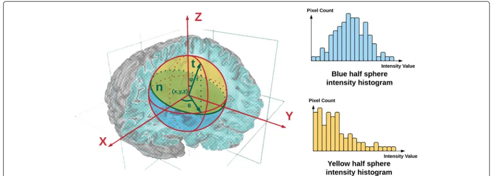
The building block of the 3DmPbgradient detector is an oriented gradient operatorG(x,y,z,θ,ϕ,r)described in detail in Fig.1. To be more specific, in a 3D volumetric or spatiotemporal intensity field, we place a sphere centered at each voxel to denote its neighborhood. An equato-rial plane specified by its normal vectort(θ,ϕ)splits the sphere into two half spheres. We compute the intensity histograms for both half spheres, denoted asgandh. Then we define the gradient magnitude in the directiont(θ,ϕ) as theχ2distance betweengandh:

χ2_(g,h)= 1

2

i

(g(i)−h(i))2

g(i)+h(i) . (1)

In order to capture gradient information at multiple scales, this gradient detector is executed for different radius values r of the neighborhood sphere. Gradients obtained from different scales are then linearly combined together using

Gs(x,y,z,θ,ϕ)≡

r

αrG(x,y,z,θ,ϕ,r) (2)

where αr weighs the gradient contribution at different

scales. For multi-channel 3D images like video sequences,

Gs(x,y,z,θ,ϕ)is separately calculated from each channel

and summed up using equal weights. Finally, the mea-sure of boundary strength at(x,y,z)is computed as the maximum response over all directionst(θ,ϕ):

mPb(x,y,z)≡max

θ,ϕ Gs(x,y,z,θ,ϕ). (3)

In our experiments,θandϕtake values in0,π₄,π₂,3₄π and−π₄, 0,π₄respectively and in one special case,ϕ =

π

2. Therefore, we compute local gradients in 13 different

directions. Neighborhood values of 2, 4, and 6 voxels were used forr. Equal weightsαr were used to combine

Fig. 1Theoriented gradient operator G(x,y,z,θ,ϕ,r): At location(x,y,z), the local neighborhood is defined by a sphere with radiusr. An equatorial planen(shaded green) along with its normal vectortsplits the sphere into two half spheres. The one abovenis shaded yellow and the one below is shaded blue. We histogram the intensity values of voxels that fall in the yellow and blue half spheres respectively. Finally, the local gradient magnitude is set to theχ2_{distance between the yellow and blue histograms in the directiontat scaler}

apply an isotropic Gaussian smoothing filter withσ = 3 voxels before any gradient operation.

3.2 Globalization using a reduced order eigensystem The globalization core ofgPb-UCM is driven by nonlinear dimensionality reduction (closely related to spectral clus-tering). The local cues obtained from the gradient feature detection phase are globalized (and therefore emphasize the most salient boundaries in the image) by computing generalized eigenvectors of a graph Laplacian (obtained from the normalized cuts principle) [2]. However, this approach depends on solving a sparse eigensystem at the scale of the number of pixels in the image. Thus, as the size of the image grows larger, the globalization step becomes the computational bottleneck of the entire pro-cess. This problem is even more severe in the 3D setting because the voxel cardinality far exceeds the pixel car-dinality of our 2D counterparts. An efficient approach was proposed in [4] to reduce the size of the eigensys-tem while maintaining the quality of the eigenvectors used in globalization. We generalize this method to 3D so that our approach becomes scalable to handle sizable datasets.

In the following, we describe the globalization steps: (i) graph construction and oriented intervening contour cue, (ii) reduced order normalized cuts and eigenvector computation, (iii) scale-space gradient computation on the eigenvector image, and (iv) the combination of local and global gradient information. For the most part, this pipeline mirrors the transition frommPbtogPbwith the crucial difference being the adoption of reduced order normalized cuts.

3.2.1 Graph construction and the oriented intervening contour cue

In 2D, the normalized cuts approach begins with sparse graph construction obtained by connecting pixels that are spatially close to each other.gPb-UCM [1] specifies a sparse symmetric affinity matrix W using the interven-ing contour cue [5] which is the maximal value ofmPb

along a line connecting the two pixels i,jat the ends of relationWij. However, this approach does not utilize all of

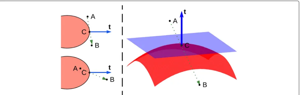
the useful information obtained from the previous gradi-ent feature detection step. Figure2describes a potential problem and our resolution. To improve the accuracy of the affinity matrix, we take the direction vector of the maximum gradient magnitude into consideration when calculating the pixel-wise affinity value. This new variant is termed the oriented intervening contour cue. For any spatially close voxelsiandj, we useij¯ to denote the line segment connectingiandj.dis defined as the unit direc-tion vector ofij¯. AssumePis a set of voxels that lie close toij¯. For anyp∈ P,nis the unit direction vector associ-ated with itsmPbvalue. We define the affinity valueWij

betweeniandjas follows:

Wij=exp

−max

p∈P{mPb(p)|d,n|}/ρ

(4)

where ·,· is the inner product operator of the vector space andρis a scaling constant. In our experiments, the setPcontains the voxels that are at most 1 voxel away from

¯

Fig. 2Left: Suppose we want to calculate the affinity value between voxelsAandB.Cis the voxel with maximalmPbvalue that lies on the line segmentAB¯. In the upper-left case,AandBbelong to one region. In the lower-left case,AandBare in two different regions. But the intervening contour cue of UCM [1] gives the same affinity value in both cases, which is not very satisfactory. Obviously it would be better if we consider the directiontofC’smPb.Right: In ouroriented intervening contour cueapproach, when calculating affinity values, we always take the product ofmPb(C)

with the absolute value of the inner productt,n, wherenis the unit direction vector of line segmentAB¯. IfAandBare on different sides of a boundary surface,|t,n|will be large, leading to small affinity value and vice versa

3.2.2 Reduced order normalized cuts and eigenvector computation

At this point, standard 2DgPb-UCM solves for the gener-alized eigenvectors of the sparse eigensystem

(D−W)v=λDv (5)

where D is a diagonal matrix defined by Dii = jWij.

However, this eigenvector problem is computationally very intensive. It becomes the bottleneck, both in time and memory efficiency, of the normalized cuts-based segmen-tation algorithms. To overcome this problem, an efficient and highly parallel GPU implementation was provided in [3]. However, this approach requires us to use GPU-based hardware and software suites—an unnecessary restric-tion at this stage of development. A clever alternative in [4, 10] builds the graph on superpixels instead of pix-els to reduce the size of the eigensystem. We chose to generalize Taylor’s [4] approach to 3D as (i) the super-pixel solution is more scalable than the GPU solution in terms of memory requirements, (ii) specialized GPU co-processors are not commonly available in many com-puting platforms like smart phones and wearable devices, and (iii) the approach in [10] is specifically designed for superpixels in each frame in video segmentation, thus not easily generalizable. Finally, the approach in [4] constructs a reduced order normalized cuts system which is easier to solve. We denotemas the number of supervoxels andnas the number of voxels. The reduced order eigensystem is denoted by

LT(D−W)L

x=λLTDLx (6) whereL ∈ Rm×n_{,x ∈ R}m_{andLx= v. The purpose ofL}

is to assign each pixel to a superpixel/supervoxel. In our

approach, the supervoxels are generated by a watershed transform on themPbimage obtained from the volumet-ric gradient feature detection step. Obviously, the number of supervoxels m is much smaller than the number of voxelsnin the 3D volumetric/spatio-temporal image. In practice, there are usually two to three orders reduction in the size of the eigensystem (from millions of voxels to few thousands of supervoxels). Therefore, it is much more efficient to solve Eq. (6) than Eq. (5).

3.2.3 Scale space gradient computation on the eigenvector image

We solve for the generalized eigenvectors{ x0,x1,. . .,xn}

of the system in (6) corresponding to the smallest eigen-valuesλ₀,λ₁,. . .,λ_n. As stated in [4],λi in (5) will be

equal toλ_iandLxiwill matchvimodulo an irrelevant scale

factor, whereviare the eigenvectors of the original

eigen-system (5). Similar to the 2D scenario [1], eigenvectorsvi

carry surface information. Figure3shows several example eigenvectors obtained from two types of 3D volumet-ric datasets. In both cases, the eigenvectors distinguish salient aspects of the original image. Based on this obser-vation, we apply the gradient operatormPbdefined in (3) to the eigenvector images. The outcome of this procedure is denoted assPbbecause it represents thespectral com-ponent of the boundary detector, following the convention established in [1]:

sPb(x,y,z)=

K

i=1

1 √

λi

mPbvi(x,y,z). (7)

Fig. 3Upper left: One slice of a brain MRI from the IBSR dataset [61].Lower left: One frame of a video sequence from the BuffaloXiph dataset [58].

Right: The corresponding slices/frames of the first 4 eigenvectors

weighting by 1/√λi is inspired by the mass-spring

sys-tem in mechanics [1,46]. In our experiments, we use 16 eigenvectors, i.e.,K =16.

3.2.4 The combination of local and global gradient information

The last step is to combine local cuesmPband global cues

sPb.mPbtries to capture local variations whilesPbaims to obtain salient boundary surfaces. By linearly combining them together, we get aglobalizedboundary detectorgPb:

gPb(x,y,z)=ωmPb(x,y,z)+(1−ω)sPb(x,y,z). (8)

In practice, we use equal weights formPbandsPb. After obtaining thegPbvalues, we apply a post-processing step of non-maximum suppression [43] to get thinned bound-ary surfaces when the resulting edges frommPbare too thick. Figure4shows some examples ofmPb,sPbandgPb.

3.3 Supervoxel agglomeration

At this point, 2DgPb-UCM proceeds with the oriented watershed transform (OWT) [1,47,48] to create a hierar-chical segmentation of the image resulting in the ultramet-ric contour map. However, we find that the same strategy does not work well in 3D. The reasons are twofold. First, because of the presence of irregular topologies, it is more difficult to approximate boundary surfaces with square or triangular meshes in 3D than to approximate bound-ary curves with line segments in 2D. Second, following OWT, during superpixel merging, only the information of the pixels on boundaries are used during greedy boundary removal. This is not a robust design especially when we take into account the fragmentation of boundary surfaces in 3D.

For the above reasons, we turn to the popular graph-based image and video segmentation methods [6, 7] to create the segmentation hierarchy. We first apply a water-shed transform to thegPbfield obtained from the previous step to get an oversegmentation. Next we iteratively merge

the adjacent segments beginning with this oversegmenta-tion. The output of this procedure is a segmentation hier-archy represented by a tree-structure whose lower-level segments are always contained in higher-level segments. As in [6], the merge rules run on a graph. The nodes of the graph are regions and the edges represent region to region relations. First, for any two adjacent regionsRiand

Rj, we assign an edgeeij to connect them on the graph.

The weight ofeijis set to theχ2 distance between (Lab

space) intensity value histograms ofRiandRjwith 20 bins

used. Also, for any regionR, a quantity named the relaxed internal variation RInt(R)is defined as follows:

RInt(R)≡Int(R)+ τ

|R| (9)

where Int(R) is defined as the maximum edge weight of its minimum spanning tree (MST). For the lowest-level regions, i.e., the regions of oversegmentation obtained from the watershed transform, Int(R)is set to 0.|R|is the voxel cardinality of regionR.τ is a parameter which trig-gers the merging process and controls the granularity of the regions. In each iteration of merging, all the edges are traversed in ascending order. For any edgeeij, we merge

incident regionsRi andRjif the weight ofeij is less than

the minimum of the relaxed internal variation of the two regions. Thus the merging condition is written as

weight(eij) <min{RInt(Ri), RInt(Rj)}. (10)

In practice, we increase the granularity parameterτ by a factor of 1.1 in each iteration. This agglomeration pro-cess iteratively progresses until no edge meets the merging criterion. The advantage of graph-based methods is that they make use of the information in all voxels in the merged regions. Furthermore, as shown in the experi-ments below, we see that it overcomes the weakness of fragmented supervoxels of previous graph-based meth-ods. This is because traditional graph-based methods are built on voxel-level graphs.

Finally, we obtain a supervoxel hierarchy represented by a bottom-up tree structure. This is the final output of the 3D UCM algorithm. The granularity of the segmentation is a user-driven choice guided by the application.

4 Integration with optical flow

Integration of 3D UCM with optical flow is quite nat-ural in the spatiotemporal setting. We would like to establish spatiotemporal coherence and stability of struc-tures across time and one way to achieve this is via the application of optical flow. Estimation of optical flow across multiple frames is a difficult problem: motion mod-els and optimization strategies are required to resolve the ambiguities and discontinuities prevalent. However, when multiple frames are simultaneously considered, we are afforded with the possibility of coupling supervoxel

estimation with multiframe optical flow. While this is straightforward to visualize in video segmentation, we argue that the registration of multiple frames across time can be of benefit in far-flung applications such as par-ticle flows in computational fluid dynamics and change detection in remote sensing.

Our work is an extension of 3D UCM supervoxel seg-mentation to the spatiotemporal case. The pipeline in the 3D UCM framework is to sequentially perform gradient feature extraction, globalization, and supervoxel agglom-eration on 3D volumetric images. In the spatiotemporal case, we precede 3D UCM by first bringing the mul-tiple frames into register using optical flow. This inte-gration is dubbed 3D OF UCM to denote the use of optical flow.

4.1 Optical flow computation

Optical flow has a complex relationship to the actual 3D motion field since it represents apparent motion caused by intensity change [49, 50]. Optical flow has been a central topic in computer vision since the 1980s and has considerably matured since then [51]. The basic approach consists of estimating a vector field (velocity vectors at each grid point) which is subsequently related to object motion.

In general, optical flow can be divided into two types, sparse optical flow and dense optical flow [51,52]. Briefly, the sparse optical flow method only computes flow vec-tors at some “interesting” pixels in the image, while the dense optical flow method estimates the flow field at every pixel and is more accurate [53,54]. We use dense optical flow here since we wish to integrate with scene segmentation.

4.2 Supervoxel segmentation

In recent work on video segmentation problems, motion estimation has emerged as a key ingredient for state of the art approaches [7,55,56] for both deep learning methods and typical methods. We introduced optical flow esti-mation to the pipeline of 3D OF UCM. On top of 3D UCM, we first compute optical flow and then consider to employ it as the source of an additional cue to guide the segmentation.

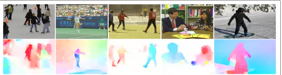
Fig. 5Examples of optical flow images.Top: RGB images.Bottom: corresponding motion magnitude estimates

Since our input data has additional optical flow infor-mation (a motion channel), we usually achieve better segmentation results especially for some small regions. As optical flow provides complementary information to RGB images, 3D OF UCM improves the overall performance. Datasets, evaluation metrics, and comparison results are presented in Section5.

5 Evaluation

We perform quantitative and qualitative comparisons between 3D UCM, 3D OF UCM, and state of the art supervoxel methods on different types of 3D volumetric and spatiotemporal datasets.

5.1 Experimental setup

5.1.1 Datasets

We use three video datasets for quantitative and qual-itative comparisons. The most typical use cases of 3D segmentation are medical images like MRIs and video sequences. We use the publicly available Internet Brain Segmentation Repository (IBSR) [61] for our medical imaging application. It contains 18 volumetric brain MRIs with their white matter, gray matter, and cerebro-spinal fluid labeled by human experts. These represent cortical and subcortical structures of interest in neuroanatomy.

The second dataset is BuffaloXiph [58]. It is a subset of the well-known xiph.org videos, and the 8 video sequences in the dataset have 69–85 frames with dense seman-tic pixel labels. The third dataset is the DAVIS dataset (Densely Annotated VIdeo Segmentation) [31], a bench-mark dataset designed for the task of video object segmen-tation. DAVIS contains 55 high-quality and full HD video sequences and densely annotated, pixel-accurate ground truth masks, spanning multiple occurrences of common video object segmentation challenges such as occlusions, motion blur, and appearance changes. For quantitative comparisons, we use the BuffaloXiph dataset and carry out experiments with a thorough quantitative analysis on a well-accepted benchmark, LIBSVX [28].

5.1.2 Methods

A comprehensive comparison of current supervoxel and video segmentation methods is available in [27,28]. Build-ing on their approach, in our experiments, we compare 3D UCM and 3D OF UCM to two state of the art super-voxel methods: (i) hierarchical graph based (GBH) [6] and (ii) segmentation by weighted aggregation (SWA) [8, 9, 62]. GBH is the standard graph-based method for video segmentation and SWA is a multilevel normalized cuts solver that also generates a hierarchy of segmentations. Some quantitative superpixel evaluation metrics have been recently used [63] for frame-based 2D images. For 3D spacetime validation, a comprehensive comparison of current supervoxel and video segmentation methods is available in [27,28].

5.2 Qualitative comparisons

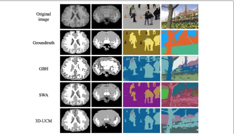
We present some example segmentation results for three datasets: IBSR, BuffaloXiph, and DAVIS. To compare GBH, SWA, and 3D UCM, we present some slices from both the IBSR and BuffaloXiph datasets in Fig.6. It shows that, through different levels, there are significant differ-ences in the segmentation results of all three methods. However, it is difficult to say which method is the best compared with the ground truth. It should be noted that GBH has a fragmentation problem in the IBSR and Buf-faloXiph datasets. On the other hand, SWA has a clean segmentation in IBSR but suffers from fragmentation in video sequences. In contrast, 3D UCM has the most regular segmentation.

Fig. 6The level of the segmentation hierarchy is chosen to be similar to the ground truth granularity.Left: IBSR dataset results. The white, gray and dark gray regions are white matter, gray matter and cerebro-spinal fluid (CSF) respectively.Right: BuffaloXiph dataset results

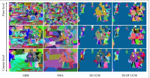
SWA both have a fragmentation problem in the Buf-faloXiph datasets through different levels. In contrast, 3D UCM has the most regular segmentation and 3D OF UCM has the finest segmentation even in small detailed regions. In general, 3D UCM generates meaningful and compact supervoxels at all levels of the hierarchy while

GBH and SWA have a fragmentation problem at the lower levels. To demonstrate the improved supervoxel agglomeration of 3D OF UCM compared to 3D UCM, we examine Fig.9which shows the original images, opti-cal flow images, segmentation from 3D UCM, and 3D OF UCM. The optical flow images generated prior to

Fig. 8The hierarchy of segmentations for the BuffaloXiph dataset.Left: GBH.Middle Left: SWA.Middle Right: 3D UCM.Right: 3D OF UCM

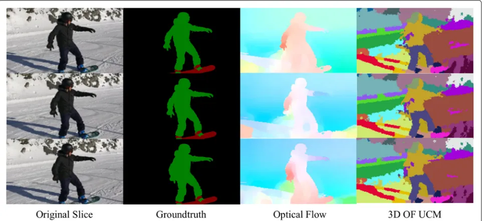
segmentation extract the boundaries of different objects and improve the supervoxel segmentation. For instance, the two legs of the person in the center of the image in Fig. 9 are grouped as the same supervoxel object by 3D OF UCM but segmented as different objects by 3D UCM. Also for the snowboard frames, 3D OF UCM gener-ates finer supervoxels for both the moving object and the background.

And in the DAVIS dataset, we selected some examples of optical flow and segmentation results of 3D OF UCM in Fig.10. It shows that 3D OF UCM generates fine super-voxels and avoids unnecessary oversegmentation of the

background for the moving object because of information from the optical flow motion channel. The result can be regarded as early video processing and be employed to other vision tasks, e.g., semantic segmentation and object segmentation. To sum up, 3D UCM leverages the strength of a high-quality boundary detector and, based on that, 3D OF UCM leverages additional flow field infor-mation to perform better. Hence, from qualitative com-parisons on two benchmark datasets, it suffices to say that 3D OF UCM generates more meaningful and com-pact supervoxels at all levels of the hierarchy than three other methods.

Fig. 10Optical flow estimation and supervoxel segmentation for multiple temporal frames on DAVIS dataset

5.3 Quantitative measures

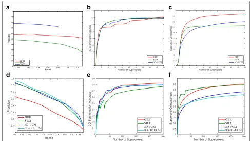
As both the IBSR and BuffaloXiph datasets are densely labeled, we are able to compare the supervoxel meth-ods on a variety of characteristic measures. Besides, we re-examined our 3D OF UCM experiments to quantify improvement by using optical flow as a complementary cue. In the previous experiment integrating optical flow with 3D UCM, we only compute optical flow for the first 15 frames and added flow vectors to the original RGB channels. In the next experiment, we process optical flow estimation for the complete video in the BuffaloX-iph dataset, and the results show more improvements. We posit the improvements mostly benefit from consistency of motion flow in video. For performance comparisons between 3D OF UCM and 3D UCM, the main improve-ments are demonstrated on quantitative measures. From the figures of quantitative measures, we notice that, except at very small granularity, 3D OF UCM perform better than 3D UCM on boundary quality, region quality, and supervoxel compactness.

5.3.1 Boundary quality

The precision-recall curve is the most recommended measure and has found widespread use in comparing image segmentation methods [1,45]. This was introduced into the world of video segmentation in [16]. We use it as the boundary quality measure in our benchmarks. It measures how well the machine generated segments stick to ground truth boundaries. More importantly, it shows the tradeoff between the positive predictive value (preci-sion) and true positive rate (recall). For a set of machine

generated boundary pixelsSband human labeled

bound-ary pixelsGb, precision and recall are defined as follows:

precision≡ |Sb∩Gb| |Sb|

, recall≡ |Sb∩Gb| |Gb|

. (11)

We show the precision-recall curves on IBSR and Buf-faloXiph datasets in Fig. 11a, d respectively. 3D UCM performs the best on IBSR and is the second best on Buf-faloXiph while 3D OF UCM perform the best. GBH does not perform well on BuffaloXiph while SWA is worse on IBSR. One limitation of 3D OF UCM and 3D UCM is that there is an upper limit of its boundary recall because it is based on supervoxels. GBH and SWA can have arbitrar-ily fine segmentations. Thus they can achieve a recall rate arbitrarily close to 1, although the precision is usually low in these situations. Since our 3D OF UCM adds a motion channel to 3D UCM, its boundary quality is better than 3D UCM.

5.3.2 Region quality

Measures based on overlaps of regions such as Dice’s coefficients are widely used in evaluating region cover-ing performances of voxelwise segmentation approaches [64,65]. We use the 3D segmentation accuracy introduced in [27, 28] to measure the average fraction of ground truth segments that is correctly covered by the machine-generated supervoxels. Given thatGv = {g1,g2,. . .,gm}

super-d

e

f

Fig. 11Quantitative measures.aIBSR, boundary.bIBSR, region.cIBSR, compactness.dBuffaloXiph, boundary.eBuffaloXiph, region.fBuffaloXiph, compactness

voxels generated by the algorithms, andV represents the whole volume, the 3D segmentation accuracy is defined as

3D segmentation accuracy≡ 1 m

m

i=1

n

j=1|sj∩gi| ×1(|sj∩gi| ≥ |sj∩gi|)

|gi|

(12)

whereg_i=V\gi. We plot the 3D segmentation accuracy

against the number of supervoxels in Fig.11b,e. GBH and SWA again perform differently in IBSR and BuffaloXiph datasets. But 3D UCM consistently performs well and 3D OF UCM shows the best performance on the BuffaloXiph dataset, especially when the number of supervoxels is low.

5.3.3 Supervoxel compactness

Compact supervoxels of regular shapes are always favored because they benefit further higher level tasks in com-puter vision. The compactness of superpixels generated by a variety of image segmentation algorithms in 2D was investigated in [66]. It uses a measure inspired by the isoperimetric quotient to measure compactness. We use another quantity defined in a similar manner to specific surface area in material science and biology. In essence, specific surface area and isoperimetric quotient both try to quantify the total surface area per unit mass or volume. Formally, given thatSv = {s1,s2,. . .,sn}are supervoxels

generated by algorithms, the specific surface area used to

measure supervoxel compactness is defined as

specific surface area= 1

n

n

i=1

Surface(si)

Volume(si)

(13)

where Surface() and Volume() count voxels on the surfaces and inside the supervoxels respectively. Lower values of specific surface area imply more compact supervoxels. The compactness comparisons on IBSR and BuffaloXiph are shown in Fig. 11c, f. We see that 3D UCM always generates the most compact supervoxels except at small supervoxel granularities on IBSR. GBH does not perform well in this measure because of its fragmentation problem, which is consistent with our qualitative observations.

6 Discussion

In this paper, we presented the 3D UCM supervoxel framework, an extension of the most successful 2D image segmentation technique,gPb-UCM, to 3D. Experimental results show that our approach outperforms the current state of the art in most benchmark measures on two dif-ferent types of 3D volumetric datasets. When combined with optical flow, 3D OF UCM performs very well on spatiotemporal datasets. The principal difference between 3D UCM and its 2D counterpart is a reduced order normalized cuts technique to overcome a computational bottleneck of the traditionalgPb-UCM framework when directly extended to 3D. This immediately allows our method to scale up to larger datasets. When we jointly consider supervoxel quality and computational efficiency, we believe that 3D UCM can become the standard bearer for massive 3D volumetric datasets. We expect applica-tions of 3D UCM in a wide range of vision tasks, including video semantic understanding, video object tracking and labeling in high-resolution medical imaging, etc.

Considering recent advances in deep learning-based methods on vision tasks, we investigated state of the art video segmentation methods using deep neural networks and also performed additional experiments on introduc-ing transfer learnintroduc-ing to the 3D UCM framework. For the BuffaloXiph dataset, we extracted its low-level features (first 1–4 layers from VGG-19 [41]) from the state of the art neural network, added to its original RBG chan-nels, and used the new data as input to our 3D UCM framework. The results did not show much improve-ment. In general, the transfer learning-based 3D UCM has very similar performance as 3D UCM. In some cases, the transfer learning-based 3D UCM has lower segmen-tation accuracy than 3D UCM since the CNN provided additional features are effectively noise w.r.t. supervoxel extraction. For this reason, we did not include this method in the paper. And this remained the case even after we did extra experiments with manually selected features. We posit that it is hard to get hierarchical segmentation from end-to-end deep learning networks because of the lack of multilevel dense annotation. We also did experiments similar to the pipeline of [67] using 3D UCM for video object segmentation on the Densely Annotated VIdeo Segmentation (DAVIS) dataset. Using supervoxels gener-ated by our proposed work, with optical flow and saliency map, our video object segmentation results demonstrate its effectiveness and top rank performance in comparison with other state of the art unsupervised methods.

Since this is a new and fresh approach to 3D seg-mentation, 3D UCM still has several limitations from our perspective. First, because it is a general purpose technique, the parameters of 3D UCM have not been tuned using supervised learning for specific applications. In immediate future work, we plan to follow the metric

learning framework as in [1] to deliver higher perfor-mance. Second, since it is derived from the modular framework ofgPb-UCM, 3D UCM has numerous alterna-tive algorithmic paths that can be considered. In image and video segmentation, a better boundary detector was proposed in [18], with different graph structures deployed in [17,68,69] followed by graph partitioning alternatives in [70, 71]. A careful study of these alternative options may result in improved versions of 3D UCM. A GPU implementation will almost certainly permit us to replace the reduced order normalized cuts eigensystem with the original eigensystem leading to better accuracy. Finally, 3D UCM at the moment does not incorporate prior knowledge for segmentation [72,73]. As transfer learning methods develop in 3D leading to the publication of use-ful 3D filters, these can be readily incorporated into the local feature extraction step of 3D UCM. These avenues represent relatively straightforward extension paths going forward.

Abbreviations

3D OF UCM: three dimensional optical flow UCM; CNNs: Convolutional neural networks; DAVIS: Densely annotated video segmentation; GBH: Hierarchical graph based;gPb-UCM: Globalized probability map UCM; IBSR: Internet brain segmentation repository; SWA: Segmentation by weighted aggregation; UCM: Ultrametric contour map

Acknowledgements

We acknowledge Manu Sethi for assisting us with the optical flow integration. This work is partially supported by NSF IIS 1743050 to A.R. and S.R.

Funding

Directorate for Computer and Information Science and Engineering (1743050).

Availability of data and materials IBSR:https://www.nitrc.org/projects/ibsr/

BuffaloXiph:https://www.cse.buffalo.edu/~jcorso/r/labelprop.html DAVIS:http://davischallenge.org/

Authors’ contributions

XH is the main driver of the optical flow integration. CY is the main driver of the 3D UCM implementation. SR made significant contributions in the reduced order normalized cut subsystem and provided overall leadership. AR made contributions to optical flow integration and provided overall leadership. All authors read and approved the final manuscript.

Competing interests

The authors declare that they have no competing interests.

Publisher’s Note

Springer Nature remains neutral with regard to jurisdictional claims in published maps and institutional affiliations.

Received: 23 June 2017 Accepted: 27 May 2018

References

1. Arbelaez P, Maire M, Fowlkes C, Malik J (2011) Contour detection and hierarchical image segmentation. IEEE Trans Pattern Anal Mach Intell 33(5):898–916.https://doi.org/10.1109/TPAMI.2010.161

2. Shi J, Malik J (2000) Normalized cuts and image segmentation. IEEE Trans Pattern Anal Mach Intell 22(8):888–905.https://doi.org/10.1109/34.868688 3. Catanzaro B, Su BY, Sundaram N, Lee Y, Murphy M, Keutzer K (2009)

7. Felzenszwalb PF, Huttenlocher DP (2004) Efficient graph-based image segmentation. Int J Comput Vis 59(2):167–181.https://doi.org/10.1023/B: VISI.0000022288.19776.77

8. Sharon E, Brandt A, Basri R (2000) Fast multiscale image segmentation. In: IEEE Conference on Computer Vision and Pattern Recognition. IEEE Vol. 1. pp 70–77.https://doi.org/10.1109/CVPR.2000.855801 9. Sharon E, Galun M, Sharon D, Basri R, Brandt A (2006) Hierarchy and

adaptivity in segmenting visual scenes. Nature 442:810–813.https://doi. org/10.1038/nature04977

10. Galasso F, Keuper M, Brox T, Schiele B (2014) Spectral graph reduction for efficient image and streaming video segmentation. In: IEEE Conference on Computer Vision and Pattern Recognition. pp 49–56.https://doi.org/ 10.1109/CVPR.2014.14

11. Pohle R, Toennies KD (2001) Segmentation of medical images using adaptive region growing. In: Proceedings of SPIE 4322, Medical Imaging 2001: Image Processing. pp 1337–1347.https://doi.org/10.1117/12. 431013

12. Carballido-Gamio J, Belongie SJ, Majumdar S (2004) Normalized cuts in 3-D for spinal MRI segmentation. IEEE Trans Med Imaging 23(1):36–44. https://doi.org/10.1109/TMI.2003.819929

13. Fischl B, Salat DH, Busa E, Albert M, Dieterich M, Haselgrove C,

van der Kouwe A, Killiany R, Kennedy D, Klaveness S, Montillo A, Makris N, Rosen B, Dale AM (2002) Whole brain segmentation: Automated labeling of neuroanatomical structures in the human brain. Neuron 33(3):341–355. https://doi.org/10.1016/S0896-6273(02)00569-X

14. Deng Y, Rangarajan A, Vemuri BC (2016) Supervised learning for brain MR segmentation via fusion of partially labeled multiple atlases. In: IEEE International Symposium on Biomedical Imaging.https://doi.org/10. 1109/ISBI.2016.7493347

15. Galasso F, Cipolla R, Schiele B (2012) Video segmentation with superpixels. In: Asian Conference on Computer Vision, Lecture Notes in Computer Science. Springer, Berlin Vol. 7724. pp 760–774.https://doi.org/ 10.1007/978-3-642-37331-2_57

16. Galasso F, Nagaraja NS, Cárdenas TJ, Brox T, Schiele B (2013) A unified video segmentation benchmark: Annotation, metrics and analysis. In: IEEE International Conference on Computer Vision. pp 3527–3534.https://doi. org/10.1109/ICCV.2013.438

17. Khoreva A, Galasso F, Hein M, Schiele B (2015) Classifier based graph construction for video segmentation. In: IEEE Conference on Computer Vision and Pattern Recognition. IEEE. pp 951–960.https://doi.org/10. 1109/CVPR.2015.7298697

18. Khoreva A, Benenson R, Galasso F, Hein M, Schiele B (2016) Improved image boundaries for better video segmentation. In: European Conference on Computer Vision Workshops. Lecture Notes in Computer Science. vol. 9915. Springer, Cham. pp 773–788.https://doi.org/10.1007/ 978-3-319-49409-8_64

19. Boykov YY, Veksler O, Zabih R (2001) Fast approximate energy minimization via graph cuts. IEEE Trans Pattern Anal Mach Intell 23(11):1222–1239.https://doi.org/10.1109/34.969114

20. Boykov YY, Jolly MP (2001) Interactive graph cuts for optimal boundary & region segmentation of objects in N-D images. In: IEEE International Conference on Computer Vision. IEEE Vol. 1. pp 105–112.https://doi.org/ 10.1109/ICCV.2001.937505

21. Achanta R, Shaji A, Smith K, Lucchi A, Fua P, Süsstrunk S (2012) SLIC superpixels compared to state-of-the-art superpixel methods. IEEE Trans Pattern Anal Mach Intell 34(11):2274–2282.https://doi.org/10.1109/ TPAMI.2012.120

22. Paris S, Durand F (2007) A topological approach to hierarchical segmentation using mean shift. In: IEEE Conference on Computer Vision

for temporal window objectness. In: IEEE International Conference on Computer Vision. pp 377–384.https://doi.org/10.1109/ICCV.2013.54 27. Xu C, Corso JJ (2012) Evaluation of super-voxel methods for early video

processing. In: IEEE Conference on Computer Vision and Pattern Recognition. IEEE. pp 1202–1209.https://doi.org/10.1109/CVPR.2012. 6247802

28. Xu C, Corso JJ (2016) LIBSVX: A supervoxel library and benchmark for early video processing. Int J Comput Vis 119(3):272–290.https://doi.org/10. 1007/s11263-016-0906-5

29. Cordts M,Omran M,Ramos S,Rehfeld T,Enzweiler M, Benenson R, Franke U, Roth S, Schiele B (2016) The cityscapes dataset for semantic urban scene understanding. In: IEEE Conference on Computer Vision and Pattern Recognition. pp 3213–3223.https://doi.org/10.1109/CVPR.2016.350 30. Fragkiadaki K, Arbeláez P, Felsen P, Malik J (2015) Learning to segment

moving objects in videos. In: IEEE Conference on Computer Vision and Pattern Recognition. pp 4083–4090.https://doi.org/10.1109/CVPR.2015. 7299035

31. Perazzi F, Pont-Tuset J, McWilliams B, Gool LV, Gross M, Sorkine-Hornung A (2016) A benchmark dataset and evaluation methodology for video object segmentation. In: IEEE Conference on Computer Vision and Pattern Recognition. pp 724–732.https://doi.org/10.1109/CVPR.2016.85 32. Fragkiadaki K, Zhang G, Shi J (2012) Video segmentation by tracing

discontinuities in a trajectory embedding. In: IEEE Conference on Computer Vision and Pattern Recognition. IEEE. pp 1846–1853.https:// doi.org/10.1109/CVPR.2012.6247883

33. Koh YJ, Kim CS (2017) Primary object segmentation in videos based on region augmentation and reduction. In: IEEE Conference on Computer Vision and Pattern Recognition. pp 7417–7425.https://doi.org/10.1109/ CVPR.2017.784

34. Tokmakov P, Alahari K, Schmid C (2017) Learning video object segmentation with visual memory. In: IEEE International Conference on Computer Vision. pp 4491–4500.https://doi.org/10.1109/ICCV.2017.480 35. Jain SD, Xiong B, Grauman K (2017) Fusionseg: Learning to combine

motion and appearance for fully automatic segmention of generic objects in videos. In: IEEE Conference on Computer Vision and Pattern Recognition. pp 2117–2126.https://doi.org/10.1109/CVPR.2017.228 36. Perazzi F, Khoreva A, Benenson R, Schiele B, Sorkine-Hornung A (2017)

Learning video object segmentation from static images. In: IEEE Conference on Computer Vision and Pattern Recognition. pp 3491–3500. https://doi.org/10.1109/CVPR.2017.372

37. Caelles S, Maninis KK, Pont-Tuset J, Leal-Taixé L, Cremers D, Gool LV (2017) One-shot video object segmentation. In: IEEE Conference on Computer Vision and Pattern Recognition. IEEE. pp 5320–5329.https://doi.org/10. 1109/CVPR.2017.565

38. Cheng J, Tsai YH, Wang S, Yang MH (2017) Segflow: Joint learning for video object segmentation and optical flow. In: IEEE International Conference on Computer Vision. IEEE. pp 686–695.https://doi.org/10. 1109/ICCV.2017.81

39. Maninis K-K, Pont-Tuset J, Arbeláez P, Gool LV (2016) Convolutional oriented boundaries. In: European Conference on Computer Vision. Lecture Notes in Computer Science. vol. 9905. Springer, Cham. pp 580–596.https://doi.org/10.1007/978-3-319-46448-0_35 40. Maninis K-K, Pont-Tuset J, Arbeláez P, Gool LV (2018) Convolutional

oriented boundaries: From image segmentation to high-level tasks. IEEE Trans Pattern Anal Mach Intell (TPAMI) 40(4):819–833.https://doi.org/10. 1109/TPAMI.2017.2700300

42. He K, Zhang X, Ren S, Sun J (2016) Deep residual learning for image recognition. In: IEEE Conference on Computer Vision and Pattern Recognition. pp 770–778.https://doi.org/10.1109/CVPR.2016.90 43. Canny J (1986) A computational approach to edge detection. IEEE Trans

Pattern Anal Mach Intell 8(6):679–698.https://doi.org/10.1109/TPAMI. 1986.4767851

44. Meer P, Georgescu B (2001) Edge detection with embedded confidence. IEEE Tran Pattern Anal Mach Intell 23(12):1351–1365.https://doi.org/10. 1109/34.977560

45. Martin DR, Fowlkes CC, Malik J (2004) Learning to detect natural image boundaries using local brightness, color, and texture cues. IEEE Trans Pattern Anal Mach Intell 26(5):530–549.https://doi.org/10.1109/TPAMI. 2004.1273918

46. Belongie S, Malik J (1998) Finding boundaries in natural images: A new method using point descriptors and area completion. In: European Conference on Computer Vision. Lecture Notes in Computer Science. vol. 1406. Springer, Berlin. pp 751–766.https://doi.org/10.1007/BFb0055702 47. Arbeláez P, Maire M, Fowlkes CC, Malik J (2009) From contours to regions:

An empirical evaluation. In: IEEE Conference on Computer Vision and Pattern Recognition. IEEE. pp 2294–2301.https://doi.org/10.1109/CVPR. 2009.5206707

48. Najman L, Schmitt M (1996) Geodesic saliency of watershed contours and hierarchical segmentation. IEEE Trans Pattern Anal Mach Intell

18(12):1163–1173.https://doi.org/10.1109/34.546254

49. Horn BKP, Schunck BG (1981) Determining optical flow. Artif Intell 17(1-3):185–203.https://doi.org/10.1016/0004-3702(81)90024-2 50. Fleet D, Weiss Y (2006) Optical flow estimation. In: Handbook of

Mathematical Models in Computer Vision. Springer, Boston. pp 237–257. https://doi.org/10.1007/0-387-28831-7_15

51. Black MJ, Anandan P (1996) The robust estimation of multiple motions: Parametric and piecewise-smooth flow fields. Comp Vision Image Underst 63(1):75–104.https://doi.org/10.1006/cviu.1996.0006 52. Brox T, Bregler C, Malik J (2009) Large displacement optical flow.

In: IEEE Conference on Computer Vision and Pattern Recognition. IEEE. pp 41–48.https://doi.org/10.1109/CVPR.2009.5206697

53. Xu L, Jia J, Matsushita Y (2012) Motion detail preserving optical flow estimation. IEEE Trans Pattern Anal Mach Intell 34(9):1744–1757.https:// doi.org/10.1109/TPAMI.2011.236

54. Yilmaz A, Javed O, Shah M (2006) Object tracking: A survey. ACM Comput Surv 38(4):45.https://doi.org/10.1145/1177352.1177355

55. Tsai YH, Yang MH, Black MJ (2016) Video segmentation via object flow. In: IEEE Conference on Computer Vision and Pattern Recognition. pp 3899–3908.https://doi.org/10.1109/CVPR.2016.423

56. Ramakanth SA, Babu RV (2014) Seamseg: Video object segmentation using patch seams. In: IEEE Conference on Computer Vision and Pattern Recognition. pp 376–383.https://doi.org/10.1109/CVPR.2014.55 57. Sun D, Roth S, Black MJ (2010) Secrets of optical flow estimation and their

principles. In: IEEE Conference on Computer Vision and Pattern Recognition. IEEE. pp 2432–2439.https://doi.org/10.1109/CVPR.2010. 5539939

58. Chen AYC, Corso JJ (2010) Propagating multi-class pixel labels throughout video frames. In: Western New York Image Processing Workshop. IEEE. pp 14–17.https://doi.org/10.1109/WNYIPW.2010.5649773

59. Thirion JP (1998) Image matching as a diffusion process: an analogy with Maxwell’s demons. Med Image Anal 2(3):243–260.https://doi.org/10. 1016/S1361-8415(98)80022-4

60. Baker S, Scharstein D, Lewis JP, Roth S, Black MJ, Szeliski R (2011) A database and evaluation methodology for optical flow. Int J Comput Vis 92(1):1–31.https://doi.org/10.1007/s11263-010-0390-2

61. Worth A (2016) The Internet Brain Segmentation Repository (IBSR). https://www.nitrc.org/projects/ibsr. Accessed 15 Oct 2014

62. Corso JJ, Sharon E, Dube S, El-Saden S, Sinha U, Yuille AL (2008) Efficient multilevel brain tumor segmentation with integrated Bayesian model classification. IEEE Trans Med Imaging 27(5):629–640.https://doi.org/10. 1109/TMI.2007.912817

63. Levinshtein A, Stere A, Kutulakos KN, Fleet DJ, Dickinson SJ, Siddiqi K (2009) Turbopixels: Fast superpixels using geometric flows. IEEE Trans Pattern Anal Mach Intell 31(12):2290–2297.https://doi.org/10.1109/ TPAMI.2009.96

64. Menze BH, Jakab A, Bauer S, Kalpathy-Cramer J, Farahani K, Kirby J, Burren Y, Porz N, Slotboom J, Wiest R, Lanczi L, Gerstner E, Weber MA, Arbel T,

Avants BB, Ayache N, Buendia P, Collins DL, Cordier N, Corso JJ, Criminisi A, Das T, Delingette H, Demiralp Ç, Durst CR, Dojat M, Doyle S, Festa J, Forbes F, Geremia E, Glocker B, Golland P, Guo X, Hamamci A, Iftekharuddin KM, Jena R, John NM, Konukoglu E, Lashkari D, Mariz JA, Meier R, Pereira S, Precup D, Price SJ, Raviv TR, Reza SMS, Ryan M, Sarikaya D, Schwartz L, Shin HC, Shotton J, Silva CA, Sousa N, Subbanna NK, Szekely G, Taylor TJ, Thomas OM, Tustison NJ, Unal G, Vasseur F, Wintermark M, Ye DH, Zhao L, Zhao B, Zikic D, Prastawa M, Reyes M, Leemput KV (2015) The multimodal brain tumor image segmentation benchmark (BRATS). IEEE Trans Med Imaging 34(10):1993–2024.https://doi.org/10.1109/TMI.2014.2377694 65. Malisiewicz T, Efros A (2007) Improving spatial support for objects via

multiple segmentations. In: British Machine Vision Conference. pp 55.1–55.10.https://doi.org/10.5244/C.21.55

66. Schick A, Fischer M, Stiefelhagen R (2012) Measuring and evaluating the compactness of superpixels. In: 21st International Conference on Pattern Recognition. IEEE. pp 930–934.https://ieeexplore.ieee.org/document/ 6460287

67. Griffin BA, Corso JJ (2017) Video object segmentation using supervoxel-based gerrymandering. arXiv:170405165 [cs].https://arxiv. org/abs/1704.05165

68. Ren X, Malik J (2003) Learning a classification model for segmentation. In: IEEE International Conference on Computer Vision. vol. 1. IEEE. pp 10–17.https://doi.org/10.1109/ICCV.2003.1238308

69. Briggman K, Denk W, Seung S, Helmstaedter MN, Turaga SC (2009) Maximin affinity learning of image segmentation. In: Advances in Neural Information Processing Systems 22. Curran Associates, Inc. pp 1865–1873. https://papers.nips.cc/paper/3887-maximin-affinity-learning-of-image-segmentation

70. Brox T, Malik J (2010) Object segmentation by long term analysis of point trajectories. In: European Conference on Computer Vision. Lecture Notes in Computer Science. vol. 6315. Springer, Berlin. pp 282–295.https://doi. org/10.1007/978-3-642-15555-0_21

71. Palou G, Salembier P (2013) Hierarchical video representation with trajectory binary partition tree. In: IEEE Conference on Computer Vision and Pattern Recognition. pp 2099–2106.https://doi.org/10.1109/CVPR. 2013.273

72. Vu N, Manjunath BS (2008) Shape prior segmentation of multiple objects with graph cuts. In: IEEE Conference on Computer Vision and Pattern Recognition. IEEE. pp 1–8.https://doi.org/10.1109/CVPR.2008.4587450 73. Chen F, Yu H, Hu R, Zeng X (2013) Deep learning shape priors for object