R E S E A R C H
Open Access
Illumination invariant head pose estimation using
random forests classifier and binary pattern run
length matrix
Hyunduk Kim
*, Sang-Heon Lee, Myoung-Kyu Sohn and Dong-Ju Kim
* Correspondence:hyunduk00@ dgist.ac.kr
Department of Convergence, Daegu Gyeongbuk Institute of Science & Technology (DGIST), 50-1 Sang-Ri, Hyeongpung-Myeon, Dalseong-Gun, 711-873 Daegu, South Korea
Abstract
In this paper, a novel approach for head pose estimation in gray-level images is presented. In the proposed algorithm, two techniques were employed. In order to deal with the large set of training data, the method of Random Forests was employed; this is a state-of-the-art classification algorithm in the field of computer vision. In order to make this system robust in terms of illumination, a Binary Pattern Run Length matrix was employed; this matrix is combination of Binary Pattern and a Run Length matrix. The binary pattern was calculated by randomly selected operator. In order to extract feature of training patch, we calculate statistical texture features from the Binary Pattern Run Length matrix. Moreover we perform some techniques to real-time operation, such as control the number of binary test. Experimental results show that our algorithm is efficient and robust against illumination change.
Keywords:Head pose estimation; Random forests; Binary pattern; Run Length matrix; Illumination-invariant
Introduction
Determining head pose is one of the most important topics in the field of computer vision. There are many applications with accurate and robust head pose estimation algorithms, such as human-computing interfaces (HCI), driver surveillance systems, entertainment systems, and so on. For this reason, many applications would benefit from automatic and robust head pose estimation systems. Accurately localizing the head and its orientation is either the explicit goal of systems like human computer in-terfaces or a necessary preprocessing step for further analysis, such as identification or facial expression recognition. Due to its relevance and to the challenges posed by the problem, there has been considerable effort in the computer vision community to de-velop fast and reliable algorithms for head pose estimation [1]. The several approaches to head pose estimation can be briefly divided into two categories: appearance-based and model-based approaches, depending on whether they analyze the face as a whole or instead rely on the localization of some specific facial features.
The model-based approaches combine the location of facial features (e.g. eyes, mouth, and nose tip) and a geometrical face model to calculate precise angles of head orientation [2]. In general, these approaches can provide accurate estimation results for a limited range of poses. However, these approaches have difficulty dealing with low-resolution images due
to invisible or undetectable facial points. Moreover, these approaches depend on the accurate detection of facial points. Hence, these approaches are typically more sensi-tive to occlusion than appearance-based methods, which use information from the entire facial region [3].
The appearance-based approaches discretize the head poses and learn a separate de-tector for each pose using machine learning techniques that determine the head poses from entire face images [3]. These approaches include multi-detector methods, mani-fold embedding methods, and non-linear regression methods. Generally, multi-detector methods train a series of head detectors each attuned to a specific pose and assign a discrete pose to the detector with the greatest support [1,4]. Manifold embedding based methods seek low-dimensional manifolds that model the continuous variation in head pose. These methods are either linear or nonlinear approaches. The linear techniques have an advantage in that embedding can be performed by matrix multiplication; however, these techniques lack the representational ability of the nonlinear techniques [1,5]. Non-linear regression methods use nonNon-linear regression tools (e.g. Support Vector Regression, neural networks) to develop a functional mapping from the image or feature data to a head pose measurement. These approaches are very fast, work well in the near-field, and give some of the most accurate head pose estimates in practice. However, they are prone to error from poor head localization [1,6].
Recently, random forests have become a popular method in computer vision given their capability to handle large training datasets, their high generalization power and speed, and the relative ease of implementation. Decision trees can map complex input spaces into simpler, discrete or continuous output spaces, depending on whether they are used for classification of regression purposes. A tree splits the original problem into smaller ones, solvable with simple predictors, thus achieving complex, highly non-linear mappings in a very simple manner. A non-leaf node in the tree contains a binary test, guiding a data sample towards the left or right child node. The tests are chosen in a supervised-learning framework, and training a tree boils down to selecting the tests which cluster the training such as to allow good predictions using simpler models. Random forests are collections of decision trees, each trained on a randomly sampled subset of the available data; this reduces over-fitting in comparison to trees trained on the whole dataset, as shown by Breiman. Randomness is introduced by the subset of training examples provided to each tree, but also by a random subset of tests available for optimization at each node [7,8].
The proposed approach can be summarized as follows.
1. Random Forests is employed for classifier. Due to this classifier, system can be operated in real time and deal with the large set of training data.
2. The binary pattern run length matrix is proposed for binary test. This method is a combination of a binary pattern and a run length matrix. The binary pattern was calculated by randomly selected operator, such as Local Binary Pattern, Centralized Binary Pattern and Local Directional Pattern. The statistical texture features, such as Short Run Emphasis and Long Run Emphasis, is employed. Due to this strategy, system can be robust to illumination variance and classification performance is improved. 3. The key parameters of the binary test of each node are optimized using information
4. In order to achieve a more efficient data split, we increase the number of iteration for parameter generation. By this strategy, the patches are split roughly at the beginning depths, and are divided more finely at deeper depths.
The remainder of this paper is organized as follows. We describe several binary pat-terns and gray-level run length matrix in Section Related work. In section Proposed head pose estimation algorithm, the proposed method is introduced in detailed. Experi-ments results and a discussion of those results are reported in Section ExperiExperi-ments. Finally, we offer our conclusions in Section Future works.
Related work Head pose estimation
The model-based approach
In the feature-based methods, the head pose is inferred from the extracted features, which include the common feature visible in all poses, the pose-dependent feature, and the discriminant feature together with the appearance information.
Vatahska et al. [9] use a face detector to roughly classify the pose as frontal, left, or right profile. After his, they detect the eyes and nose tip using AdaBoost classifiers, and the detec-tions are fed into a neural network which estimates the head orientation. Whitehill et al. [10] present a discriminative approach to frame-by-frame head pose estimation. Their algo-rithm relies on the detection of the nose tip and both eyes, thereby limiting the recognizable poses to the ones where both eyes are visible. Yao and Cham [11] propose an efficient method that estimates the motion parameters of a human head from a video sequence by using a three-layer linear iterative process. Morency et al. [12] propose a probabilistic frame-work called Generalized Adaptive View-based Appearance Model integrating frame-by-frame head pose estimation, differential registration, and keyframe-by-frame tracking.
The appearance-based approach
In the appearance-based methods, the entire face region is analyzed. The repre-sentative methods of this type include the manifold embedding method, the flexible-model-based method, and the machine-learning-based method. The performance of both kinds of methods may deteriorate as a consequence of feature occlusion and the variation of illumination, owing to the intrinsic shortcoming of 2D data. Generally, the appearance-based methods outperform the feature-appearance-based methods, because the latter rely on the error-prone facial feature extraction.
Random forests
Random Forests have become a popular method in computer vision because of their capability to handle large training datasets, their high generalization power and speed, and the relative ease of implementation. In the context of real time pose estimation, multi-class random forests have been proposed for the real time determination of head pose from 2D video data.
Li et al. [3] propose person-independent head pose estimation method. The half-face and tree structured classifiers with cascaded-Adaboost algorithm to detect face with various head poses. After localization, the random forest regression is trained and ap-plied to estimate head orientation. Huang et al. [16] propose Gabor feature based multi-class random forest method for head pose estimation. In order to enhance the discriminative power, they employed LDA technique for nodetests.
Binary pattern
The local binary pattern
Recently, the Local Binary Pattern (LBP) has been extensively exploited for facial image analysis, including face detection, face recognition, facial expression analysis, gender/ age classification, and so on [17]. The Original LBP operator labels the pixels of an image by thresholding a 3×3 neighborhood of each pixel with the center value and con-sidering the results as a binary number, of which the corresponding decimal number is used for labeling. Formally, given a pixel at (xc,yc), the resulting LBP can be derived by:
LBP xð c;ycÞ ¼
X7
n¼0
s iðn−icÞ2n; ð1Þ
wherenruns over the 8 neighbors of the central pixel,icandinare gray-level values of the central pixel and the surrounding pixels, respectively, and the sign function s(x) is defined as:
s xð Þ ¼ 1 if x≥0
0 otherwise;
ð2Þ
According to the definition above, the LBP operator is invariant to the monotonic gray-scale transformations that preserve the pixel intensity order in local neighbor-hoods. The histogram of LBP labels calculated over a region can be exploited as a texture descriptor.
The centralized binary pattern
Fu and Wei [18] introduced the Centralized Binary Pattern (CBP) for facial expression recognition. CBP compares pairs of neighbors which are in the same diameter of the circle, and also compares the central pixel with the mean of all the pixels (including the central pixel and the neighboring pixels), given the largest weight to strengthen the effect of the central pixel. Compared to the original LBP, CBP produces less binary units, and thus reducing the feature vector length. Formally, given a pixel at (xc,yc), the resulting
CBP can be derived by:
CBP xð c;ycÞ ¼
X3
n¼0
whereicand inare gray-level values of the central pixel and the surrounding pixels, re-spectively, iTis the mean gray-level value of all the pixel and the sign function s(x) is just as Equation (2).
From Equation (3) we can see CBP operator considers the center pixel and gives it the largest weight. This strengthens the effect of center pixel and is beneficial for dis-crimination of CBP. Moreover, CBP captures better gradient information through com-paring pairs of neighbors.
The local directional pattern
More recently, a Local Directional Pattern (LDP) method was introduced for a more robust facial representation [19]. While the binary patterns such as LBP and CBP use the information of intensity changes around pixels, the LDP uses the edge response values and encodes the image texture. Given a central pixel in the image, the eight-directional edge response values are computed by Kirsch masks, and are converted to absolute values. Then, the most prominent directions of the number with high re-sponse values are selected to generate the LDP code. In other words, bit rere-sponses of are only set to 1, and the remaining bits are set to 0. Formally, given a pixel at (xc,yc),
the resulting LDP can be derived by:
LDP xð c;ycÞ ¼
X7
n¼0
s iðn−ikÞ2n; ð4Þ
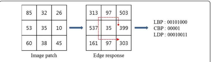
whereinandikare gray-level values of the surrounding pixels andk-th most significant directional response, respectively and the sign functions(x) is just as Equation (2). Figure1 shows the example of binary pattern containing LBP, CBP and LDP.
Gray level run length matrices
The Gary Level Run Length (GLRL) method is a way of extracting higher order statistical texture features [20]. This technique has been described and applied by Galloway and by Chu et al. A set of consecutive pixels with the same gray level, collinear in a given direction, constitutes a gray level run. The run length is the number of pixels in the run, and the run length value is the number of times such a run occurs in an image.
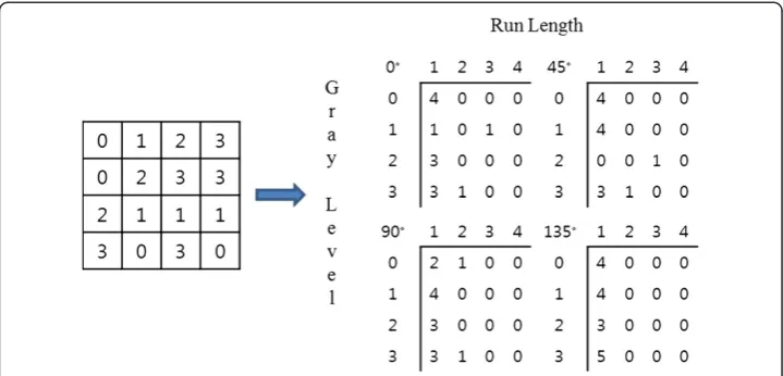
A Gray Level Run Length Matrix (GLRLM) is a two-dimensional matrix in which each elementp(i, j|θ) gives the total number of occurrences of runs of lengthjat gray leveli, in a given directionθ. Figure 2 shows a 4 × 4 picture having four gray levels (0–3) and the resulting gray level run length matrices for the four principal directions.
LetGbe the number of gray levels in the image, Rbe the longest run andn be the number of pixels in the image. In order to obtain numerical texture measures from the matrices, statistical texture features can be extracted from the GLRLM as follows:
1. Short Run Emphasis
SRE pð Þ ¼X G
i¼1 XR
j¼1
p ið;jjθÞ
j =
XG
i¼1 XR
j¼1
p ið;jjθÞ ð5Þ
Short Runs Emphasis (SRE) divides each run length value by the length of the run squared. This tends to emphasize short runs. The denominator is the total number of runs in the image and serves as a normalizing factor.
2. Long Runs Emphasis
LRE pð Þ ¼X G
i¼1 XR
j¼1
j2p ið;jjθÞ=X
G
i¼1 XR
j¼1
p ið;jjθÞ ð6Þ
Long Runs Emphasis (LRE) multiplies each run length value by the length of the run squared. This should emphasize long runs. The denominator is a normalizing factor, as above.
Proposed head pose estimation algorithm Random forests framework
A tree T in a forest F= {Ti} is built from the set of annotated patches P= {Pi= (Ii,ci)}
randomly extracted from the training images, where Ii and ci are the intensity of
patches and the annotated head pose class labels, respectively. Starting from the root, each tree is built recursively by assigning a binary Test ϕ (I)→{0, 1} to each non-leaf node. Such test sends each patch either to the left or right child, in this way the training patchesParriving at the node are split into two sets,PL(ϕ) andPR(ϕ).
The best test ϕ*is chosen from a pool of randomly generated ones ({ϕ}): all patches arriving at the node are evaluated by all tests in the pool and a predefined information gain of the splitIG(ϕ) is maximized:
ϕ¼Argmax
ϕIGð Þϕ ð7Þ
The process continues with the left and the right child using the corresponding train-ing sets PL(ϕ*) and PR(ϕ*) until a leaf is created when either the maximum tree depth is reached, or less than a minimum number of training samples are left [21].
Training
All the trees are trained on different training sets. These sets are generated from the original training set using the bootstrap procedure. For each training set, we randomly
select Ndata in the original set. The data are chosen with replacement. That is, some
data will occur more than once and some will be absent. Then, we randomly extract M patches with fixed size.
Our binary testsϕf,r,s,τ,type(I) are defined as:
f BPRLM rð ð ÞÞ−f BPRLM sð ð ÞÞ>τ; ð8Þ
wherefis the statistical texture feature,rands are pixel coordinate,τis a threshold,θ is the direction, typeis the type of Binary Pattern, andBPRLM(r) is the Binary Pattern Run Length Matrix (BPRLM) at gray levelI(r). During training, we use the different statistical texture feature, such as Short Run Emphasis and Long Run Emphasis, which is introduced in Section Random Forests. Short Run Emphasis tends to emphasize short runs, i.e., this feature represents the global texture measure. On the other hand, Long Run Emphasis tends to emphasize long runs, i.e., this feature represents the local texture measure. Therefore, we use Long Run Emphasis up to middle depth and then we use Short Run Emphasis.
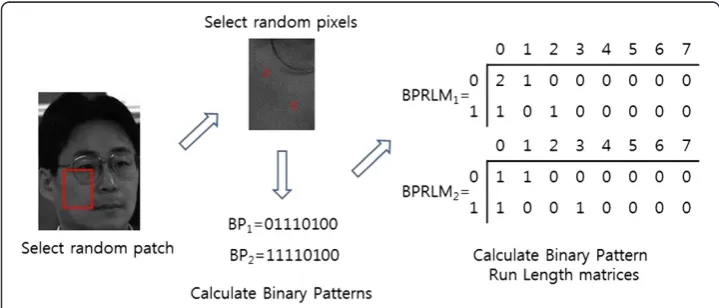
The Binary Pattern Run Length Matrix is the combination between the Binary Pattern and Run Length matrix, which can be calculated by the following steps. First, the binary patterns atI(r) andI(s) using predetermined binary pattern operator, such as LBP, CBP or LDP operator. Second, construct the Run Length matrices from the binary patterns in a direction 0°. Figure 3 shows an example of a Binary Pattern Run Length matrix using LBP operator.
During training, for each non-leaf node starting from the root, we generate a large pool of binary tests {ϕk} by randomly choosing f,r, s, τ, type. For efficiency reason, the number of binary tests is determined depend on the depth of the tree. That is, the number of the binary test increases with increasing the depth of the tree. The test
which maximizes a specific optimization function is picked. Our information gain IG
(ϕ) is defined as follows:
IGð Þ ¼ϕ Xi∈fL;Rgðμi−μÞ2− X
i∈fL;Rg ni
niþnj
Xni
j¼1 cij−μi
2
" #
; ð9Þ
whereniandμiare the number of samples and the mean of class at the child nodei, respectively, cijis the head pose class label of thej-thpatch contained in child node i, andμis the mean of class at the parent node. The information gainIG(ϕ)indicates the difference between the within variance and weighted between variance.
For each leaf, the class distributionp(ci|T) is stored. The distributions are estimated from
Testing
Given a new gray image of a head, patches that have the same size as the ones used for training are densely sampled from whole image and passed through all trees in the for-est. Each patch is guided by the binary tests stored at the nodes. A stride parameter controls how densely patches are extracted, thus easily steering speed and accuracy of the classification. At each node of a tree, the stored binary test evaluates a patch, send-ing it either to the right of left child, all the way down until a leaf. Arrivsend-ing at a leaf, a tree outputs the class distribution and the class label c that received the majority of votes. Because leaves with a low probability are not very informative and mainly add noise to the estimate, we discard all votes ifp(c|T) less than an empiric thresholdPmax. The
final class distribution is generated by arithmetic averaging of each remained distribution of all trees as follows:
p cðijFÞ ¼ F1 j j
Xj jF
t¼1
p cðijTtÞ ð11Þ
We choosecias the final class of an input image ifp(ci|F) has the maximum value.
Experiments
We evaluate the performance of our algorithm based on the CMU Multi-PIE database, which contains more than 750,000 images of 337 people recorded in up to four sessions over the span of five months. Subject were imaged under 15 view points and 18 illumination conditions while displaying a range of facial expressions [22]. In our paper, first ses-sion, 249 person, neutral expresses-sion, 18 illuminations and 7 view points, which consist of 0°, ±15°, ±30°, and ±45°, were employed. All of these face images were cropped to 32 × 32. Among these images, 50% were used for training and the rest for testing. Figure 4 shows an example of the CMU multi-PIE databases.
Training a forest involves the choice of several parameters. A set of values of parame-ters used for all experiments are given as follows. The patch dimension is 16 × 16 pixels;
the minimum patch number for split is 20 (m); the number of trees in the forest is
100 (Tmax); the maximum tree depth is 10 (Dmax); the number of training images for
each tree is 3,000 (n); the number of patch of each training image is 10; the
max-imum threshold is 0.5 (Pmax); the maximum number of binary test is 4000 tests, i.e.,
200 different combinations of f, r, s, type in Equation (8), each with 20 different
thresholdsτ.
In order to evaluate the performance of the proposed head pose estimation, we employed a combination of several methods. First, the Local Binary Pattern, Centralized
Binary Patterns, and Local Directional Pattern were employed for preprocessing. Second, Principal Component Analysis (PCA) and Linear Discriminant Analysis (LDA) were employed for feature extraction. Finally, a Support Vector Machine (SVM) was employed for the classifiers. In this experiment, 100 principal components are employed for PCA, Radial basis function (RBF) kernel is used for SVM.
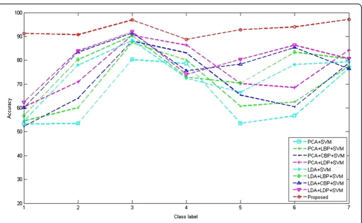
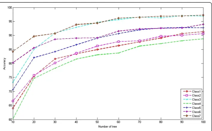
Table 1 shows the comparison results of the classification accuracies (CA) of the different algorithms. Because of the illumination change, the results of the LBP, CBP and LDP image were better than those of the raw images. Also, classification accuracy using LDP image showed better performance compared to other images transformed by binary pattern operators such as LBP and CBP. Furthermore, the proposed method has performance better than that of other methods, about 17% higher than that of LDP + PCA + SVM, and 13% higher than that of LDP + LDA + SVM. Figure 5 shows the comparison results of the classification accuracies of the different class. Furthermore, we summarized the classification accuracies in Table 2. As a result, maximum classification accuracies are 90.5%, 92.1%, and 97.2% when PCA + LDP + SVM, LDA + LDP + SVM, and proposed algorithm, respectively. Here, we can observe that proposed algorithm shows the less variance of classification accuracy than that of other algorithm. To further disclose the relationship between the recognition rate and the number of the trees, we showed the recognition results along with number of trees in Figure 6.
Table 1 Comparison of classification accuracies (CA) of different algorithms
Algorithm Raw image LBP image CBP image LDP image
PCA + SVM 64.6% 69.0% 70.3% 75.9%
LDA + SVM 73.9% 76.4% 78.7% 80.0%
Proposed 93.1% - -
Future works
Recently, 3D sensing devices have become available and computer vision researchers have started to leverage the additional depth information for solving some of the in-herent limitations of image-based methods. Even though depth sensors can solve much of the ambiguities inherent of standard video and even if their prices recently dropped, resolution of depth image is still low. Hence, the future work on head pose estimation could use color images in addition to depth data, as an RGB camera is available in the most common depth sensors.
Conclusion
In this paper we proposed to use a Binary Pattern Run Length matrix based on the ran-dom forests method for head pose estimation. In order to make this method robust in terms of illumination, the Binary Pattern Run Length matrix was employed; this matrix is the combination of a Binary Pattern and a Run Length matrix. Binary pattern is calculated using various operators, such as Local Binary Pattern, Centralized Binary Patterns, and Local Directional. In order to evaluate the discriminative power of the random tree method, a novel information gain was employed. Experiments on public databases show the advantages of this method over other algorithm in terms of ac-curacy and illumination invariance.
Table 2 Comparison of classification accuracies (CA) of different class
Algorithm Class1 Class2 Class3 Class4 Class5 Class6 Class7
PCA + LDP + SVM 60.4% 70.9% 90.5% 86.4% 70.2% 68.5% 84.3%
LDA + LDP + SVM 62.4% 84.0% 92.1% 74.5% 80.4% 86.7% 80.6%
Proposed 91.3% 90.6% 96.8% 88.7% 92.7 93.9% 97.2%
Competing interests
The authors declare that they have no competing interest.
Authors’contributions
HDK and SHL conceptualized the core functions of head pose estimation algorithm and drafted the manuscript. MKS and DJK conducts the implementation including algorithm design, experiments and acquisition of evaluation data. All authors read and approved the final manuscript.
Acknowledgement
This work was supported by the DGIST R&D Program of the Ministry of Education, Science and Technology of Korea (14-IT-03). It was also supported by Ministry of Culture, Sports and Tourism (MCST) and Korea Creative Content Agency (KOCCA) in the Culture Technology (CT) Research & Development Program (Immersive Game Contents CT
Co-Research Center).
Received: 2 February 2014 Accepted: 26 April 2014
References
1. Murphy-Chutorian E, Trivedi MM (2009) Head pose estimation in computer vision: a survey. IEEE Trans Pattern Anal Mach Intell 607:626
2. Gee A, Cipolla R (1994) Determining the gaze of faces in images. Image and Vision Computting 639:647 3. Li Y, Wang S, Ding X (2010) Person-independent head pose estimation based on random forest regression. IEEE
Int Conf Image Processing 1521:1524
4. Huang C, Ai H, Li Y, Lao S (2007) High-performance rotation invariant multiview face detection. IEEE Trans Pattern Anal Mach Intell 671:686
5. Raytchev B, Toda I, Sakaue K (2004) Head pose estimation by nonlinear manifold learning. IEEE Int Conf Pattern Recognition 462:466 (204)
6. Li Y, Gong S, Liddell H (2000) Support vector regression and classification based mult-view face detection and recognition. IEEE Int Conf Automatic Face and Gesture Recognition 300:305
7. Fanelli G, Gall J, Van Gool L (2011) Real time head pose estimation with random regression forests. IEEE Int Conf Computer Vision and Pattern Recognition 617:624
8. Breiman L (2001) Random Forests. Machine learning. 5:32
9. Vatahska T, Bennewitz M, Behnke S (2007) Feature-based head pose estimation from images. IEEE-RAS Int Conf Humanoid Robots 330:335
10. Whitehill J, Movellan JR (2008) A discriminative approach to frame-by-frame head pose tracking. IEEE Int Conf Automatic Face and Gesture Recognition 1:7
11. Yao J, Cham WK (2004) Efficient model-based linear head motion recovery from movies. IEEE Int Conf Computer Vision and Pattern Recognition 414:421
12. Morency LP, Whitehill J, Movellan JR (2008) Generalized adaptive view-based appearance model: integrated framework for monocular head pose estimation. IEEE Int Conf Automatic Face and Gesture Recognition 1:8 13. Balasubramanian VN, Ye JP, Panchanathan S (2008) Biased manifold embedding: a framework for
person-independent head pose estimation. IEEE Int Conf Computer Vision and Pattern Recognition 1:7 14. Huang D, Storer M, De la Torre F, Bischof H (2011) Supervised local subspace learning for continuous head pose
estimation. IEEE Int Conf Computer Vision and Pattern Recognition 2921:2928
15. Osadchy M, Miller ML, LeCun Y (2007) Synergistic face detection and pose estimation with energy-based models. Mach Learning Research 1197:1215
16. Huang C, Ding XQ, Fang C (2010) Head pose estimation based on random forests for multiclass classification. IEEE Int Conf Computer Vision and Pattern Recognition 934:937
17. Ojala T, Pietkainen M, Maenpaa T (2002) Multiresolution gray-scale and rotation invariant texture classification with local binary patterns. IEEE Trans Pattern Anal Mach Intell 971:987
18. Fu X, Wei W (2008) Centralized binary patterns embedded with image Euclidean distance for facial expression recognition. IEEE Int Conf Natural Computation 115:119
19. Jabid T, Kabir MH, Chae O (2010) Robust facial expression recognition based on local directional pattern. J ETRI 784:794 20. Galloway MM (1975) Texture analysis using gray level run lengths. Computer Graphics and Image Processing
172:179
21. Fanelli G, Danotone M, Gall J, Fossati A, Van Fool L (2013) Random forests for real time 3D face analysis. International J of Computer Vision 437:458
22. Gross R, Matthews I, Cohn JF, Kanade T, Baker S (2010) Multi-PIE. Image Vis Comput 807:813
doi:10.1186/s13673-014-0009-7