R E S E A R C H
Open Access
Image contour based on context aware in complex
wavelet domain
Nguyen Thanh Binh
Correspondence: [email protected]
Faculty of Computer Science and Engineering, Ho Chi Minh City University of Technology, Ho Chi Minh, Vietnam
Abstract
Active contours are used in the image processing application including edge detection, shape modeling, medical image-analysis, detectable object boundaries, etc. Shape is one of the important features for describing an object of interest. Even though it is easy to understand the concept of 2D shape, it is very difficult to represent, define and describe it. In this paper, we propose a new method to implement an active contour model using Daubechies complex wavelet transform combined with B-Spline based on context aware. To show the superiority of the proposed method, we have compared the results with other recent methods such as the method based on simple discrete wavelet transform, Daubechies complex wavelet transform and Daubechies complex wavelet transform combined with B-Spline.
Keywords:Daubechies complex wavelet transform; Context-awareness; Active contour
Introduction
Contours are used extensively in image processing applications. Active contours can be classified according to several different criteria. One of the classifications is based on the flexibility of the active contour and is proposed in a slightly modified form by Jain [1]. The active contour models can be accordingly partitioned in two classes: free form of active contour models and limited form of active contour models.
The free form of active contour models constrained by local continuity and smooth-ness constraints [2–7]. Its limit uses a priori information about the geometrical shape directly. This information is available in the form of a sketch or a parameter vector that encodes the shape of interest. The geometric shape of the contour is adjusted by varying the parameters [8–13]. They cannot take any arbitrary shapes.
The snake has found wide acceptance and has proven extremely useful in the appli-cations for medical analysis, feature tracking in the video sequences, three-dimensional object recognition [14], and stereo matching [15]. To take active contour, there are many methods to take it.
In the past, many algorithms have been built to find object contour. The dual-tree Complex Wavelet Transform (DTCWT) was proposed by Kingsbury [16]. In DTCWT, he used two trees of real filters for the real and imaginary parts of the wavelet coeffi-cients. Recently, Bharath [17] has presented a framework for the construction of steer-able complex wavelet.
This transform also avoids the shortcomings of discrete wavelet transform, but it uses a non-separable and highly redundant implementation. The redundancy of this trans-form is even higher than that of DTCWT.
In the entire complex transforms above, use of real filters make them not a true com-plex wavelet transform and due to the presence of redundancy, they are computationally costly. Lawton [18] and Lina [19] used an approximate shift-invariant Daubechies com-plex wavelet transform for avoiding redundancy and providing phase information. Shensa [20] and Ansari [21] use Lagrange filters, Akansu [22] uses binomial filters. Shen [22] used the Daubechies filter roots. Goodman [23] considered them as the roots of a Laurent polynomial. Temme [24] described the asymptotic of the roots in terms of a representa-tion of the incomplete beta funcrepresenta-tion. Almost of that method related Daubechies filters.
The wavelet transform for contour has serious disadvantages, such as shift-sensitivity [25] and poor directionality [26]. Several researchers have provided solutions for min-imizing these disadvantages. Some of them have suggested the other method such as: local binary fitting [27, 28], local region descriptors [29], local region [30], local region based [31], local intensity clustering method. There exist some drawbacks with local re-gions. In [32], the problem is how to define the degree of overlap.
The local region based method has two drawbacks: (i) the Dirac functional is re-stricted to a neighborhood around the zero level set. (ii) Region descriptors only based on regions mean information without considering region variance [33].
Use of complex-valued wavelet can minimize these disadvantages. The DCWT uses complex filters and can be made symmetric, thus leading to symmetric DCWT, and it is more useful for image contour.
In this paper, we propose a new method to implement an active contour model using Daubechies complex wavelet transform combined with B-Spline based on context-aware (DCWTBCA). To show the superiority of the proposed method, we have compared the results with the other recent methods such as the method based on simple discrete wave-let transform (DWT), Daubechies complex wavewave-let transform (DCWT) and Daubechies complex wavelet transform combined with B-Spline (DCWTB). The rest of the paper is organized as follows: in section 2, we described the basic concepts of Daubechies complex wavelet transform. Details of the proposed algorithm have been given in section 3. In sec-tion 4, the results of the proposed method for contour have been shown and compared with other methods. Finally in section 5, we presented our conclusions.
Background
In this section, we present the theory related to the work such as: Complex Daubechies Wavelet and advantages of B-Spline for Snakes.
Construction of complex Daubechies wavelet
The basic equation of multiresolution theory [34-37,38] is the scaling equation:
φð Þ ¼x 2X
k
akφð2x−kÞ ð2:1Þ
where,akare the coefficients. Theakcan be real as well as complex valued and∑ak= 1.
Daubechies wavelet bases {ψj,k(t)} in one dimension are defined through the above scaling
Forφ(x) to be Daubechies scaling function the following conditions must be satisfied [39, 40]:
(i)Compactness of the support ofφ: It requires thatφ(and consequentlyψ) has a compact support inside the interval[−J, J + 1]for the integerJ, that is,ak≠0for k =−J,−J + 1,…., J, J + 1
(ii)Orthogonality of theφ(x-k): This condition defines in a large sense the Daubechies wavelets. Defining the polynomial
F zð Þ ¼X Jþ1
n¼−J
anzn; with Fð Þ ¼1 1;j j ¼z 1 ð2:2Þ
wherez is on the unit circle, the orthonormality of the set {φ0,k(x),k∈Z} can be stated
through the following identity
P zð Þ−Pð Þ ¼−z z ð2:3Þ
where the polynomial P(z) is defined as
P zð Þ ¼zF zð ÞF zð Þ ð2:4Þ
(iii)Accuracy of the approximation: To maximize the regularity of the functions generated by the scaling functionφ, we require the vanishing of the firstJmoments of the wavelet in terms of the polynomial Eq. (2.2)
F0ð Þ ¼−1 F}ð Þ ¼−1 ::::::¼Fð ÞJð Þ ¼−1 0 ð2:5Þ (iv)Symmetry: This condition amounts to haveak= a1-kand can be written as
F zð Þ ¼zF z−1 ð2:6Þ
As anticipated by Lawton [18], only complex-valued solutions ofφ andψ, under the
four constraints above, can exist and for evenJonly. The first solutions (fromJ = 0to J = 8) were described in [32] by using the parameterized solutions of Eq. (2.3), (2.5) and (2.6). The solutions have also been investigated in the spirit of the original Daubechies approach, i.e. by inspection of the roots of a so-called“valid polynomial”that satisfies Eq. (2.4). Such a polynomial is defined as
PJð Þ ¼z
1þz 2 2Jþ2
pJ z−1 ð2:7Þ
where
pJð Þ ¼z X 2J
j¼0
rjðzþ1Þ2J−jðz−1Þj
with
r2j¼ð Þ−1 j2−2J
2Jþ1 j
r2jþ1¼0
; j¼0;1; ::::;J 8
<
: ð2:8Þ
The 2J roots ofpJ(z) display obvious symmetries: the conjugate and the inverse of a
root are also roots; furthermore, no root is of unit modulus. If we denote by xk (k =
1,2,…….J), the roots inside the unit circle(|xk| < 1)then
pJð Þ ¼z Y
J
k¼1 z−xk
1−xk
YJ k¼1
z−xk−1
1−xk−1
ð2:9Þ
and the low-pass filterF(z)can be written as:
F zð Þ ¼ 1þz 2
1þJ
p z−1
With
p zð Þ ¼Y
m∈R
z−xm
1−xm
Y
n∈R0
z−x−1
n
1−x−1
n
ð2:10Þ
where R, R’ are two arbitrary subsets of {1, 2, 3,…,J}. The spectral factorization of P zð Þ ¼zF zð ÞF zð Þ implies pJð Þ ¼z zJp zð Þ−1 p zð Þ which leads to the following con-straint on R and R’:
k∈R⇔k∉R0 ð2:11Þ
This selection of root fulfills the conditions (i), (ii) and (iii). The addition of the sym-metry condition (iv) defines a subset of solutions of Eq. (2.11). It corresponds to the constraint
k∈R⇔J−kþ1∈R0 and k∉R0
For any even value of J, this defines a subset of2J/2complex solution in the original set of“Daubechies wavelets”. A complex conjugate of a solution is also a solution.
Properties of Daubechies complex wavelet
Daubechies Complex Wavelet has important properties [26, 39]:
(i)Symmetry and linear phase property:
The nonlinear phase distortion was precluded by the linear phase response of the filter. It keeps the shape of the signal. This is very important in image processing. (ii) Relationships between real and imaginary components of the scaling and the
wavelet functions.
(iii)Multiscale edge Information
Advantages of B-Spline for snakes
In computer graphics, there are two splines which usually used: B-Splines and Bezier Splines. However, B-Splines have two advantages over Bezier Splines [41]: the number of control points can be set independently to the degree of a B-Spline polynomial and B-Splines allow local control over the shape of a Spline curve. From the advantages above of B-Splines, we choose B-Splines for our proposed method.
The important of constructing a snake is convenient to choose a set of control points on the image than to connect the point with straight lines. The B-Spline basis for snakes on the following:
(i) B-splines are piecewise polynomial that makes them very flexible. (ii) B-splines can be make smooth curve.
(iii) B-splines preserve the shape that a spline has the same shape as its control polygon or more precisely.
Advantages of DCWT for active contour
In the past, many algorithms have been built to process image by DWT. DWT has three serious disadvantages [26]: shift sensitivity, poor directionality and lack of phase information. We can use DCWT to reduce these disadvantages. On the basis of Daubechies complex wavelet, we have the following advantages for the ac-tive contour:
(i) Symmetric and linear phase property of DCWT can keeps the shape of the signal and carries strong edge information. The linear phase response of the filter precludes the nonlinear phase distortion and keeps the shape of the signal and it reduces the misleading and deformed shape of objects.
(ii) DCWT can act as the local edge detectors. The imaginary and real components represent strong edges. This helps in preserving the edges and implementation of edge-sensitive contour methods.
(iii) DCWT has reduced shift sensitivity. DCWT reconstructs all local shifts and orientations in the same manner. So, it is clear that it can quickly find the boundary of objects.
The proposed method for image contour
This section describes the proposed method for contour objects. The term‘context-aware’ [42] refers to context as locations, identities of nearby people and objects, and changes to those objects.
Most of previous definitions of context are available in literature [43] that context-aware looks at who’s, where’s, when’s and what’s of entities and uses this information to determine why the situation is occurring. Here, our definition of context is:
In image processing, if a piece of information can be used to characterize the situ-ation of a participant in an interaction, then that informsitu-ation is context. Contextual information can be stored in feature maps on themselves. Contextual information is collected over a large part of the image. These maps can encode high-level semantic features or low-level image features. The low-level features are image gradients, texture descriptors and shape descriptors information [42, 44].
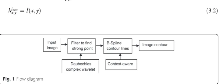
The proposed algorithm is of three steps: preprocessing of images, Daubechies com-plex wavelet filter bank and context- aware closed contour with boundary information. The goal of the second step is to detect the dominant edge points so that the resulting image will be composed of textures separated by the edges. We use Daubechies com-plex wavelet transform for edge detection that can act as the local edge detectors. The imaginary components of complex wavelet coefficients represent strong edges. Using a threshold parameter weak edges is wiped out. It works as a structure preserving noise removal process as well. Since we need to find the coordinates of the edges after this process, we use contour lines for that purpose since they provide closed edge curves which will ease the process when computing in the wavelet domain. Here, we use B-Spline contour lines. Steps of the proposed method are as follows in Fig. 1:
Firstly, preprocessing of images. The collected images are scale normalized to 256 × 256 pixel, 512 × 512 pixel dimensions in order to reduce complexity.
Secondly, Daubechies complex wavelet filter bank. For Daubechies complex filter bank computation in the proposed method, Daubechies decomposition proceeds through two main periods: reconstruction of the signal from the coefficients and energy formula-tion to define strong point.
Finally, context- aware closed contour with boundary information. Here, we use B-Spline contour lines, which covers the object.
Reconstruction of the signal from the coefficients
According to the multi-resolution analysis with tensor product bases, an image f(x, y) is
projected onto some “approximation” spaces generated by the dyadic translations of
the scaled function φ(x) andφ(y) (at the resolution scale jmax of the original image). If we denote the complex projection coefficients by
cjmax
x;y ¼hjxmax;y þigjxmax;y ð3:1Þ
then we can estimatehjmax
x;y andg jmax
x;y with the following steps of the iterative procedure:
1. Start from the usual approximation:
hjmax
x;y ¼I xð ;yÞ ð3:2Þ
Input image
Filter to find strong point
B-Spline
contour lines Image contour
Daubechies complex wavelet
Context-aware
2. Evaluatehjmaxþ1
x;y using a one-level synthesis operation with the real part of the
inverse symmetric Daubechies wavelet kernel only.
3. Make a one-level complex wavelet transform. The result is a quite accurate estimation of the real and imaginary parts of the projection coefficientcjmax
x;y . In the
first approximation,
hjmax
x;y ≅I xð ;yÞ ð3:3Þ
andgjmax
x;y is proportional to the Laplacian of thef(x, y).
AN-level wavelet transformWcan be represented as
cjmax
x;y
n o
→W cjmax−N
x;y ; dxjmax;y−N; :::: djxmax;y−1
n o
ð3:4Þ where the quantities djmax−k
x;y represent the set of coefficients for the three wavelet
sec-tors. The complex scaling wavelet coefficients cjmax−N
x;y result from the nested actions of
the complex low-pass filter.
To solve the snake problem numerically, we express its cubic Spline solution using the standard B-Spline expansion
sð Þ ¼x X
k∈Z
c kð Þβ3ðx−kÞ ð3:5Þ
where c(k) are the Spline coefficients, and the generating function is the cubic B-Spline given by
β3 x
ð Þ ¼ 2=3þj jx
3=2−x2; 0≤j jx <1 2−j jx
ð Þ3=
6; 1≤j jx <2
0; 2≤j jx
8 <
: ð3:6Þ
Using the basic convolution and differentiation rules of Splines [45], we obtain the explicit formula
ξð Þ ¼s X
k∈Z
V k ;b31cð Þk þλX
k∈Z
b31dð Þ2 c
k
ð Þ dð Þ2 c
k
ð Þ ð3:7Þ
where * denotes the discrete convolution operator and the kernels b13(discrete cubic B-spline) and d(2) (second difference) are defined by their z-transform as follows [45]:
B3
1ð Þ ¼z ðzþ4þz−1Þ=6 andD
(2)
(z) =z−2 +z−1 (3.8)
We have now replaced the integral in the second term by a sum, which is much more computationally tractable. The task is then to minimize Eq. (3.7), which is typically achieved by differentiation with respect to c(k).
The argument is essentially the same for more general curves in the plane, which are described using two Splines instead of one. Specifically, we represent a general B-Spline snake as follows:
shð Þ ¼t sxð Þt ;syð Þt
¼X k∈Z
c kð Þ:βn t h−k
0≤t≤tmax¼hN ð3:9Þ
where sx(t) and sy(t) are the x and y Spline components, respectively; these are both parameterized by the curvilinear variable. The exact value of tmax, which marks the end of the curve, is dictated by the desired resolution of the final discrete curve; by convention, we do only render the curve points for t integer. This 2D Spline snake is characterized by its vector-sequence of B-Spline coefficients c(k) = (cx(k), cy(k)). Note that there are only N = tmax/h primary coefficient vectors, each corresponding to a Spline knot on the curve; the other coefficient values are deduced using some pre-scribed boundary conditions. Clearly, if we specify N, the above automatically defines the knot spacing h and therefore the smoothness constraint for the curve.
Assuming a curve representation by M = tmax discrete points, we obtain h = M/ N. The freedom of the Spline curve has been reduced by the same amount, result-ing in a smoothresult-ing and stiffenresult-ing of the curve. Increasresult-ing the number N of node points will reduce the knot spacing, and consequently it will reduce the smoothing effect of the curve.
Energy formulation
The external potential function is typically given by a smoothed version of the gradient of the input data [45, 46]
g xð ;yÞ ¼
ffiffiffiffiffiffiffiffiffiffiffiffiffiffiffiffiffiffiffiffiffiffiffiffiffiffiffiffiffiffiffiffiffiffiffiffiffiffiffiffiffiffiffiffiffiffiffiffiffiffiffiffiffiffi
∂ ∂xφf
2
þ ∂∂
yφf
2
s
ð3:10Þ
where f denotes the input image and φis a smoothing kernel; for example, a Gaussian. Our cost function is the summation of the gradient (external force) over the path of the curve s(x) sampled at M consecutive points
ξðc kð ÞÞ ¼X
M−1
i¼0
−g s iðð ÞÞ ð3:11Þ
For the cost function to be a good approximation of the curvilinear integral, we typic-ally select M sufficiently large so that the curve points are connected (i.e., within a dis-tance of one pixel of each other). However, we note that the exact value of M is not critical; a less dense sampling may be used to increase optimization speed. The negative sign in Eq. (3.11) is used because we employ a minimization technique for the optimization.
s ið Þ ¼X
k∈Z
c kð Þ:βn i h−k
; h¼M
N ð3:12Þ
Below, we present two different ways for fast curve rendering by digital filtering. (i) Interpolation: The most straightforward way is interpolation. The B-Spline func-tion is evaluated at every posifunc-tion (i/h - k) multiplied by the corresponding B-Spline co-efficient and summation. B-Splines are of compact support, and therefore, the summing needs only to be carried out over a subset of all coefficients. To interpolate the curve at a point i, only the coefficients c(k)
i h−
nþ1 2
≤k≤ i hþ
nþ1 2
ð3:13Þ
need to be included in the sum ( [.] denotes integer truncation).
The main computational drawback of this procedure is that the function Eq. (3.6) needs to be evaluated for each term in the sum.
(ii) Digital Filtering: The above described algorithm works for any combination of values of M and N. If we can impose M such that h is an integer value, a much more efficient algorithm can be described. In general, this requirement is easily met, it is not critical and can be loosely chosen. The simplification is based on a convolution prop-erty for B-Splines [45]. It states that any Spline of degree n and knot spacing h (integer) can be represented as the convolution of n + 1 moving average filters of size h followed by a Spline of knot spacing one. Hence, three successive steps can obtain the curve points:
Up-sampling of the B-Spline coefficients;
Averaging by (n + 1) moving average filters of size h; Filtering by a unit B-Spline kernel of degree n.
This algorithm can be implemented with as few as two multiplications and two addi-tions per node point plus (2n) addiaddi-tions per computed contour coordinate. Generally, it is faster and also at least a factor of two better than the Oslo knot insertion algorithm commonly used in the computer graphics.
Border conditions
Appropriate boundary conditions are necessary for the computation of Eq. (3.9) and Eq. (3.10) [45]. In the following, we distinguish the cases of a close snake and an open snake.
(i) Close Snake Curve: For a set of node points n(k), k = 0,1,…., N-1 we require that n(N) = n(0) and n(−1) = n(N-1). The corresponding boundary conditions are periodic. The extended signalns(k)of infinite length can be described as
nsð Þ ¼k n kð modNÞ ð3:14Þ
These anti-mirror conditions are such that
n k0ð þkÞ−n k0ð Þ
ð Þ ¼ðn kð Þ0 −n k0ð −kÞÞ ð3:15Þ where k0 Є {0, N-1}. Since the extended signal has a center of anti-symmetry at the boundary value, this value will be preserved exactly whenever the filter applied is sym-metric, which turns out to be the case here. However, a new boundary value cannot be defined as the lookup of an existing signal value, which makes the implementation slightly more complicated.
From Fig. 2 and many cases of the other image tests, we observed that the proposed method accurately detects contour.
Experiments and results
To demonstrate the validity of the proposed method, we have tested on many images. We have compared the results with the other recent methods such as the method based on simple discrete wavelet transform (DWT), and the Daubechies complex wave-let transform (DCWT), the Daubechies complex wavewave-let transform combined with B-Spline (DCWTB) and the proposed method using the Daubechies complex wavelet transform combined with B-spline based on context aware. These methods were imple-mented on our matlab program and comparison has been made on the same images and on the similar scale. In our approach, we have taken dataset images for testing. This data set has 600 images. The proposed method was tested on different cases.
(a)
(b)
(c) (d)
To test our algorithm, many images of different sizes have been used. We compare the proposed method on two cases: strong objects and weak objects. The strong object is defined as an object whose boundaries are clear and the weak object is defined as an object whose boundaries are blurred. We have experimented on several images and here we report on some selected images.
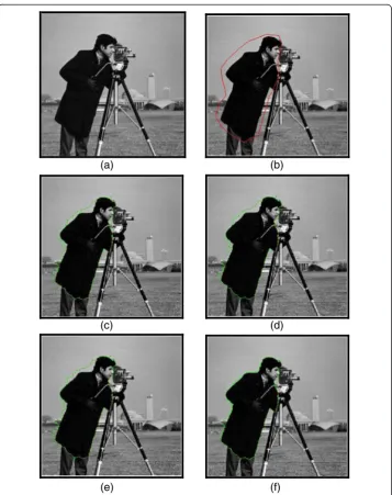
As shown in Fig. 3, for the Cameraman image, we select an object. In this case, the object is Cameraman body (strong object) as Fig. 3(b). The results of DWT, DCWT and DWTB method are shown in Fig. 3(c), (d) and (e). The result of the proposed method is shown in Fig. 3(f ). Here it can be observed that the result in Fig. 3(f ) is better than the result in Fig. 3(c), (d), (e) at the same number of iterations (600 iterations).
(a) (b)
(c) (d)
(e) (f)
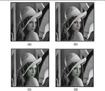
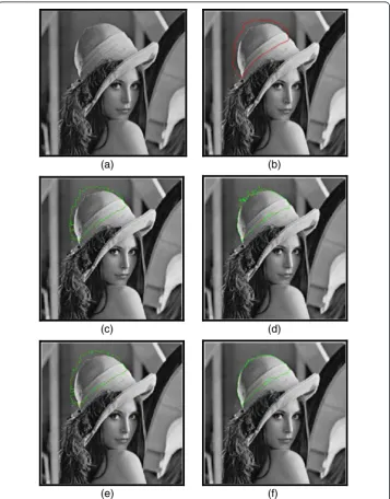
Similarly, as shown in Fig. 4, for the Lena image, we select an object. In this case, the
object is Lena’s hat (strong object) as Fig. 4(b). The results of DWT, DCWT and DWTB
method are shown in Fig. 4(c), (d) and (e). The result of the proposed method is shown in Fig. 4(f ). Here it can be observed that the result in Fig. 4(f ) is better than the result in Fig. 4(c), (d), (e) at the same number of iterations (400 iterations).
We tested the proposed method on a set of several images and compared with the other methods. From Figs. 3, 4 and many other tests, we observed that, in the case of strong objects, the proposed method is better than the other methods.
(a) (b)
(c) (d)
(e) (f)
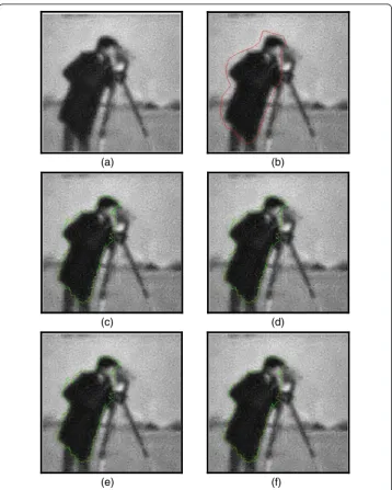
We now apply the proposed method with the weak objects cases. The weak objects are the objects with less clear boundaries. The important edge site is blurred in the ob-ject; therefore, the boundaries become obscure, thereby misleading the curve deform-ing. Weak objects have less clear boundaries, the extraction of weak object is not easy work. As a result, weak object could not be extracted precisely.
In Fig. 5, we select the Cameraman body (weak object) image as Fig. 5(b). The Fig. 5(a) is Cameraman original image. Heavy blur and noise has been added in this image to make the object weak. The results of DWT, DCWT and DWTB method are shown in Fig. 5(c), (d) and (e). The result of the proposed method is shown in Fig. 5(f ). Here it
(a) (b)
(c) (d)
(e) (f) Fig. 5Performance of the proposed method on Cameraman image compared to the DWT based method
can be observed that the result in Fig. 5(f ) is better than the result in Fig. 5(c), (d), (e) at the same number of iterations (600 iterations). In contour classification, the goal is to assign an object into one of a set of predefined set of contour classes. The classification is performed by using a subset of the sub-band energies that are measured to produce a feature vector that describes the contour.
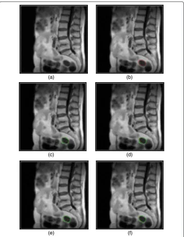
Figure 6 also compares the proposed algorithm with other methods on an image that comprises the object with weak edge (blurred image). The results shown in Fig. 6(f ) is better than the results shown in Fig. 6(c), (d) and (e) at the same number of 450
(a) (b)
(c) (d)
(e) (f)
iterations. Therefore, we can say that the performance of the proposed method is better than other methods in case of weak objects.
To sum up, from all the above experiments and many other experiments, we ob-serve that the performance of the proposed method is better than the DWT based method in the both cases: weak objects and strong objects. However, in the case of weak objects, they have less clear boundaries, the extraction of weak object is not easy work.
The symmetry and linear phase property is one of the reasons why the Daubechies complex wavelet performs better than other methods. The proposed method keeps the shape of the signal and carries strong edge information. It prevents the deformation of object boundaries. Therefore, it is helpful to find edges of an object in image. On the other hand, DCWT has reduced shift sensitivity. As the contour moves through space, the reconstruction using real valued discrete wavelet transform coefficients changes erratically, while complex wavelet transform reconstructs all local shifts and orienta-tions in the same manner. Therefore, it is clear that it can quickly find boundaries of an object.
Conclusions
In this paper, the image contour model with Daubechies complex wavelet transform combined with B-Spline based on context-aware is proposed. The proposed technique allows estimating the contour location of a target object along an image. The contribu-tion in the use of Daubechies complex wavelet transform for image was discussed. Mathematical basis of the Daubechies complex wavelet transform and B-Spline proved that image features based on the wavelet transform coefficients can be used very effi-ciently for image contour classification.
From the results shown in the above section, we see that the proposed method per-forms better in case of both strong and weak objects. The proposed method can be ap-plied on any modality of images. However, in the case of weak objects, the proposed method finds approximate boundaries. Therefore, if the quality of the image is very bad due to heavy noise or heavy blur, etc., then the estimation ability is reduced because of the effect to edge the object. To avoid this problem, we can reduce noise and blur before applying the proposed method. In the future work, the method is going to be compared with some other methods to evaluate its results in different cases and the complexity of them.
Competing interests
The authors declare that they have no competing interests.
Authors' information
Nguyen Thanh Binh received the Bachelor of Engineering degree from Ho Chi Minh City University of Technology, Vietnam, the Master's degree and Ph.D degree in computer science from University of Allahabad, India. Now, he is a lecturer at Faculty of Computer Science and Engineering, Ho Chi Minh city University of Technology- Vietnam National University in Ho Chi Minh City. His research interests include recognition, image processing, multimedia information systems, decision support system, time series data.
Acknowledgment
The author is grateful to the valuable guidance provided by Dr. Ashish Khare, Department of Electronics and Communication, University of Allahabad, India.
References
1. Jain AK, Zhong Y, Lakshmanan S (1996) Object Matching Using Deformable Templates. IEEE Transactions on Pattern Analysis and Machine Intelligence 18(3):267–278
2. Kass M, Witkin A, Terzopoulos D (1988) Snakes: Active contour models, International Journal of Computer Vision, 1(4):321–331, ISSN 0920-5691. http://link.springer.com/article/10.1007/BF00133570
3. Szekely G, Kelemen A, Brechbuhler C, Gerig G (1996) Segmentation of 2-D and 3-D objects from MRI volume data using constrained elastic deformations of flexible Fourier contour and surface models. Med Image Anal 1(1):19–34
4. Lewis FL, Gurel A, Bogdan S, Doganalp A, Pastravanu OC, Wong YY, Yuen PC, Tong CS (1998) Segmented snake for contour detection. Pattern Recogn 31(11):1669–1679
5. Gunn SR, Nixon MS (1998) Global and local active contours for head boundary extraction. Int J Comput Vis 30(1):43–54 6. Garrido A, Blanca DL (1998) Physically-based active shape models: initialization and optimization. Pattern Recogn
31(8):1003–1017
7. Blake A, Isard M (1998)“Active contours”, Springer
8. Chuang JH (1996) A potential-based approach for shape matching and recognition. Pattern Recogn 29(3):463–470 9. Chakraborty A, Staib LH, Duncan JS (1994) Deformable boundary finding influenced by region homogeneity,
Proceedings of IEEE Computer Society conference on Computer Vision and Pattern Recognition (CVPR), pp. 624–627
10. Cootes TF, Taylor CJ, Cooper DH, Graham J (1995) Active shape models-their training and application. Comput Vis Image Underst 61(1):38–59
11. Yuille AL, Cohen DS, Hallinan PW (1989) Feature extraction from faces using deformable templates, Proceedings of IEEE Computer Society Conference on Computer Vision and Pattern Recognition, pp. 104–109
12. Amit Y, Grenander U, Piccioni M (1991) Structural image restoration through deformable templates. J Am Stat Assoc 86(414):376–387
13. Lakshmanan S, Grimmer D (1996) A deformable template approach to detecting straight edges in radar images. IEEE Transactions on Pattern Analysis and Machine Intelligence 18(4):438–442
14. Wang JY, Cohen FS (1994) Part II: 3-D object recognition and shape estimation from image contours using B-splines, shape invariant matching, and neural networks, IEEE Transactions on Pattern Analysis and Machine Intelligence, vol. 16, no. 1, pp. 13–23
15. Menet S, Marc PS, Medioni G (1990) B-snakes: Implementation and application to stereo, Image Understanding Workshop, pp. 720–726
16. Kingsbury NG (1999) Image processing with complex wavelets, Philosophical Transactions of Royal Society London. Ser A 357:2543–2560
17. Bharath AA, Ng J (2005) A Steerable Complex Wavelet Construction and Its Application to Image Denoising, IEEE Transactions on Image Processing, vol. 14, no. 7, pp. 948–959
18. Lawton W (1993) Applications of complex valued wavelet transform in sub band decomposition. IEEE Trans Signal Process 41(12):3566–3568
19. Lina JM, Mayrand M (1995) Complex Daubechies Wavelets. Journal of Applied and Computational Harmonic Analysis 2:219–229
20. Shensa MJ (1992) The discrete wavelet transform: wedding the á trous and Mallat algorithms. IEEE Trans Signal Process 40(10):2464–2482
21. Ansari R, Guillemot C, Kaiser JF (1991) Wavelet construction using Lagrange halfband filters. IEEE Transactions on Circuits and Systems 38(9):1116–1118
22. Akansu AN, Haddad RA, Caglar H (1993) The binomial QMF-wavelet transform for multiresolution signal decomposition. IEEE Trans Signal Process 41(1):13–19
23. Shen J, Strang G (1996) The zeros of the Daubechies polynomials. Proc Am Math Soc 124:3819–3833 24. Goodman TNT, Micchelli CA, Rodriguez G, Seatzu S (1997) Spectral factorization of Laurent polynomials. Adv
Comput Math 7(4):429–454
25. Candes EJ (1998) Ridgelets: Theory and Applications, PhD thesis, Stanford University. http://statweb.stanford.edu/~candes/ papers/Thesis.ps.gz
26. Khare A, Tiwary US (2006) Symmetric Daubechies Complex Wavelet Transform and its application to Denoising and Deblurring. WSEAS Transactions on signal processing 2(5):738–745
27. Li C, Kao C, Gore JC, Ding Z (2008) Minimization of Region-Scalable Fitting Energy for Image Segmentation. IEEE Trans Image Process 17:1940–1949
28. Li C, Kao C, Gore J, Ding Z (2007), Implicit Active Contours Driven by Local Binary Fitting Energy, IEEE Conference on Computer Vision and Pattern Recognition, pp 1–7, ISSN:1063-6919 http://ieeexplore.ieee.org/xpl/login.jsp?tp= &arnumber=4270039&url=http%3A%2F%2Fieeexplore.ieee.org%2Fxpls%2Fabs_all.jsp%3Farnumber%3D4270039 29. Darolti C, Mertins A, Bodensteiner C, Hofmann U (2008) Local Region Descriptors for Active Contours Evolution.
IEEE Trans Image Process 17:2275–2288
30. Brox T, Cremers D (2009) On Local Region Models and a Statistical Interpretation of the Piecewise SmoothMumford-Shah Functional. Int J Comput Vis 84:184–193
31. Lankton S, Tannenbaum A (2008) Localizing Region-Based Active Contours. IEEE Trans Image Process 17:2029–2039
32. Lawton WM (1991) Necessary and sufficient conditions for constructing orthonormal wavelet bases. J Math Phys 32(1):57–61 33. Li C, Huang R, Ding Z, Gatenby C, Metaxas D, Gore JC (2011) A Level Set Method for Image Segmentation in the
Presence of Intensity Inhomogeneity with Application to MRI. IEEE Trans Image Process 20:2007–2016 34. Strang G (1992) The optimal coefficients in Daubechies wavelets. Physical D: Nonlinear phenomena 60:239–244 35. Lina JM, Mayrand M (1993) Parameterizations for Daubechies wavelets. Phys Rev E 48:4160–4163
36. Smith H (1998) A parametrix construction for wave equations with C1, coefficients. Ann Inst Fourier 48(3):797–835 37. Daubechies I (1992) Ten Lectures on Wavelets. Society for Industrial and Applied Mathematics, Philadelphia, PA 38. Temme NM (1997) Asymptotics and numerics of zeros of polynomials that are related to Daubechies wavelets.
39. Lina JM (1997) Image processing with complex Daubechies wavelets. Journal of Mathematical Imaging and Vision 7(3):211–223
40. Clonda D, Lina JM, Goulard B (2004) Complex Daubechies wavelets: Properties and statistical image modeling. Signal Process 84(1):1–23
41. Hearn D (1997) Computer Graphics C Version, Pearson publishing, Second edition, ISBN-10: 817758765X 42. Huaizu Jiang, Jingdong Wang, Zejian Yuan, Tie Liu, Nanning Zheng, Shipeng Li. Automatic Salient Object
Segmentation Based on Context and Shape Prior. British Machine Vision Conference, pp 1–12 (2011)
43. Abowd G, Dey A, Brown P, Davies N, Smith M, Steggles P (1999) Towards a Better Understanding of Context and Context-Awareness. Lect Notes Comput Sci 1707:304–307
44. Schilit B, Theimer M (1994) Disseminating Active Map Information to Mobile Hosts. IEEE Netw 8:22–32 45. Brigger P, Hoeg J, Unser M (2000) B-spline snakes: a flexible tool for parametric contour detection. IEEE Trans
Image Process 9(9):1484–1496
46. Xu C, Prince JL, (1998), Snakes shapes and gradient vector flow, IEEE Transactions on Image Processing, vol. 7, Issue 3, pp. 359–369, ISSN:1057-7149. http://ieeexplore.ieee.org/xpl/login.jsp?tp=&arnumber= 661186&url=http%3A%2F%2Fieeexplore.ieee.org%2Fxpls%2Fabs_all.jsp%3Farnumber%3D661186
Submit your manuscript to a
journal and benefi t from:
7 Convenient online submission
7 Rigorous peer review
7 Immediate publication on acceptance
7 Open access: articles freely available online
7 High visibility within the fi eld
7 Retaining the copyright to your article