COMPARATIVE MEASUREMENT OF
OUTDOOR PROPAGATION PATHLOSS
MODELS IN BHUJ, GUJARAT
Pooja Prajesh
Research scholar UTU, Dehradun (India) [email protected]
Dr. R.K.Singh
OSD (Professor), UTU, Dehradun (India) [email protected]
Abstract : A radio wave propagation model (RWPM), is a mathematical formulation which predict the path loss between the transmitter and receiver. The path loss models are known as propagation models are helpful for designing cell parameter, interference and freq assignment. This paper presents the analysis of a significant number of propagation measurement performed at 900 MHz. The field measured data are compared with different models (Cost-Hata, SUI, ECC-33, Hata –Okumura and etc) for rural, suburban and urban areas.
Keywords: RWPM, ECC-33, Hata- Okumura, Path loss, Bhuj.
1. Introduction
The radio channel places fundamental limitation on the performance of Wireless communication system. The transmission path between the transmitter and receiver can vary from simple line of sight to one that is severally obstructed by building, mountain and foliage.
Propagation models that predict the mean the signal strength for an arbitrary transmitter- receiver (T-R) separation distance are use full in estimating the radio coverage area of a transmitter and also called large scale propagation models[5]. The propagation models are generally three type’s namely deterministic model, Statistical model and Empirical model. Deterministic model are accurate model uses Maxwell’s equation with reflection and diffraction law. The second type model is Empirical model which uses the existing equation obtain from measurement data and other parameters. The last one Statistical model which is based on deterministic and empirical model example being the COST 231 and Walfisch –Ikegami model [2].
In this paper different propagation model are selected for analyzing using numerical analysis and simulation in MATLAB. There are different factors that affect GSM signal strength which may include rainfall, snow, fog, free space loss, vegetation and other geographical features. The data was collected from BSNL by using suitable equipment and then compared with the simulation results.
2. Path loss models
Path Loss is attenuation electromagnetic waves between the transmitter and receiver in the communication system. Path loss Models are used to calculate the Path loss in different environment .The degradation in signal is known as path loss[1]. Some of them are described and compared in this paper.
2.1 Hata Model:
rural among others. The computation time is short and only four parameter are required in Hata model. The path loss in dB for the urban areas is given by:
PL (dB) = 69.55 + 26.16 log10(f) -13.82 log10(hte) - a (hre) +(44.9-6.55log10 hte)log10D ……(1)
Where
f = Frequency from 150 MHz to 1500 MHz, hte = The effective base station antenna height (30m to 200m),
hre= The effective mobile antenna height (1m to 10m), D = The transmitter-receiver (T-R) distance in km ,
a(hre) = The correction factor for effective mobile antenna height. For a small to medium sized city, the mobile
antenna correction factor is given by a (hre) =(1.1logfc -0.7)hre - (1.56logfc -0.8)
For a large city, it is given by
a (hre) =8.29(log1.5hre)2 -1.1 for fc < 300MHz
a (hre) =3.2(log11.75)2 -4.97 for fc > 300MHz
To obtain the path loss in suburban area, the Hata standard formula is modified as PL (dB) = PL ( Urban) – 2[log(fc /28)]2 – 5.4….(2)
Although Hata’s model does not have any of the path specific correction which are available in Okumura model. This model is well suited for large cell mobile system, but not personal communication [5].
2.2 ECC-33Model
The ECC-33 model is developed by Electronic communication committee (ECC). This is generally used for FWA (Fixed Wireless Access) system. The path loss is defined as [6],[10].
PL (dB) = Afs+ Abm – Gb – Gr ……..(3)
Where,
Afs, Abm, Gband Grare the free space attenuation, the basic median path loss, the BS height gain factor and the terminal height gain factor. They are the individually defined as,
Afs= 92.4 + 20 log10(D) + 20 log10(f)
Abm= 20.41 + 9.83 log10(D) + 7.894 log10(f) + 9.56[log10(f)]2 ..…..(4) Gb=log10(hb/200){13.958+ 5.8[log10(D)]2} …..(5)
And for medium city environments,
Gr= [42.57+13.7 log10(f)][log10(hr) −0.585] ….(6)
Where
2.3 COST-231Model
COST-231 model was devised as an extension to the Hata-Okumura model, The COST-231 model is designed to be used in the freq range 1500MHz to- 2GHz. This model contains corrections factor for urban, suburban and rural (flat) environments[4]. The basic equation for path loss in dB is,
PL (dB) =46.3+33.9log10 (f) −13.82log10 (hb) – ahm+ (44.9 − 6.55 log10(hb) log10 D + c …….(7)
Where,
f is the frequency in MHz, D is the distance between AP and CPE antennas in km, and hbis the AP antenna height above ground level in meters. The parameter cmis defined as 0 dB for Medium sized city and suburban environments and 3dB for urban environment. All the parameters are
f=1500MHz to- 2GHz hte = 30m to 200m
hre = 1m to 10m
d = 1km to 20 km,[11]
2.4 Stanford University Interim (SUI)Model
The proposed standards for the frequency bands below 11 GHz contain the channel models developed by Stanford University, namely the SUI models. Note that these models are defined for the Multipoint Microwave Distribution System (MMDS) frequency band in the USA, which is from 2.5 GHz to 2.7 GHz. Their applicability to the 3.5 GHz frequency band that is in use in the UK has so far not been clearly established[6]. The SUI models are considered into three types of terrains ,namely A, B and C. Type A is associated with maximum path loss and is appropriate for hilly terrain with moderate to heavy foliage densities. Type C is associated with minimum path loss and applies to flat terrain with light tree densities. Type B is characterized with either mostly flat terrains with moderate to heavy tree densities or hilly terrains with light treedensities. The basic path loss equation with correction factors is presented by [8],
PL = A+10γlog10d/d0+Xf +Xh+s for d > d0... (8)
where, d is the distance between the AP and the CPE antennas in meters, d0= 100 m and s is a log normally
distributed factor that is used to account for the shadow fading owing to trees and other clutter and has a value between 8.2 dB and 10.6 dB. The other parameters are defined as,
A = 20 log10 (4πd0/ λ)
γ = a – bhb + c/hb
Where,
The parameter hbis the base station height above ground in meters and should be between 10 m and 80 m. The constants used for a, b and c are given in Table I. The parameter γ is equal to the path loss exponent. For a given terrain type the path loss exponent is determined by hb.
TABLE I
NUMERICAL VALUES FOR THE SUI MODEL
The correction factors for the operating frequency and for the CPE antenna height for the model are [7], Xf= 6.0 log10 (f/2000)
and
Xh=−10.8 log10(hr /2000) for terrain types A& B
= −20.0 log10 (hr /2000) for Terrain type C
where
Model Parameter Terrain A Terrain B Terrain C
A b(m-1) c(m)
4.6 0.0075 12.6
4.0 0.0065 17.1
f is the frequency in MHz and hris the CPE antenna height above ground in meters. The SUI model is used to predict the path loss in all three environments namely rural, suburban and urban.
2.5 Egly propagation model
Egly is simplified model that assumes gently rolling terrain with average hill heights of approximately 50 feet, because of this assumption , no terrain elevation data between the transmit and receive facilities is needed. Instead, the free space propagation loss is adjusted for the height of the transmit and receive antennas above ground. As with many other propagation models, Egli is based on measured propagation paths and then reduced to mathematical model. In case of Egli, the model consists of a single equation for the propagation loss [9]. A=117+40logDmile+20logF-20log (HT*HR) ……(9)
Where:
A is the attenuation in dB(between dipole) D is the path distance in miles
F is the frequency in Mega Hertz
HT is the transmitter antenna height above ground level(AGL)in feet
HR is the receiver antenna height above ground level in feet
The typical equation used for Free Space loss between half wave dipole antenna (in dB) is
AFS=32.27 + 20logDmiles + 20logFMHZ
To isolate the propagation of the loss attributable to Egli consideration, subtract the free-space portion from the computed Egli attenuation:
AEg=A-AFS=84.73+20logDmils20log(HT*HR)…..(10)
If the value of A Egli is zero or less, then free space valued is used. The Egli model should not be used in such type of areas like areas of rugged terrain, significant obstructions etc. Egli says it is limited to those areas which are similar to plain earth, such as relatively short over water and very flat barren land paths.
3. Performance Analysis
3.1 Base station data
the table 2 shows the base station data which is known as base station transmitted power, mobile antenna height, cable loss, freq and others[3].
Table 2: simulation parameters
Sr.no. Parameters Values
1 Base station Transmitted power 43 dbm 2 Base station antenna height 40m
3 Mobile antenna height 1.5m
4 Transmitter antenna gain 18db
5 Cable loss 3.9db
6 Penetration Loss 11db
7 Body loss 4db
8 Connector loss 2db
9 Frequency 900MHz
3.2 Path loss calculation
Path loss is derived by the Transmission path from a base transreceiver station to the mobile station. it is shown by as
PL(db)= PTX + GTX – LTX – PRX – LRX - LM
PTX = Transmitted Output power
LTX = Transmitter Losses (db)
PRX = Received Power (dbm)
LM= miscellaneous losses (db)
The difference between the measured path loss and the predicted path loss is known as Error. The relative error is defined as
Relative error
=
The Relative error and Path loss exponent shows how much path loss between the transmitter and receiver and the table 3 shows the Error and path loss exponent for different models.
Table 3
Path loss model Relative Error Path loss Exponent
Hata -Okumura .389 3.44
ECC- 33 .434 3.712
Egli .475 4.000
SUI .496 4.1675
COST-231 .41 3.45
4. Result & Analysis
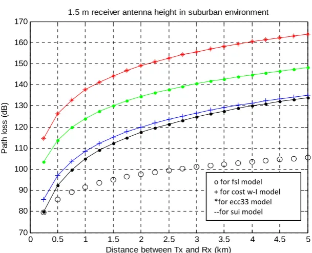
The following graphs plot for the 1.5m Mobile receiver antenna height, 40m Base station antenna height and frequency is 900MHz. The figure I shows graph between the path loss and distance from transmitter to receiver for Urban Environment. Similarly figure 2 and figure 3 graphs shows for Rural and Suburban environment. Figure 1 : Path loss at Urban aera
0 0.5 1 1.5 2 2.5 3 3.5 4 4.5 5
70 80 90 100 110 120 130 140 150 160 170
Distance between Tx and Rx (km)
Pa
th
l
o
s
s
(
d
B)
1.5 m receiver antenna height in urban environment
o for fsl model + for cost w-I model *for ecc33 model
Figure 2: Path Loss at Rural area
Figure 3: Path loss at suburban area
5. Conclusion:
In this paper we compare different types of propagation model with their path loss equation and graphs. Some of them model are used in urban, suburban area but some are in rural areas. For example Hata Model is better in suburban areas and the ECC-33 Model in urban areas.
0 0.5 1 1.5 2 2.5 3 3.5 4 4.5 5
70 80 90 100 110 120 130 140 150 160
Distance between Tx and Rx (km)
Pa
th
l
o
s
s
(
d
B)
1.5 m receiver antenna height in rural environment
0 0.5 1 1.5 2 2.5 3 3.5 4 4.5 5
70 80 90 100 110 120 130 140 150 160 170
Distance between Tx and Rx (km)
Pa
th
lo
s
s
(
d
B)
1.5 m receiver antenna height in suburban environment
0 for fsl model + for cost w-I model --for cost hata model *for sui model
References
[1] H.R.Aderson, “Fixed Broadband Wireless system Design” John Wiley & co 2003.
[2] Cruzl, R.M.S., F.C.Da Costal, P.F.Bragal, G. Fontgalland , M.A.B. Demeloand R.R.M. Do Valle “A comparision between theoretical propagation models and measurement data to distinguish urban, suburban and open aeras in Jodo Pessoa,Brazil” IEEE Microwave and Optoelectronics, 287-291,July 2005.
[3] K.Ayyappan, P.Dananjayan, “Propagation model for highway in mobile communication system” may 2007
[4] [4] H.K.Sharma, S.Sahu, S.Sharma, “ Enhanced Cost231 W.I. Propagation Model in Wireless Network” International Journal of Computer Applications, volume 19- No 6, April 20011.
[5] T.S.Rappaport, “Wireless Communications”, Pearson Education, pp.150-154, Second Edition.
[6] Abhayawardhana, V.S.,et al.,2003, “comparison of Empirical propagation Path loss Model for Fixed Wireless Access Systems”. Project funded by Ofcom, UK
[7] V. Erceg, K. V. S. Hari, et al., “Channel models for fixed wireless applications,” tech. rep., IEEE 802.16 Broadband Wireless Access Working b Group, January 2001.
[8] V. Erceg, L.J.Greenstein, et al., “An Empirically Path loss model for Wireless channels in suburban environments” IEEE Journal on selected areas of Communications, vol. 17,pp.1205-1211, July1999.
[9] The Egli Model is described in “Radio Propagation above 40MC Over Irregular Terrain, (Proceeding of the IRE, vol.45, Oct. 1957, pp1383-1391).
[10] P.K.Sharma, et. Al./ International journal of Engineering Science and Technology,Vol.2(6), 2010, 2008-2013.
[11] Armoogum.V, Soyjaudah.K.M.S, FogartyT.andMohamudallyN.,”Comparative study of Path loss using existing models for Digital Television Broadcasting for Summer, Mauritius Vol. 4, pp 34-38,May Season in the north of Mauritius”, Proceeding of Third Advanced IEEE International Conference on Telecommunication 2007.
[12] M. Hata, “Empirical formula for propagation loss in land mobile radio services,” IEEE Transactions on Vehicular Technology, vol. vol. VT-29, pp. 317–325, September 1981.
Mrs. Pooja Prajesh was born on 30th June 1978 in Roorkee, Uttrakhand (India). She received her M.Tech.degree in Digital Communication from Uttrakhand Technical University (U.K.), India. She is a Associate Member of the AMIETE. She has published several Research papers in national and international journals/conferences. She is presently research scholar in Uttarakhand Technical University, Dehradun (India) . Her present research interest is in Wireless Communication.