ANALYSIS OF ACCELERATED LIFE TESTING USING LOG-LOGISTIC GEOMETRIC PROCESS MODEL IN CASE OF CENSORED DATA

ANALYSIS OF

ACCELERATED LIFE

TESTING USING LOG-LOGISTIC

GEOMETRIC PROCESS MODEL IN

CASE OF CENSORED DATA

S. SAXENA

Department of Statistics & Operations Research, Aligarh Muslim University, Aligarh, Uttar Pradesh, India

[email protected] MUSTAFA KAMAL

Department of Statistics & Operations Research, Aligarh Muslim University, Aligarh, Uttar Pradesh, India

[email protected] SHAZIA ZARRIN

Department of Statistics & Operations Research, Aligarh Muslim University, Aligarh, Uttar Pradesh, India

[email protected] ARIF-UL-ISLAM

Department of Statistics & Operations Research, Aligarh Muslim University, Aligarh, Uttar Pradesh, India

[email protected] Abstract:

Geometric process model has been used in a variety of situations such as the determination of the optimal replacement policy and the optimal inspection-repair replacement policy for standby systems, and the analysis of data with trends. This study deals with the analysis of accelerated life testing for Log-Logistic distribution using geometric process model. The case of type-I censoring is considered in this study. It is assumed that the lifetimes under increasing stress levels form a geometric process. The maximum likelihood estimates of the parameters and their confidence intervals using the asymptotic method are derived. The performance of the estimators is evaluated by a simulation study with different pre-fixed parameters.

Keywords: Geometric process; Maximum Likelihood Estimator; Fisher Information Matrix; 1. Introduction

Traditional life tests are conducted to evaluate product reliability. In general, certain number of samples is tested under normal operating conditions to infer the parameters of the life distribution for the product. Because most products have high reliability these days, traditional life tests will have long durations which renders them of no practical use. One way to overcome this problem is by using accelerated life tests (ALTs) in which the failures are induced in the samples by subjecting them to operating conditions that are more severe than normal ones. Interested readers can refer to [Meeker and Escobar (1998)] and Nelson [(1990)].

Accelerated life tests are mainly based on three types of stress: constant stress, step stress and linearly increasing stress. The constant stress loading is a time-independent test setting and has several advantages over the time-dependent stress loadings. For example, it is assumed that most products operate at a constant stress under normal use. Therefore, a constant stress test seems to mimic the actual use. Also, it is comparatively easy to run and to quantify a constant stress test. In the present study, we are concerned only with the application of constant stress in accelerated life testing.

1.1 Definition:

A stochastic process {X_n,n1,2,...}is a geometric process (GP), if there exists a real





0

such that ,...}

2 , 1 ,

{



n1X_n n forms a renewal process (RP). The number



is called the ratio of the GP.

A considerable amount of work has been done to present and improve the GP. The GP has been introduced as a simple monotone process by [Lam (1988a), (1988b)]. Thereafter he applied it to the maintenance problem of a one-component system [Lam (2003)]. The GP was also used in the study of the maintenance problem for a two-component system; see [Lam (1995)], [Lam and Zhang (1996)], and [Zhang (1999)]. Furthermore, [Lam (1992a)], [Lam and Chan (1998)], and [Lam et al. (2004)] applied the GPM to the analysis of data from a series of events. [Zhang et al. (2002)] also studied a monotone process model for the maintenance problem of a multistate system.

The usefulness of the GP and its relatives in reliability and scheduling applications depends upon the first moment being finite. Many of the equations which result from such optimization problems contain terms involving this moment explicitly. Furthermore, numerical methods are usually required to calculate approximations for this moment; clearly, one should not attempt such a calculation if the moment does not exist.

In this paper, the GP model is extended for the analysis of accelerated life testing with log-logistic distribution under constant stress with type-I censoring. Statistical inference of the parameters are made and examined through a simulation study. It is reasonable to believe that in an accelerated life testing, lifetimes of products are stochastically decreasing with respect to increasing stress levels. Therefore, the geometric process model is a natural approach to study such problems.

2. The Model

2.1. The geometric process

Let us define the geometric process, see [Lam (1991, 2007)]. Suppose that X₁,X₂,...,X_nis a sequence of random variables. If there exists





0

such that {



n1X_n,n1,2,...}forms a renewal process (RP) with a constant mean



, then X₁,X₂,...,X_n is called a geometric process (GP) and the real number



is called the ratio of the GP. It can easily be noted that a GP is stochastically increasing for

0







1

and stochastically decreasing in case of





1

. GP model can identify trend effects by two parameters: the mean



of the underlying RP and the ratio



which measures the direction and strength of a trend. With the inherent geometric structure, forecast using the GPM is simple and straightforward.

2.1.1. Mean and variance of a geometric process:

It can be shown that if {X_n,n1,2,...} is a GP and the probability density function (pdf) of X₁ is f(x) with mean  and variance



2 then the pdf of X_n will be

( ), 1,2,...

1

1  _

 _f n _{x n}

n

_



1

/ )

(X_n  n

E





And Var(X_n)



2/



2(n1). Thus

 

,

and



2 are three important parameters of a GP.

2.2. The log-logistic distribution

The log-logistic distribution is a continuous probability distribution for a non-negative random variable. It is used in survival analysis as a parametric model for events whose rate increases initially and decreases later, for example mortality from cancer following diagnosis or treatment.

The probability density function (pdf) of a two parameter Log-Logistic distribution is given by





    

  

 

0 0

0 ,

] ) ( 1 [ ,

1 2

x x x

x x

f

  









where



0 is the shape parameter and





0

_{is the scale parameter and is also the median of the}

There are several different parameterizations of the distribution in use. The one shown here gives reasonably interpretable parameters and a simple form for the cumulative distribution function (cdf). Hence, the cdf for the Log-Logistic distribution is





    

  



0 0

0 ,

) ( 1

1

,

x x x

x

F









The log-logistic distribution provides one parametric model for survival analysis. Unlike the more commonly used Weibull distribution, it can have a non-monotonic hazard function. The fact that the CDF can be written in closed form is particularly useful for analysis of survival data with censoring, [Bennett (1983)]. The log-logistic distribution can be used as the basis of an accelerated failure time model by allowing  to differ between groups, or more generally by introducing covariates that affect but not



by modeling log



as a linear function of the covariates, [Collett (2003)].

The survival function of the Log-Logistic distribution takes the following form 0 ,

) ( 1

) ( ) , |

( 



 x

x x x

S _











The failure rate (or hazard rate) for the Log-Logistic distribution is given by 0 ,

) ( 1

1 )

, |

( 



 x

x x x

h _









2.3. Assumptions

The geometric model for ALT is based on the following assumptions:

(1) Suppose that an ALT underz_k, k 1,2,...,s, arithmetically increasing stress levels is performed. A random sample of N_i, i1,2,...,n, identical items is placed under each stress level and start to operate at the same time. Whenever an item fails, it is removed from the test and its observed failure time x_ki is recorded.

(2) At any constant stress level, the product lifetime has a two parameter Log-Logistic distribution.

(3) Let the sequence of random variablesX₀,X₁,X₂,...,X_s, denote the lifetimes under each stress level, where X₀denotes item’s lifetime under the design stress. We assume



X_k,k 1,2,...,s



is a GP with ratio





0

.

Based on the definition given in subsection 2.1, if density function ofX₀isf (x), then the pdf of X_kwill be given by

s k

x

f k

k

, , 2 , 1 , 0 ,

)

(



 



Therefore the pdf of a product lifetime at the kth stress level is

2 1

] ) ( 1 [

) ( )

, , |

( _{ }

 

















x x x

f

k k k

xk  _



2.4. Maximum Likelihood Estimation

For Type I censoring scheme, the test at each stress level terminates at timet. An item’s exact failure time is observed only if its lifetime isx_ki t. It is assumed that at the kth stress level r_k(n) failures are observed before the test is suspended. Correspondingly, (nr_k)units survive the entire test without failing. The observed ordered failure times under the kth stress level can be written as _{(1) (2) ( )}

k

r k k

k x x

x   . Here, t





k k k r n X i X r i k

k f x S t

r n n L            



( ) ( ) ! ) ( ! ) , , ( _{( )} 1







(1)

where, S_Xk(t)is the probability that an item is censored at time tand

 





) ( 1 ) ( ) ( t t t S k k

Xk  _ (2) Using eq. (2), the likelihood function for one of the stress levels corresponding to eq. (1) for obtaining the ML estimates for_,  and



is given by





, ) ( 1 ) ( ) ( 1 ) ( ! ) ( ! ) , , ( ) ( 1

1 ₍₎ 2

) ( k r n k t t x x r n n L _k k r

i k _{k i}

i k k k i                      

_

    



























x x x t

t t x x r n n k k r n k k k r k k k k k r i i k k i k k r k r                           



1 2 (1) (2) ( )

) ( ) ( 0 , ) ( 1 ) ( ) ( 1 ! ) ( ) ( ! ) ( 1              (3)

It follows that the likelihood function of observed data in a total s stress levels is:

s

k L L L

L (



,



,



) ₁ ₂





, ) ( 1 ) ( ) ( 1 ! ) ( ) ( ! ) ( 1 1 2 ) ( ) ( 1 k r n k k k t t x x r n n k k r i i k k i k k r k r s k                      

_

_

     

















x x x t k s

k

r k k

k      

 ;1

0 _{(1) (2)}  _{( )} (4) The log-likelihood function corresponding (4) takes the form





           s k r i i k k k k k k x k r r r r n n L l 1 1 ) ( log ) 1 ( log log log ! ) ( ! log ) , , (

log























          

_

_

  k k r i k k r i i k

k_{x n r k t t}

1 1

)

( ) ) ( )log log log log(1 ( ) )

( 1 log(

2











 (5)

The first order derivatives of logL(



,



,



) are given by

                        







     k k r i r i k k k i k k i k k k s k t t k k r n x x k r k l 1 1 1 ) ( ) ( 1

1 (1 ( ) )

) ( ) ( ) ) ( 1 ( ) ( 2 _     





















(6)









                              s k r i r i k k k k i k k i k k i k k r i i k k k

k k k k

t t t r n x x x x r r l

1 1 () 1

) ( ) ( 1 ) ( ) ) ( 1 ( ) log( ) ( ) ( ) ) ( 1 ( ) log( ) ( 2 log log _             (7)







                              s k r i r i k k k i k k i k k

k k k

t t r n x x r l

1 1 1

1 ) ( ) ( 1 ) ) ( 1 ( ) ( 1 ) ( ) ) ( 1 ( ) ( 2 _     





















(8)

The equations (6), (7) and (8) are quite complex in form to be solved. So, the Newton-Raphson method is used to solve these equations simultaneously to obtain



ˆ



ˆ and



ˆ

.

           33 32 31 23 22 21 13 12 11 ˆ ˆ ˆ ˆ ˆ ˆ ˆ ˆ ˆ I I I I I I I I I F where









                    

_

_

   k r

i k k i

i k k i k k k s k x x k x k k r l I

1 () 2

) ( ) ( 2 2 1 2 2 11 ) ) ( 1 ( ) ( 1 ) ( 2 ˆ    



























                  

_

  k r i k k k k t t k t k k r n 1 2 2

2 _{(1 ( ) )}

) ( 1 ) ( ) ( _   



















                                     s k r i r i k k k k i k k i k k i k k

k k k

t t t r n x x x r l I

1 1 1 2

2 2 ) ( 2 ) ( ) ( 2 2 2 22 ) ) ( 1 ( ) (log ) ( ) ( ) ) ( 1 ( ) (log ) ( 2 ˆ    

























                        s k r

i k k i

i k k i k k k k x x x r l I

1 1 () 2

) ( ) ( 2 2 2 2 33 ) ) ( 1 ( ) ( ) 1 ( ) ( 2 ˆ    

















          _{  }   

_

  k r i k k k

k _{t t}

t r n 1 2 2

2 ( ) {( 1) ( )

1 ) ) ( 1 ( ) ( _{  } 

_















                         s k r

i k k i

i k k i k k i k k k k x x x x k kr I l I

1 1 () 2

) ( ) ( ) ( 21 2 12 ) ) ( 1 ( ) log( ) ( 1 { ) ( 2 ˆ ˆ   



















        

_

 k r i k k k k k t t t t r n k

1 (1 ( ) )2

) log( ) ( 1 { ) ( ) (   



















                                  s k r i k k i k r

i k k i

k k k

t t r n x x k I l I

1 1 2

1

) (

1 () 2

1 ) 1 ( 13 2 31 ) ) ( 1 ( ) ( ) ) ( 1 ( 2 ˆ ˆ       



















                         s k r

i k _{k i}

i k k i k k i k k k k x x x x r I l I

1 1 ₍₎ 2

) ( ) ( ) ( 32 2 23 ) ) ( 1 ( ) log( ) ( 1 { ) ( 2 ˆ ˆ   



















        

_

 k r i k k k k k t t t t r n

1 (1 ( ) )2

) log( ) ( 1 { ) ( ) (   













Now, the variance covariance matrix can be written as

                        ) ˆ ( ) ˆ ˆ ( ) ˆ ˆ ( ) ˆ ˆ ( ) ˆ ( ) ˆ ˆ ( ) ˆ ˆ ( ) ˆ ˆ ( ) ˆ ( ˆ ˆ ˆ ˆ ˆ ˆ ˆ ˆ ˆ 1 33 32 31 23 22 21 13 12 11































AVar ACov ACov ACov AVar ACov ACov ACov AVar I I I I I I I I I

The

100

(

1





)%

asymptotic confidence interval for



,



and



are then given respectively as

          ) ˆ ( ˆ 2 1





Z _ AVar ,

          (ˆ) ˆ 2 1





Z _ AVar and

          (ˆ) ˆ 2 1



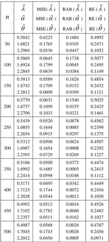
5. Simulation Study

To assess the performance of the method described in present study, a number of data sets with sample sizes

n=50,100,...,500 are generated from Log-logistic distribution. The values for true parameters and stress levels are chosen to be



0.50,



2.20



1.70ands2or 4 and the Newton-Raphson iteration procedure is applied. For different given samples and stress levels, the Maximum Likelihood (ML) estimates, Mean squared errors (MSEs), absolute relative biases (RBias), Relative Error (RE), and the 95% and 99% asymptotic confidence intervals for



,



and



are obtained by using the present GPM. The results of the estimates for



,



and



based on 1000 replications are summarized in Table 1 and 2 while the confidence intervals are shown in Table 3 and 4 respectively.

Table 1: Simulation Study Results with



0.50_,



2.20



1.70and s2

n



ˆ



ˆ



ˆ

MSE(



ˆ

) MSE (



ˆ) MSE (



ˆ)

RAB (



ˆ

) RAB (



ˆ) RAB (



ˆ)

RE (



ˆ

) RE (



ˆ) RE (



ˆ) 50

0.5842 1.6821 2.2984

0.6223 0.1765 0.0536

0.1684 0.0105 0.0447

0.4992 0.2471 0.1052

100 0.5869 1.6924 2.2845

0.0645 0.1799 0.0639

0.1738 0.0045 0.0384

0.5077 0.2495 0.1149

150 0.5813 1.6742 2.2812

0.0589 0.1709 0.0608

0.1626 0.0152 0.0369

0.4854 0.2432 0.1121

200 0.5770 1.6737 2.2706

0.0631 0.1699 0.1033

0.1540 0.0155 0.0321

0.5025 0.2425 0.1461

250 0.5439 1.6855 2.2654

0.0520 0.1644 0.0915

0.0878 0.0085 0.0297

0.4562 0.2399 0.1375

300 0.5312 1.6987 2.2593

0.0508 0.1654 0.0729

0.0624 0.0008 0.0269

0.4507 0.2392 0.1227

350 0.5186 1.6992 2.2414

0.0500 0.1685 0.0598

0.0372 0.0005 0.0188

0.4474 0.2415 0.1112

400 0.5171 1.7123 2.2028

0.0495 0.1744 0.0544

0.0342 0.0072 0.0012

0.4449 0.2456 0.1058

450 0.4992 1.7102 2.2357

0.0512 0.1782 0.0511

0.0016 0.0060 0.0162

0.4526 0.2483 0.1027

500 0.4987 1.7045 2.2012

0.0568 0.1743 0.0456

0.0026 0.0026 0.0005

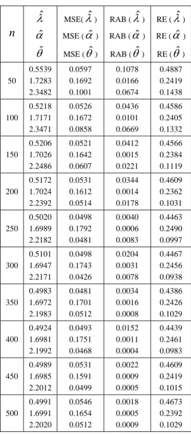
Table 2: Simulation Study Results with



0.50_,



2.20



1.70and s4

n



ˆ



ˆ



ˆ

MSE(



ˆ

) MSE (



ˆ) MSE (



ˆ)

RAB (



ˆ

) RAB (



ˆ) RAB (



ˆ)

RE (



ˆ

) RE (



ˆ) RE (



ˆ) 50

0.5539 1.7283 2.3482

0.0597 0.1692 0.1001

0.1078 0.0166 0.0674

0.4887 0.2419 0.1438

100 0.5218 1.7171 2.3471

0.0526 0.1672 0.0858

0.0436 0.0101 0.0669

0.4586 0.2405 0.1332

150 0.5206 1.7026 2.2486

0.0521 0.1642 0.0607

0.0412 0.0015 0.0221

0.4566 0.2384 0.1119

200 0.5172 1.7024 2.2392

0.0531 0.1612 0.0514

0.0344 0.0014 0.0178

0.4609 0.2362 0.1031

250 0.5020 1.6989 2.2182

0.0498 0.1792 0.0481

0.0040 0.0006 0.0083

0.4463 0.2490 0.0997

300 0.5101 1.6947 2.2171

0.0498 0.1743 0.0426

0.0204 0.0031 0.0078

0.4467 0.2456 0.0938

350 0.4983 1.6972 2.1983

0.0481 0.1701 0.0512

0.0034 0.0016 0.0008

0.4386 0.2426 0.1029

400 0.4924 1.6981 2.1992

0.0493 0.1751 0.0468

0.0152 0.0011 0.0004

0.4439 0.2461 0.0983

450 0.4989 1.6985 2.2012

0.0531 0.1591 0.0499

0.0022 0.0009 0.0005

0.4609 0.2419 0.1015

500 0.4991 1.6991 2.2020

0.0546 0.1654 0.0512

0.0018 0.0005 0.0009

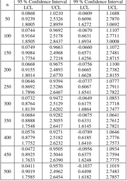
Table 3: Confidence Intervals using



0.50_,



2.20



1.70and s2

n

95 % Confidence Interval 99 % Confidence Interval

LCL UCL LCL UCL

50

0.1237 0.8594 1.8877

1.0447 2.5048 2.7091

-0.0219 0.5991 1.7578

1.1904 2.7651 2.8389

100

0.1194 0.8619 1.8174

1.0544 2.5235 2.7516

-0.0285 0.5984 1.6696

1.2023 2.7864 2.8994

150

0.1331 0.8656 1.8249

1.0295 2.4828 2.7375

-0.0087 0.6098 1.6806

1.1713 2.7386 2.8818

200

0.1082 0.8675 1.6561

1.0458 2.4799 2.8851

-0.0400 0.6124 1.4617

1.1940 2.7349 3.0795

250

0.1052 0.8865 1.6866

0.9826 2.4845 2.8442

-0.0336 0.6337 1.5035

1.1214 2.7373 3.0272

300

0.0938 0.9016 1.7429

0.9686 2.4958 2.7756

-0.0446 0.6494 1.5796

1.1069 2.7479 2.9389

350

0.0816 0.8946 1.7689

0.9556 2.5038 2.7138

-0.0565 0.6401 1.6195

1.0938 2.7582 2.8633

400

0.0824 0.8942 1.7465

0.9518 2.5304 2.6591

-0.0552 0.6355 1.6022

1.0894 2.7891 2.8034

450

0.0557 0.8830 1.7983

0.9427 2.5374 2.6731

-0.0846 0.6214 1.6599

1.0829 2.7990 2.8115

500

0.0316 0.8862 1.7827

0.9658 2.5228 2.6197

-0.1162 0.6274 1.6502

1.1136 2.7816 2.7521

Table 4: Confidence Intervals using



0.50_,



2.20



1.70and s4 n 95 % Confidence Interval 99 % Confidence Interval

LCL UCL LCL UCL

50

0.0868 0.9239 1.8005

1.0210 2.5326 2.8959

-0.0609 0.6696 1.6272

1.1688 2.7870 3.0692

100

0.0744 0.9164 1.8505

0.9692 2.5178 2.8437

-0.0670 0.6631 1.6934

1.1107 2.7711 3.0008

150

0.0749 0.9084 1.7754

0.9663 2.4968 2.7218

-0.0660 0.6571 1.6256

1.1072 2.7481 2.8715

200

0.0668 0.9155 1.8014

0.9675 2.4893 2.6770

-0.0756 0.6665 1.6628

1.1100 2.7382 2.8155

250

0.0646 0.8692 1.7896

0.9394 2.5286 2.6467

-0.0737 0.6067 1.6541

1.0777 2.7911 2.7822

300

0.0732 0.8764 1.8139

0.9472 2.5129 2.6202

-0.0649 0.6175 1.6864

1.0853 2.7718 2.7477

350

0.0684 0.8888 1.7548

0.9282 2.5055 2.6417

-0.0675 0.6331 1.6145

1.0641 2.7612 2.7821

400

0.0576 0.8779 1.7752

0.9271 2.5182 2.6232

-0.0789 0.6185 1.6410

1.0646 2.7776 2.7573

450

0.0472 0.8925 1.7633

0.9505 2.5044 2.6390

-0.0956 0.6375 1.6248

1.0934 2.7594 2.7775

500

0.0411 0.9019 1.7585

0.9570 2.4962 2.6454

-0.1037 0.6498 1.6182

From the results in the above tables the following observations can be made on the performance of parameter estimation of log-logistic distribution using GPM

(1) For the first set of values the ML estimators have good statistical properties (as the parameter estimates are close to their true values) than the second.

(2) As the sample size increase the estimates have smaller MSE and RE. This indicates that the ML estimates provide asymptotically normally distributed and consistent estimator for the parameters. (3) The asymptotic variances of the estimators are decreasing when the sample size increasing. (4) As the sample size increases, the width of asymptotic confidence interval decreases. 6. Discussion and Conclusion

This study deals with use of GPM in the analysis of constant stress ALT plan for log-logistic distribution with type-I censoring plan. The MLEs, MSEs, RBias, and RE of the model parameters were obtained. Based on the asymptotic normality, the 95% and 99% asymptotic confidence intervals of the model parameters were also obtained. It is observed that the estimates obtained in the simulation study are very close to the true values of the parameters and are also quite well with relatively small mean squared errors. In the whole study, the parameters are estimated for different cases and it is found that as the sample size increases, the MSE gets smaller. It implies that a larger sample size results in a better sample approximation. Hence, it can be said that the proposed GPM can be used in the analysis of accelerated life testing.

References

[1] Bennett, S. (1983): Log-Logistic regression models for survival data, Journal of the Royal Statistical Society, Series C (Applied Statistics), 32, 2, pp. 165–171.

[2] Collett, D. (2003): Modeling survival data in medical research (2nd ed.), CRC press.

[3] Lam, Y. (1988a): A note on the optimal replacement problem, Advances in Applied Probability, 20, pp. 479-482. [4] Lam, Y. (1988b): Geometric processes and replacement problem, Acta Mathematicae Applicatae Sinica, 4, pp. 366-377. [5] Lam, Y. (1992a): Nonparametric inference for geometric processes, Commun. Statist. Theory Meth, 21, pp. 2083-2105.

[6] Lam, Y. (1995): Calculating the rate of occurrence of failures for continuous-time markov chains with application to a two-component parallel system, J. Operat. Res. Soc., 46, pp. 528-536.

[7] Lam, Y. and Chan, S. K. (1998): Statistical inference for geometric processes with lognormal distribution, Computational Statistics and Data Analysis, 27, pp. 99-112.

[8] Lam, Y. and Zhang, Y. L. (1996): Analysis of a two-component series system with a geometric process model, Naval Res. Logistics, 43, pp. 491-502.

[9] Lam, Y., Zhu, L. X., Chan, S. K. and Liu, Q. (2004): Analysis of data from a series of events by a geometric process model, Acta Math. Appl. Sinica, 20, pp. 263-282.

[10] Meeker, W. Q. and Escobar, L. A. (1998): Statistical methods for reliability data, New York, John Wiley & Sons. [11] Nelson, W. (1990): Accelerated Testing: Statistical Models, Test Plans, and Data Analyses, New York, John Wiley & Sons. [12] Y. Lam (1991): An optimal repairable replacement model for deteriorating systems, J. Appl. Prob., 28, pp. 843-851. [13] Y. Lam (2007): Geometric process and its applications, World Scientific Publishing.

[14] Zhang, Y. L. (1999): An optimal geometric process model for a cold standby repairable system, Reliab. Eng. Systems Safety, 63, pp. 107-110.