https://doi.org/10.5194/amt-12-4241-2019 © Author(s) 2019. This work is distributed under the Creative Commons Attribution 4.0 License.
Analysis algorithm for sky type and ice halo recognition
in all-sky images
Sylke Boyd, Stephen Sorenson, Shelby Richard, Michelle King, and Morton Greenslit
Division for Science and Mathematics, University of Minnesota Morris, 500 E 4th Street, Morris, MN, USA Correspondence:Sylke Boyd ([email protected])
Received: 15 November 2018 – Discussion started: 7 January 2019
Revised: 14 June 2019 – Accepted: 10 July 2019 – Published: 6 August 2019
Abstract.Halo displays, in particular the 22◦halo, have been captured in long time series of images obtained from total sky imagers (TSIs) at various Atmospheric Radiation Mea-surement (ARM) sites. Halo displays form if smooth-faced hexagonal ice crystals are present in the optical path. We de-scribe an image analysis algorithm for long time series of TSI images which scores images with respect to the pres-ence of 22◦halos. Each image is assigned an ice halo score (IHS) for 22◦halos, as well as a photographic sky type (PST), which differentiates cirrostratus (PST-CS), partially cloudy (PST-PCL), cloudy (PST-CLD), or clear (PST-CLR) within a near-solar image analysis area. The color-resolved radial brightness behavior of the near-solar region is used to de-fine the discriminant properties used to classify photographic sky type and assign an ice halo score. The scoring is based on the tools of multivariate Gaussian analysis applied to a standardized sun-centered image produced from the raw TSI image, following a series of calibrations, rotation, and co-ordinate transformation. The algorithm is trained based on a training set for each class of images. We present test re-sults on halo observations and photographic sky type for the first 4 months of the year 2018, for TSI images obtained at the Southern Great Plains (SGP) ARM site. A detailed comparison of visual and algorithm scores for the month of March 2018 shows that the algorithm is about 90 % reliable in discriminating the four photographic sky types and iden-tifies 86 % of all visual halos correctly. Numerous instances of halo appearances were identified for the period January through April 2018, with persistence times between 5 and 220 min. Varying by month, we found that between 9 % and 22 % of cirrostratus skies exhibited a full or partial 22◦halo.
1 Introduction
al., 2007; Schwartz et al., 2014). Cirrostratus clouds, lacking sharp outlines, pose a challenge to this approach (Schwartz et al., 2014). The uncertainty about the role of cirrus in the global energy balance has been attributed to limited obser-vational data concerning their temporal and spatial distribu-tion, as well as their microphysics (Waliser et al., 2009). Cir-roform clouds, at altitudes between 5000 and 12 000 m, are effective LW absorbers. Cloud particle sizes can range from a few microns to even centimeter sizes (Cziczo and Froyd, 2014; Heymsfield et al., 2013). Methods to probe cirrus cloud particles directly involve aircraft sampling (Heymsfield et al., 2013) and mountainside observations (Hammer et al., 2015). Ground- and satellite-based indirect radar and lidar measure-ments (Hammer et al., 2015; Hong et al., 2016; Tian et al., 2010) give reliable data on altitudes, optical depths, and par-ticle phase. Even combined, these methods leave gaps in the data for spatial and temporal composition of ice clouds. The analysis of halo displays as captured by long-term total sky imagers may provide further insight and allow one to close some of the gaps.
Optical scattering behavior is influenced by the types of ice particles, which may be present in very many forms, in-cluding crystalline hexagonal habits in the form of plates, pencils and prisms, hollow columns, bullets and bullet rosettes, and amorphous ice pellets, fragments, rimed crys-tals, and others (Bailey and Hallett, 2009; Baran, 2009; Yang et al., 2015). Only ice particles with a simple crystal habit and smooth surfaces can lead to halo displays (Um and Mc-Farquhar, 2015; van Diedenhoven, 2014). Usually, this will be the hexagonal prism habit, which we can find in plates, columns, bullet rosettes, pencil crystals, etc. If no preferred orientation exists, a clear telltale sign for their presence is the 22◦ halo around a light source in the sky, usually sun or moon. More symmetry in the particle orientations will add additional halo display features such as parhelia, upper tangent arc, circumscribed halo, and others (Greenler, 1980; Tape and Moilanen, 2006). As shown in theoretical stud-ies (van Diedenhoven, 2014; Yang et al., 2015), halos form in particular if the ice crystals exhibit smooth surfaces. In that case, the forward-scattered intensity is much more pro-nounced as in cases of rough surfaces, even if a crystal habit is present. If many of the ice particles are amorphous in na-ture, or did not form under conditions of crystal growth – for example by freezing from supercooled droplets, or by riming – the forward scattering pattern will be weaker and similar to what we see for liquid droplets: a white scatter-ing disk surroundscatter-ing the sun, but no halo. In turn, roughness and asymmetry of ice crystals influence the magnitude of backscattered solar radiation, thus influencing the radiative effect of cirrus clouds (van Diedenhoven, 2016). If the parti-cles in the cirroform cloud are very small, e.g., a few microns (Sassen, 1991), diffraction will lead to a corona. We believe that a systematic observation of the optical scattering proper-ties adds information to our data on cirrus microphysics and cirrus radiative properties. The authors observed the sky at
the University of Minnesota Morris, using an all-sky camera, through a 5-month period in 2015, and found an abundance of halo features.
There are a few studies pursuing a similar line of inquiry (Forster et al., 2017; Sassen et al., 2003). The study by Sassen et al. (2003) showed a prevalence of the 22◦halo, full in 6 % and partial in 37.3 % of cirrus periods, based on a 10-year photographic and lidar record of midlatitude cirrus clouds, also providing data on parhelia, upper tangent arcs, and other halo display features, as well as coronas. The photographic record was taken in Utah and based on 20 min observation intervals; cirrus identification was supported by lidar. The authors found an interesting variability in halo displays, re-lated to geographical air mass origin, and suggest that optical displays may serve as tracers of the cloud microphysics in-volved. Forster et al. (2017) used a sun-tracking camera sys-tem to observe halo display details over the course of several months in Munich, Germany, and a multiweek campaign in the Netherlands in November 2014. A carefully calibrated camera system provided high-resolution images, for which a halo detection algorithm was presented, based on a deci-sion tree and random forest classifiers. Ceilometer data and cloud temperature measurements from radiosonde measure-ments were used to identify cirrus clouds. The authors report 25 % of all cirrus clouds also produced halo displays, in par-ticular in the sky segments located above the sun. The frac-tion of smooth crystals necessary for halo display appearance is at a minimum 10 % for columns, and 40 % for plates, based on an analysis of scattering phase functions for single scatter-ing events (van Diedenhoven, 2014). While this establishes a lower boundary, it is correct to say that the observability of a halo display allows one to conclude that smooth crystalline ice particles are present and single scattering events domi-nate. The consideration of the percentage of cirrus clouds that display optical halo features allows therefore, upon further study, inferences about the microphysical properties of the cloud. This raises interest in examining existing long-term records of sky images.
discrimi-nate them from clouds and or 22◦halos. If present they would be classified by this algorithm as part of a 22◦halo. Coronas are obscured by the shadow strip and often also by overexpo-sure in the near-solar area of the image. The algorithm offers an efficient method of finding 22◦ halo incidences, full or partial. Since ARM sites also have collected records of li-dar and radiometric data, the TSI halo algorithm is intended to be compared to other instrumental records from the same locations and times. This will be addressed in future work.
Section 1 describes the TSI data used in this work. Sec-tion 2 presents the details of the image analysis algorithm, including subsections on algorithm goals, image preparation, and sky type and halo scoring. Section 3 applies the algo-rithm to the TSI data record of the first 4 months of 2018 and examines the effectiveness and types of data available for this interval. Summary and outlook are given in Sect. 4.
2 TSI images
Images used in this paper were obtained from Atmospheric Research Measurement (ARM) Climate Research Facilities in three different locations: Eastern North Atlantic (ENA) Graciosa Island, Azores, Portugal; North Slope of Alaska (NSA) Central Facility, Barrow, AK; and Southern Great Plains (SGP) Central Facility, Lamont, OK (ARM, 2000). The ranges and dates vary by location, as listed in Table 1. The images were taken with total sky imagers, which consist of a camera directed downward toward a convex mirror to view the whole sky from zenith to horizon. A sun-tracking shadow band is used to block the sun, which covers a strip of sky from zenith to horizon. Images were recorded every 30 s. The longest series was taken at the Southern Great Plains location, reaching back to July 2000. The images, in JPEG format, have been taken continuously during daytime. Aside from nighttime and polar night, there are some additional gaps in the data, perhaps due to instrument failure or other causes. Camera quality, exposure, mirror reflectance, image resolution, and image orientation varies over time as well as by location. For example, an image from SGP taken in 2018 has a size of 488 pixels by 640 pixels. The short dimension limits the radius of the view circle to at most 240 pixels. A pixel close to the center of the view circle corresponds to an angular sky section 2.8◦ wide and 0.24◦tall. At SGP, the solar position never reaches this point. Close to the hori-zon, 1-pixel averages a sky section that is 0.24◦ wide and 1.24◦tall. Best resolution is achieved at zenith angle 45◦, in which case every pixel represents a sky region of 0.33◦ by 0.33◦. The perspective distortion is largest for sky segments close to the horizon due to perspective distortions of the sky. We used a sampling of 80 images taken from across the TSI record and across all available years to initiate the training set (ARM, 2000). This included images visually classified from the images as photographic sky types CS, PCL, CLD, CLR, and halo-bearing. Descriptions of the PST are provided
in Table 2. The 80 sample images were used to develop the algorithm and define a suitable set of characteristic proper-ties for PST score (PSTS) and IHS. This set will be referred to as seed images since they also initialize the master table described below.
3 Algorithm
3.1 Goal and strategy
The algorithm aims to process very large numbers of images and return information about the presence of 22◦ halos, as well as the general sky conditions. The program is written in C++ and uses the OpenCV library for image process-ing. If given a list of image directories, the algorithm pro-ceeds to sequentially import, process, and score TSI images compared to training sets gleaned from representative im-ages for each scored class. We define four classes of photo-graphic sky types, listed in Table 2, and a halo class. The fac-tors that determine these choices are discussed in Sect. 2.3.1 and 2.3.3. The algorithm assigns a numeric photographic sky type score (PSTS) and a numeric ice halo score. For all im-age classes, sets of discriminant imim-age properties have been defined which differ between 10 distinct properties for PST classes and 31 distinct properties for the halo class.
Multivariate analysis is one of the standard methods in im-age analysis, applied in a wide variety of problems. Numer-ous text books provide introductions to this method in a the-oretical background (Harris, 1975; Gnanadesikan, 1977) as well as in an application-oriented manner (Alpaydin, 2014; Flury, 1988). A set ofNpdiscriminant properties of the
im-age is chosen, selected to be characteristic for a particular sky type or the presence of a halo. Let this set of properties be the observation vector
X= {xi} Np
i . (1)
For each class, a training set is created. The training set is a set ofNtobservation vectors for images that have been
visually assigned to the class. A training set defines an el-lipsoidal centroid in the property space ofX, centered at the mean observation vector
M= {µi} Np
i=1, (2)
µi=
1 Nt
XNt
k=1xik. (3)
The centroid’s extent is described by theNp×Np
covari-ance matrix
6=(X−M) (X−M)T =
σ11 σ12 . . . σ21 σ22 . . . . . . .
, (4)
with elements σij=
1 Nt
XNt
Table 1.TSI data set properties. Seed images for the algorithm were taken from all three locations. Data source: ARM (2000).
Location Dates and times (UTC) Image interval Resolution (pixels)
Southern Great Plains 2 Jul 2000 0:35:00 15 Aug 2011 01:17:30 30 s 288×352 36◦3601800N, 97◦290600W 15 Aug 2011 22:17:30 19 Apr 2018 01:02:00 30 s 480×640
North Slope of Alaska 25 Apr 2006 21:44:00 2 Nov 2010 21:31:00 30 s 288×352 71◦19022.800N, 156◦36032.400W 9 Mar 2011 01:08:30 11 Apr 2018 18:59:30 30 s 480×640
Eastern North Atlantic 1 Oct 2013 08:13:00 28 May 2018 21:04:00 30 s 480×640 39◦5029.7600N, 28◦1032.5200W
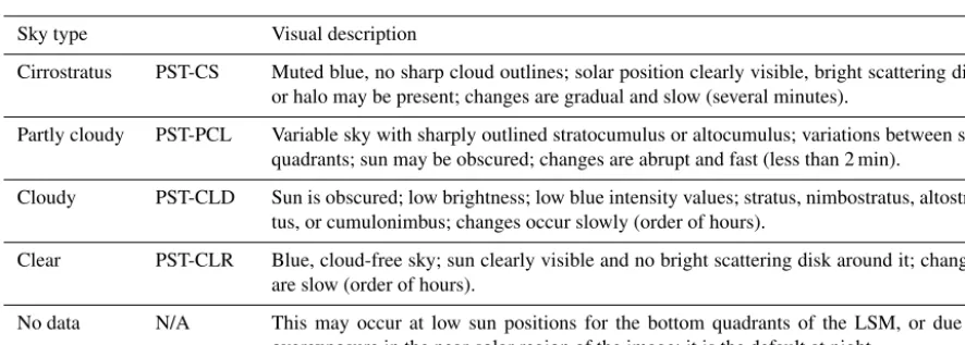
Table 2.Descriptions of the photographic sky types (PST).
Sky type Visual description
Cirrostratus PST-CS Muted blue, no sharp cloud outlines; solar position clearly visible, bright scattering disk or halo may be present; changes are gradual and slow (several minutes).
Partly cloudy PST-PCL Variable sky with sharply outlined stratocumulus or altocumulus; variations between sky quadrants; sun may be obscured; changes are abrupt and fast (less than 2 min).
Cloudy PST-CLD Sun is obscured; low brightness; low blue intensity values; stratus, nimbostratus, altostra-tus, or cumulonimbus; changes occur slowly (order of hours).
Clear PST-CLR Blue, cloud-free sky; sun clearly visible and no bright scattering disk around it; changes are slow (order of hours).
No data N/A This may occur at low sun positions for the bottom quadrants of the LSM, or due to overexposure in the near-solar region of the image; it is the default at night.
The observation vector of any further imageX0will then be referenced withM and6in the form of a multivariate nor-mal distribution:
F =C0exp
−1
2 X 0−MT
6−1 X0−M
, (6)
in which the quadratic form in the exponent is known as the square of the Mahalanobis distance in property space. The closer an image places to the centroid of a class, the higher its score Eq. (6) will be. The Mahalanobis distance is ex-pressed in units of standard deviations, eliminating the influ-ence of the units of the discriminant properties and the need for weights. It is interesting to note that the average Maha-lanobis distance for a class is equal to the number of discrim-inant properties. The prefactorC0in Eq. (6) is different for
the photographic sky type scores and the ice halo score since the dimensionality of the observation vectors for these two class types is different. It is chosen to place the values forF into a convenient number range. The valueF for each class of images is akin to a continuous numerical probability that the image is located close to the centroid of this particular class.
The algorithm is outlined in Fig. 1, together with the re-spective references to this text. Both M and6−1 are com-puted a priori from the training sets via Eqs. (2) and (4). In order to score a time series of property vectorsX, one only
needs to importM and6−1for each class once at the start
of the analysis run. The training sets for each class of images are started using the set of 80 images described in Sect. 1 and are expanded as needed. This allows one to continually train the algorithm toward improvement of scoring. This basic al-gorithm structure is used on a standardized local sky map, described in Sect. 2.2. The details of PSTS and IHS will be described separately below. The code and accessories can be accessed at a GitHub repository (Boyd et al., 2018).
3.2 Image preparations and local sky map (LSM)
con-Figure 1.Flow chart of the algorithm for the analysis of TSI images.
tains a solar 22◦halo, and the other one is a partly cloudy sky without any halo indications.
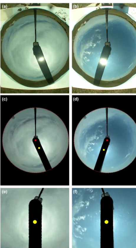
Step (1) is a color correction. Both original images in Fig. 2 have a slightly green tinge, which is typical for im-ages from the TSI at this location, in particular after an in-strument update in 2010. This is noticeable in particular if images are compared to earlier TSI data from the same loca-tion, and it can become a problem for the planned analysis, especially for the use of relative color values. Since the algo-rithm is intended for multiple TSI locations and records taken over a long time, including device changes, it is necessary to consider the fact that no two camera devices have exactly the same color response, even if of the same type (Ilie and Welch, 2005). The color calibration used in this algorithm is based on sampling of clear-sky color channels to define weighed scaling factors for a whole series of images. Every pixel in a TSI image exhibits a value between 0 and 255 for each of the three color channels blue (B), green (G), and red (R).
The color values represent the intensity of the color channel registered for the particular pixel, varying between 0 (no in-tensity) and 255 (brightest possible). In a discolored series, measurements of BGR were taken in clear-sky images (in-dexed PST-CLR), and a scaling factor and weight for each color channel were defined based on this information:
βB=1.00 βG=
Gref
GCLR
×BCLR
Bref βR=
Rref
RCLR
×BCLR
Bref
with(Bref, Gref, Rref)
=(180,120,85) . (7)
Figure 2. Two examples for image preparation. The left column develops an image from SGP 17 April 2018 17:45:00 UTC, and the right image was taken on SGP 3 April 2018 19:09:30 UTC.(a, b) Original image;(c, d)image after color correction, distortion removal, masking of horizon and equipment, and sun mark were applied;(e, f)final local sky map with sun at center and a width of about 80 LSM units.
and applying B0=
B+α βBB−B
G0=
G+α βGG−G
R0=B+α βRR−R
(8)
to each color channel and pixel, respectively, followed by a simple scaling to preserve the total brightness of the pixel I =
√
B2+G2+R2. For the series SGP 2018, these factors
wereβ=(0.9,0.78,1)andα=0.4. The coefficientα regu-lates the strength of the tinting such thatα=0 leads to no
tint, andα=1 produces an image of a single color. This tint-ing is minimal, and linear color behavior is a reasonable as-sumption.
Step (2) is a stretch-and-shift process that identifies the horizon circle. Occasionally, a slight misalignment of the camera and mirror axis leads to an elliptical appearance of the sky image. A calibration is necessary in such cases to stretch the visible horizon ellipse to a circular shape and to center the horizon circle as close to the zenith as possible. A north–south alignment correction may also have to be ap-plied. Both calibrations will ensure successful identification of the solar position in the next step. These calibrations be-come necessary if the TSI was not perfectly aligned in the field. They need to be readjusted after any disturbances oc-curred to the instrument, such as storms, snow, and instru-ment maintenance. Typically, this can be once every few months, or sometimes several times per month. It is impor-tant to check the calibrations regularly by sampling across the series whether the solar position was correctly identified after calibration. In addition, the horizon circle is placed at a zenith angle smaller than 90◦, often between 85 and 79◦, to eliminate the strong view distortion close to the horizon and, in some cases, objects present in the view. As explained ear-lier, the zenith angle resolution per pixel exceeds 1.2◦close to the horizon. The information value for a solar zenith angle (SZA) larger than 80◦ is diminished. These pixels are ex-cluded from the analysis. Practically, this is a very thin ring cut from the original image but does help eliminate false sig-nals at low sun angles. The current process requires one to find these calibrations for a small sampling of images in a series and to then apply them to all images in the series.
Step (3) removes the perspective distortion. The projection of the sky onto the plane of an image introduces a perspec-tive distortion, as described in Long et al. (2006). A coordi-nate transformation is performed to represent the sky within the horizon circle in terms of azimuth and zenith angle. The azimuth is the same in both projections. Zenith angleθ re-lates to the radial distancer in the original image from the center of the horizon circle asr=Rsinθ. WhileRis not de-termined, image horizon radiusRHand horizon zenith angle θH provide one known point to allow for proportional
scal-ing. The coordinate transformation represents the sky circle in a way in which radial distance from zenithszscales with
zenith angleθas sz=
RH
sinθH
×θ. (9)
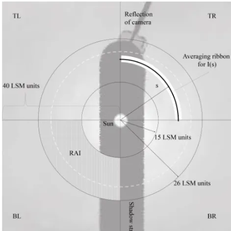
Figure 3.Layout of the local sky map (LSM). The LSM is divided into four quadrants, named according to their position as TR – top right, BR – bottom right, BL – bottom left, and TL – top left. The RAI is the radial analysis interval for which PST and IHS properties are evaluated. The approximate position of the halo maximum is sketched in light gray. Shadow strip and camera are excluded from analysis.
Step (4) identifies the solar position and masks nonsky de-tails. The position of the sun is marked based on the geo-graphical position of the TSI and the Universal Time (UTC) of the image. Extraneous details, such as the shadow strip, the area outside the horizon circle, the camera, and the cam-era mount, are masked. Figure 2c and d show the image pro-duced by all these adjustments up to step (4). Since often the position of the sun is detectable in the image, the marked sun position serves to refine the calibrations described above.
In step (5), the standardized local sky map is created. A sketch of the layout of the LSM is provided in Fig. 3. The LSM provides a standard sky section, centered at the sun, oriented with the horizon at the bottom, and presented in the same units for all possible TSI images (independent on the resolution of the original). Units of measurement in the LSM are closely related to angular degrees but do not match per-fectly due to a zenith angle dependence of the azimuth arc length. The LSM is generated by rotating and cropping the image from step (4) to approximately within 40◦of the sun, with the sun at its center.
The side length of the LSM in pixels scales with the pre-viously determined horizon radiusRHin pixels and the
cor-responding maximum zenith angleθHin◦as
wLSM(pixels)=
RH(pixels) θH(degrees)
×40◦. (10)
Equation (10) provides a unit transformation between pixel positions and LSM units. For a TSI image of size 480 pixels×640 pixels, the LSM will have a size of approx-imately 240 pixels×240 pixels. For the earlier, smaller TSI images, the LSM has a size of approximately 140 pixels×
140 pixels. The unit scaling includes the calibration choices RH andθH; hence, there is a slight variation in LSM side
lengths. We eliminate the influence of the LSM sizes by per-forming all algorithm operations in standardized LSM units, which roughly correspond to angles of 1◦. In other words, all LSMs are equivalent to each other in terms of their LSM units but not in terms of pixel positions. Atθ=45◦, the arc length of azimuth angle φ is equivalent to the arc length of θ of same size; however, if θ> 45◦, the azimuth arc is stretched, requiring an additional horizontal compression to ensure equivalence of horizontal and vertical angular units. The LSM is divided into quadrants, shown in Fig. 3, which are analyzed and classified separately by the algorithm de-scribed in the next section.
3.3 Computing photographic sky type and halo properties
3.3.1 Average radial intensity (ARI)
properties of I (s)to assign numeric PSTS and IHS, as de-tailed below.
The average radial intensityI (s)is computed as an aver-age over pixels at constant radial distancesfrom the sun. Due to the low resolution of the LSM, and due to some noise in the data, we averageI (s)over a circular ribbon with a width of 4 pixels, centered ats. ComputingI (s)over a thin ribbon addresses issues encountered when averaging over a circle in a coarse square grid, allowing continuity where otherwise pixelation may interrupt the line of the circle. Figure 4 shows the radial intensity of the red channel (R) in the bottom right quadrants of the LSMs featured in Fig. 2. Panel a includes I (s), a linear fit, as well as the running averageI6, plotted
versus radial distances. The running average is taken as the average ofI (s)over a width of 6 LSM units centered ats: I6(s)=
1 N
Xs+3 LSM units
s−3 LSM unitsI (s) . (11)
The clear-sky image exhibits a lower red intensity overall than the halo image. The halo presents as a brightness fluc-tuation at about 21 LSM units. The analysis ofI (s)is under-taken in an interval between 15 and 26 LSM units, called the radial analysis interval (RAI). The RAI is marked in Fig. 3. A linear fit yields a slope and intercept value used for the PSTS. We define the radial intensity deviation as
η (s)=I (s)−I6(s) . (12)
Panels b in Fig. 4 showη(s)for both situations. The details of the halo signal inη(s)contribute in particular to the com-putation of the IHS.
3.3.2 Photographic sky type (PST)
The training sets for the properties of I (s)were started for the set of 80 seed images mentioned in Sect. 1. Twenty im-ages for each sky type were divided further by sky quadrants, yielding between 60 and 80 property sets for each sky type to initiate the training sets. Some quadrants were eliminated by near-horizon sun positions. The training quadrants were used to apprise the utility ofI (s)in making sky type assignments, with focus on the radial analysis interval between 15 and 26 LSM units. The 10 image properties used to compute the nu-meric PSTS are listed in Table 3. Also listed are the compo-nents ofMtogether with their standard deviations, computed from a later and more complete version of the training sets. The 10 image properties include the slope and intercept of the line fit toI (s)for each color channel, where the slope charac-terizes a general brightness gradient, and the intercept gives access the overall brightness in the RAI. The line fit alone will not allow one to differentiate partially cloudy skies from other sky types. However, the presence of sharply outlined clouds leads to a larger variation in intensity values, even for the same radial distance from the sun. The areal standard de-viation (ASD) is an average of the standard dede-viation ofI (s) for each radial distances, averaged over all radii separated
by color channel. To set apart clear skies, the average color ratio (ACR) in the analysis area is computed as
ACR= B 2
GR. (13)
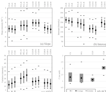
In Fig. 5, the PST property set is represented graphically, in-cluding means, standard deviations, and extreme values as observed for the completed training set. Clearly, no single property alone will suffice to assign a PST reliably. There is overlap in the extreme ranges. Relations between the color channels are influential as well. We are using the mechanism described in Sect. 2.1, Eqs. (1) through (6). The training sets for each class are collected in a master table, whereM and 6−1 for each PST are computed. As a new image is pro-cessed, and its PST property vectorXis computed for each sky quadrant. Subsequently, a numeric score is computed for each sky type using Eq. (6). The coefficientC0 in Eq. (6)
for the PSTS computation is chosen as 103, which places a rough separator of order 1 between images that match closely a particular sky type and those which do not. The raw values ofFimagein Eq. (6) vary greatly even between similar
look-ing images; hence the PSTS is computed as a relative con-tribution between 0 % and 100 % for each sky type and each quadrant. For the PST-CS score this would mean
PST_CS= FCS
FCS+FPCL+FCLD+FCLR
Figure 4.Average radial intensity of the red channel is shown versus radial distances, measured in LSM units, for the two images of Fig. 2, halo at left.(a)includes the average intensityI (s), a linear fit, and the running averageI6(s)as averaged over a width of 6 LSM units.
(b)shows the radial intensity deviationη (s). The halo signal is visible as a minimum at 17 LSM units, followed by a maximum at 21 LSM units in the left column.
Table 3.Discriminant properties used to classify the photographic sky type. Averages and standard deviations for the training set of each class are listed. All units are based on color intensity values and LSM units. The number of records for each sky type is indicated in parentheses.
PST property PST-CS (155) PST-PCL (99) PST-CLD (93) PST-CLR (96)
Slopea B−3.0±1.5 B−1.6±2.2 B−0.7±1.7 B−2.3±1.6 G−3.2±1.7 G−1.6±2.2 G−0.7±1.7 G−2.8±1.6 R−3.6±1.9 R−1.9±2.6 R−0.8±1.8 R−2.8±1.7
Interceptb B 276±34 B 248±46 B 193±40 B 248±43 G 271±33 G 240±53 G 195±44 G 233±47 R 255±48 R 228±65 R 179±47 R 184±47
ASD1 B 13.1±5.3 B 20.5±7.0 B 14.2±5.0 B 15.4±5.2 G 15.0±6.0 G 22.9±7.7 G 15.0±5.1 G 16.3±5.3 R 16.6±6.6 R 25.5±8.1 R 15.8±5.6 R 14.8±5.7
ACR2 1.33±0.36 1.24±0.32 1.08±0.12 2.07±0.11
1Areal standard deviation.2Average color ratio.
PST-CS and PST-PCL, and the images corroborate this. The 14:36:00 image shows a thicker cloud cover, and the algo-rithm correctly responds by increasing the PST-CLD score. At 21:00:00, the algorithm indicates an increased PST-CLR score, consistent with the visual inspection of the TSI im-age at the time. Given the simplicity and physical relevance of this photographic sky type assessment, we believe that a radial scattering analysis around the sun has the potential
Figure 5.Photographic sky type properties. Slope and intercept(a, b)for the radial fit; areal standard deviation (ASD) of brightness(c); average color ratio (ACR)(d). Sky types were assigned visually.
2016; Long et al., 2006). That will be a direction to discuss and explore in the future.
3.3.3 Ice halo score (IHS)
The 22◦halo is a signal in the image that can be obscured by many other image features, including low clouds, partial clearings, inhomogeneous cirrostratus, regions of overexpo-sure, and near-horizon distortions. The appearances of 22◦ halos span a wide variety of sky conditions, ranging from almost clear skies to overcast altostratus skies, with the ma-jority of halo phenomena appearing in cirrostratus skies. The challenge to extract the halo from such a wide variety of sky conditions is formidable. While the statistical approach de-scribed in Sect. 2.1 will again form the core of the approach, the challenge shifts to defining a set of suitable discriminat-ing properties of the image. In addition to the properties used in sky type assignment, the halo scoring must seek features in η(s), Eq. (12), that are unique in halo images, such as a minimum followed by a maximum at halo distance from the sun. The absolute values of η(s)are dependent on vari-ous image conditions. Due to the variety of sky conditions, and variations in calibration and image quality, the values of maximum and minimum alone are not sufficient to re-liably conclude the presence of a halo. We have found in-stances in which η(s) does exhibit the halo maximum but
does not dip to negative values first. However, the upslope– crest–downslope sequence is consistently present in all cases of 22◦ halo. The halo search is undertaken for a sequence of upslope–crest–downslope in terms of radial positions and range of slopes. All three characteristics present clearly in the derivative of theη(s), the radial intensity deviation derivative η0(s). This derivative of the discrete seriesη(s)is approxi-mated numerically by a secant method as
η0i≈ηi+1−ηi−1
si+1−si−1
. (15)
In Fig. 7, bothη(s)andη0(s)are shown for the bottom-right quadrant of the green channel of the halo image in Fig. 2. The sequence of radial halo markers is illustrated in Fig. 7. The algorithm computesη0(s)and seeks the positive maximum and the subsequent negative minimum, plus the ra-dial position of the sign change between them. This produces a sequence of radial locationssup,smax, andsdownwhich
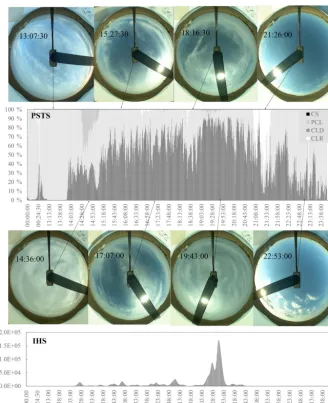
Figure 6.The 1 d example for PSTS and IHS (SGP 10 March 2018). Sample TSI images are included. The middle panel shows PSTS versus time of day (N/A excluded). Bottom panel shows the IHS versus time;w=3.5 min. All times in UTC.
Table 4.Discriminant properties used for the ice halo score. Averages and standard deviations for a training set of 188 quadrant records are listed. All units are based on color intensity values and LSM units.
IHS property B G R
Slopea −3.3±1.5 −3.3±1.6 −3.8±1.8 Interceptb 279±35 278±37 268±45 ASD 12.6±4.7 14.8±6.0 16.2±6.4 Maximum upslopeη0up 2.1±1.3 2.1±1.4 2.5±1.6 Maximum downslopeη0down −1.6±1.0 −1.6±1.0 −1.8±1.1 Upslope locationsup 17.5±1.9 17.8±2.3 17.5±2.1
Maximum locationsmax 18.9±1.9 19.1±2.3 18.8±2.1
Downslope locationsdown 20.0±2.1 20.2±2.4 19.9±2.2
Number of maximanmax 2.4 2.6 2.5
BGR consistency σBGR sup=0.8 σBGR(smax)=0.8 σBGR(sdown)=0.9
Figure 7.Radial markers used in halo scoring. The data belong to the green channel of the TSI image from SGP, 17 April 2018; see Fig. 2.
(a)shows the radial intensity deviationη (s);(b)shows its derivativeη0(s). Units are color value units (0 to 255) for the intensity and LSM units for the radial distance. The sequence of radial locations used in halo scoring is indicated, as well as the interpretation of the up- and downslope markers.
should be consistent across all three color channels. The res-olution of the TSI images only allows one to resolve 0.4 to 1.2◦with certainty; in addition, variations in calibration and SZA do influence deviations from the expected 22◦position. The separation of colors observed in a 22◦halo display is not resolved with statistical significance; therefore this was not used as a criterion for halo detection. The standard deviation of all three radial positions across the three color channels was added to the halo scoring set of properties. We arrive at a set of 31 properties for the computation of the IHS, listed in Table 4, together with their means and standard deviations. The mean value vectorM and the inverse covariance matrix 6−1are computed in the master table and then imported by the halo searching algorithm for use in Eq. (6). The coeffi-cient C0 in Eq. (6) is arbitrary. In the IHS computation, a
value of 106 was chosen forC0, which places a rough
sep-arator of order 1 between image quadrants that do have a halo and those which do not. While the scoring of individual images works very well for true halo images, it does trig-ger the occasional halo score for images that do not exhibit a halo. This may occur due to inhomogeneities in a broken cloud cover or other isolated circumstances. These false halo scores often occur on isolated images. We utilize the factor of residence time of a halo to address this. In a 30 s binned se-ries of TSI images, the halo will appear usually in a sequence of subsequent images, often in the order of minutes or even hours. We added a Gaussian broadening to the time series of
halo scoresFi,taken at timesti with a broadeningw:
IHS(t )= ti=t+3w
X
ti=t−3w
F (ti)exp "
−(ti−t ) 2
2w2 #
. (16)
This de-emphasizes isolated instances and enforces se-quences of halo scores, even if they individually exhibit weak signals or gaps. This procedure reduced the false halo iden-tifications significantly. Just as for the PSTS, the training set for the IHS in the master table is being complemented as more images are analyzed. The raw halo scoreF is com-puted for each of the four quadrants of an individual image; their average is used to assign the raw score for the whole im-age. The broadening in Eq. (16) was chosen asw=7 images throughout, corresponding to 3.5 min. In Fig. 6, the clear 22◦ halo between 19:00 and 20:00 UTC produces a strong IHS. There are a few weaker halo signals, and upon inspection of the images we find that these correspond to partial halos (like at 17:07:00), or halos in a more variable sky.
4 Results for January through April 2018
classifiable in terms of their PST. Exclusions occur due to large SZA, overexposure, or low PSTS.
The algorithm and the current training set (starting with the 80 sets discussed above) are used to assign an image IHS and a set of four image PSTS, averaging over the quadrant IHS and PSTS values. Both of these score sets are contin-uous numerical values, resulting in a time-resolved scoring for all PSTS and IHS values as shown in Fig. 6, across the month of March. In order to manage comparison to a visual classification of these images, and to learn how both score sets behave in terms of numerical values, the following two procedural steps are added in the postprocessing: (1) for the PST, the sky type with the maximum contribution is taken as the image sky type; (2) an IHS discriminator is used to assign a halo/no halo designator to an image. This IHS discrimina-tor is arbitrary, not part of the image analysis algorithm, and dependent on factors such as w and C0, the quality of the
calibration, and the quality and relevance of the training set. The algorithm assigns a continuous IHS to every image as a number varying between 10−10and 106, with fluid continu-ous change in consecutive images. The decision on the value of the discriminator is based on the behavior of the timeline. Halo images generate a significant peak above a population of low-level peaks. The discriminator is placed to exclude about 75 % of the low peaks when analyzing for a count of halo incidences. Our testing, minimizing false negatives and maximizing correct positives, places it at around 4000 for the month of March.
Visual image classification for so many images poses a considerable challenge, which we approached in the form of an iteration. For each of the 31 d of March, an observer as-signed sky classifications to segments of the day by inspect-ing the day series as an animation. This can easily be done by using an image viewer and continuously scrolling through the series. Then, the day would be subjected to the algorithm. The sections of the record in which visual and algorithm dif-fered were inspected again, at which point either the visual assessment was adjusted or samples of the misclassified im-ages were added to the training set. Adjustment to visual classifications often occurred at the fringes of a transition. For example, when a sky transitions from cirrostratus to alto-stratus to alto-stratus, the transitions are not sharp. The observer sets an image as the point in which the sky moved from PST-CS to PST-CLD, but the criteria in the algorithm would still indicate PST-CS. This can affect up to a hundred images at transition times, which then were reclassified. On the other hand, if a clearly visible halo was missed by the algorithm in the form of a low numerical IHS, a couple of new lines were added to the training set, selected from the few hundred quadrant cases in which this particular halo had scored low. The IHS discriminator is not part of the algorithm itself, but follows in the postprocessing from the general behavior of the IHS across the month. It is a tool to allow a comparison but not an ultimate answer to halo strength. Halo strength could be assessed by the IHS. After each change to the
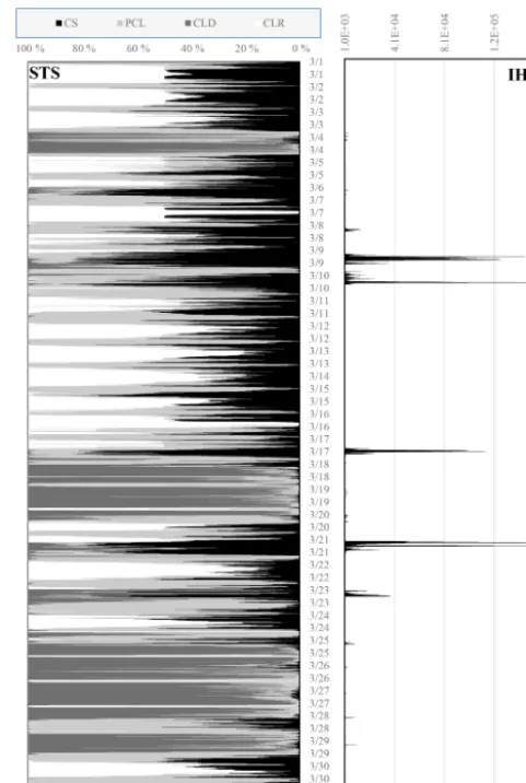
train-Figure 8.PSTS and IHS versus time for TSI images from SGP March 2018. Left panel shows the PSTS. Right panel: IHS broad-eningw=3.5 min.
ing set, the algorithm would be repeated, and recalibrations to the visual record, as well as to the training set, were made. The process was repeated several times until no more gains in accuracy were observed. The training sets at the end of this process contained between 93 and 188 property records, of which up to 50 % were taken from March 2018. Com-pared to the number 31 398 of classifiable images in March (after exclusion of high-SZA, overexposure, and other), and considering that each of these images contributes up to four individual property sets, the number of training sets is indeed diminutive. These adjustments were done by SB.
Table 5.Algorithm versus visual classifications for SGP March 2018.(a)shows the percentage of visual assignments corresponding to algorithm assignments; (b)shows the percentage of algorithm assignments and how they distribute among the visual assignments. For example, 88 % of all visual CS skies are classified as PST-CS by the algorithm, but only 86 % of all algorithm PST-CS skies also identify as visual CS. Agreement combinations are shown in bold. A halo was assigned to an image if IHS > 4000.
(a) Percentage of visually assigned sky type which corresponds to algorithm-assigned PST
CS PCL CLD CLR
N % N % N % N %
PST-CS 6675 88 683 11 38 1 397 4 PST-PCL 182 2 5513 86 176 3 191 2 PST-CLD 61 1 47 1 6129 97 0 0 PST-CLR 641 8 136 2 0 0 10 529 95
N/A 12 597 (40 % of all images)
Percentage of visually assigned halos which corresponds to
the algorithm assignment
22◦halo No 22◦halo
N % N %
22◦halo 1996 85 272 1 No 22◦halo 349 15 41 409 99
(b) Percentage of algorithm-assigned PST which corresponds to a visually assigned sky type
CS PCL CLD CLR
N % N % N % N %
PST-CS 6675 86 683 9 38 0 397 5 PST-PCL 182 3 5513 91 176 3 191 4 PST-CLD 61 1 47 1 6129 98 0 0 PST-CLR 641 6 136 1 0 0 10 529 93
N/A 12 597 (40 % of all images) Percentage of algorithm-assigned assigned halos which corresponds
to a visual assignment
22◦halo No 22◦halo
N % N %
22◦halo 1996 88 272 12 No 22◦halo 349 1 41 409 99
In Table 5, visual and algorithm results of the sky type as-signments are cross-listed for SGP March 2018. It is worth reminding the reader that PSTs are assigned only for the ra-dial analysis interval indicated in Fig. 3. Table 5a lists the percentage of visually assigned sky types that correspond to the algorithm-assigned PST; Table 5b lists the percentage of algorithm-assigned PSTs that also have been identified as a visual sky type. For example, the algorithm correctly identi-fies 88 % of all visual CS skies as PST-CS (part A); 86 % of the images classified as PST-CS by the algorithm also have been visually classified as CS (part B). PST-CLD is re-liably identified by the algorithm. A small percentage (3 %)
pos-sible that the visual assignments carry a considerable uncer-tainty. Some of the visual PST-CS skies, for example, present to the eye as PST-CLR but reveal the movement of a thin cirrostratus layer if viewed in the context of time develop-ment (animation). Similarly, cirrostratus may present as an inhomogeneous layer in transition skies, triggering a PST-PCL assessment in the algorithm. Low solar positions are prone to larger image distortion, which may lead to misin-terpretation. It is worth noting that every image quadrant re-ceives a PSTS for all classes of PST. In cases of mismatch, we often find that the two sky types at conflict both con-tribute significantly to the PSTS of the image quadrant. If SZA > 68◦, no PST assignments were made. Most of the 397 PST-CLR images that presented as PST-CS to the algorithm were taken at very low sun, with a significant overexposure disk in near-solar position. Table 5 also lists a comparison of visual halo identifications with the algorithm scores. Ac-cording to this assessment, the algorithm correctly calls 85 % of visual halo images while not diagnosing 15 % of them. On the other hand, 12 % of all halo signals do not correspond to a halo in the image. One can improve the correct identification rate by lowering the cutoff score, at the cost of an increase in the signal from false identifications. Balancing the false positive and false negatives yields a reliability of about 12 % to 14 %. Some of the false negatives arise from altocumu-lus skies, in which the outlines of cloudlets may trigger halo signals by their distribution and size. These are very difficult to discriminate from visual halo images. Some images were flagged with an IHS by the algorithm, and the presence of a weak halo revealed itself only after secondary and tertiary inspection of the image. Caution is advised in relying heavily on visual classifications of TSI images alone. The visual sky type and halo assignments themselves have an uncertainty due to subjectivity. While it is easy to distinguish a partially cloudy sky from a clear sky, this may become difficult for the difference between thick cirrostratus and stratus. Their visual appearances may be quite similar. Sometimes, an as-signment can be made in the context of temporal changes. Some clear-appearing skies reveal a thin cirrostratus pres-ence if viewed in a time series instead of in an individual image. It is therefore a future necessity to combine the vi-sual assignments of sky types with lidar data for altitude, optical thickness, and depolarization measurements to make an accurate assessment of the efficacy of the PST identifica-tion, following closely the processes described by Sassen et al. (2003) and Forster et al. (2017).
We applied the algorithm to the TSI record for the first 4 months of 2018 for the SGP ARM site. It is worth not-ing that this paper is not intended to present a complete ex-ploration of the ARM record concerning 22◦halos. We are, however, including a demonstration of capacity of the algo-rithm presented here. Table 6 summarizes our findings. It lists the percentages for the PST by month. A portion of the images has not been assigned with a PSTS. The conditions under which this occurs have been described earlier and
in-clude near-horizon sun positions, images with overexposure in the RAI, and images for which the raw PSTS for each sky type was numerically too low to be considered a reliable as-sessment. Therefore, PST percentages refer only to all identi-fied images. January and March exhibited a large fraction of clear skies. February was dominated by cloudy skies, while April registered a high percentage of PST-CS. Only a partial month of images was available for April. Cloud types depend strongly on the synoptic situation. That means that no further conclusions should be made from these data without expand-ing the data set. The 22◦halo statistics in Table 6 lists data on the 22◦halo, including duration, number of incidents, and data on partial halos. The partial halo data are based on the individual quadrant IHS for an image, while the image score is used for duration and incidence information. The number of separate halo incidences counts sequences of images for which the IHS did not fall below the cutoff value of 4000. While it is worth noting that the number of incidences lies in the order of magnitude of the number of days in a month, it is certain that the halo instances are not evenly distributed. Figure 8 does demonstrate this behavior. However, even on a day of persistent cirrostratus with 22◦ halo, interruptions of its visibility can occur. Sometimes low stratocumulus may obscure the view of the halo, and sometimes the cirrus layer is not homogeneous. This may lead to a large number of sep-arate halo incidences in a short time, while none are counted at other times. The mean duration of a halo incident lies be-tween 16 and 34 min, depending on month. We listed the maximum duration found in each month as well. The longest halo display in the time period occurred in April 2018, with nearly 3.5 h. Mean values are easily skewed by a few long-lasting displays. Figure 9 shows the distribution of 22◦halo durations for the 4 months. The most common duration of a 22◦ halo lies between 5 and 10 min, followed by 10 to 15 min. Due to the time broadening applied via Eq. (16), the display time cannot be resolved below 3 min. We consider the fraction of images in which a halo was registering. That marker varied between 3.9 % for January and 9.4 % for April. In accord with findings in Sassen et al. (2003), we find a low amount of halo display activity in January. However, this may be influenced by the large SZA in January. The closer the sun to the horizon, the more TSI images have been excluded from the analysis, and the stronger the influence of distortion.
Table 6.PST and 22◦halo formations during the months of January through April 2018 (SGP). Percentages are with respect to all classifiable images. Times are in UTC.
Jan 2018 Feb 2018 Mar 2018 Apr 2018∗
Total number of images 36 632 36 011 44 057 27 741 Number with valid PST 21 238 23 604 31 398 20 436
Begin date of record 1 Jan 2018 13:47:00 1 Feb 2018 13:36:00 1 Mar 2018 0:00:00 1 Apr 2018 0:00:00 End date of record 31 Jan 2018 23:50:00 28 Feb 2018 23:59:30 31 Mar 2018 23:59:30 19 Apr 2018 1:02:00
PST
PST-CS 20 % 18 % 25 % 34 %
PST-PCL 24 % 24 % 19 % 19 %
PST-CLD 11 % 33 % 20 % 25 %
PST-CLR 45 % 25 % 36 % 22 %
22
◦halos
Number of separate 26 45 34 46
halo incidents
Mean duration 16 min 22 min 34 min 21 min Maximum duration 62 min 136 min 171 min 208 min Total halo time 411 min 998 min 1160 min 963 min % halo instances with
4/4 22◦halo 29 % 42 % 77 % 42 % 1/3 22◦halo 38 % 31 % 13 % 40 % 1/2 22◦halo 32 % 25 % 10 % 18 %
1/4 22◦halo 1 % 1 % 0 % 0 %
Relations
% halo instances of all sky type instances
PST-CS 9 % 16 % 18 % 22 %
PST-PCL 6 % 7 % 6 % 9 %
PST-CLD 4 % 5 % 10 % 12 %
PST-CLR 0 % 0 % 0 % 0 %
All PSTSs 3.9 % 8.5 % 7.4 % 9.4 % % sky type of all
halo instances
PST-CS 49 % 60 % 87 % 78 %
PST-PCL 42 % 33 % 9 % 14 %
PST-CLD 2 % 5 % 3 % 5 %
PST-CLR 0 % 0 % 0 % 0 %
N/A 7 % 2 % 1 % 3 %
∗Incomplete month.
We started the project with the goal to find information on cirrostratus composition, in particular with respect to assess-ments of variation of smooth versus rough crystals. Forster et al. (2017) discuss that the necessary fraction of smooth crys-tals for a halo appearance lies between 10 % and 40 %. The bottom part of Table 6 investigates the relation between sky type and 22◦halo incidences. The first set of data in the “Re-lations” section of Table 6 gives the fraction of each sky type, as it produced a 22◦halo incident. For example, in January we found that 9 % of PST-CS were accompanied by a 22◦ halo. In the data for April, this fraction increased to 22 % of CS. We also have registered halos for a portion of PST-PCL and for PST-CLD. No halos have been registered in any of the PST-CLRs. The April data are consistent with the ob-servations of Forster et al. (2017), who report a 22◦halo for 25 % of all cirrus clouds for a 2.5-year photographic record taken in Munich, Germany. Differences exist, however, in that the Forster observations verified ice cloud with lidar and IR measurements, while this current record compares to a photographically assigned sky type. We must consider rea-sons for the PST-PCL and PST-CLD halo incidences. Upon random sampling of these combinations we find the follow-ing: the PST-PCL indicator has been assigned to images that have a highly varied cirroform sky, including halo appear-ances. In a few instances, low clouds triggered the PST-PCL indicator; however, a cirroform layer at higher altitude still contributed a halo score above the threshold. Many of the halo scores in PST-CLD skies belong to images with an over-cast appearance; however, they most likely belong to a thick-ening and lowering cirro- or altostratus as is often found in warm front approaches. These are not false scores but condi-tioned by the limitations of the PST classification. The sec-ond set of numbers in Table 6 shows the fraction of all ha-los associated with the various PST. In January, 49 % of all halo incidences occurred in PST-CS skies, while in March this number was 87 %. As for the overall frequency of halo displays, we can refer to Table 6, in which the observed halo frequency for all PST combined is listed. It varies from 3.9 % in January 2018 to 9.4 % in April 2018. The closest compar-ison is the number given by Sassen et al. (2003), who report a full 22◦halo at 6 % of the 10-year record of hourly images, while any halo feature was observed at 37.3 % of the time. For such a comparison, Forster et al. (2017) is cautioning that a statistic like this may strongly depend on the binning interval.
With this image analysis algorithm used on TSI images to identify the PST and the appearance of 22◦ halos, the next useful and logical step will be to relate these data to other in-strument records: lidar for altitude, particle density, and par-ticle phase (solid or liquid), as well as photometric measure-ments to glean information on radiative flux. ARM sites have accumulated such instrumental data. The algorithm proposed here will make such data investigation possible.
Finally, it is worth discussing the general approach of the TSI algorithm in comparison to the halo detection algorithm
developed by Forster et al. (2017). Both algorithms utilize features found in the radial intensityI (s), such as the se-quence of minimum–maximum at the expected radial posi-tions in order to find halos in an image. The random forest classifier approach described in Forster et al. (2017) is a ma-chine learning approach that arrives at a binary conclusion for an image in the form of halo/no halo. Their algorithm was trained on a visually classified set of images in order to construct a suitable decision tree. In addition to 22◦ halos, the Forster algorithm also identifies parhelia and other halo display features in images taken by a high-resolution, sun-tracking halo camera. The algorithm presented here for TSI data must work with a much less specialized set of images, notably of lower resolution. It does not characterize halos in a binary decision but rather assigns a continuous ice halo score to an image, in addition to photographic sky type scores for four different types of sky conditions. Similar to the Forster algorithm, the TSI algorithm also was trained on a visually classified set of images. For the algorithm presented here, further training sets are easily added. Both algorithms have overlap. The TSI algorithm makes extensive use of the radial brightness gradient (slope) for the sky type assignments. The relation of this gradient to the physical presence of scatterers along the optical path makes this an attractive approach.
5 Summary
displays, with a most common duration of about 5 to 10 min but lasting up to 3 h. It allowed us to identify the fraction of PST-CS skies that do produce halo displays, as well as find such data for other PST. In the future, the algorithm will be applied to deliver 22◦halo data for the long-term TSI records accumulated in various geographical locations of ARM sites, as well as allow further investigation into correlations with other instrumental records from those sites. In particular, li-dar data for altitude and optical thickness measurements, as well as depolarization analysis, will be a useful combination with this photographic halo display record. It is reasonable to expect that the reference set for sky type determination will improve with the support of lidar data. The method described here may be suitable to expand to other types of sky analysis on TSI images.
Code availability. Code and accessory files are made available at GitHub under https://doi.org/10.5281/zenodo.2226125 (Boyd et al., 2018).
Author contributions. SB is the main author of this paper and the code. The four coauthors worked on the algorithm as undergraduate researchers. SS decided on the use of C++and OpenCV3.2 for image manipulation and initiated the program code. SR worked out the details of the radial intensity computation and properties. MK and MG contributed algorithm parts to eliminate optical distortions and low-cloud obstruction, as well as input management. SR, MK, and MG all contributed to data collection and analysis.
Competing interests. The authors declare that they have no conflict of interest.
Acknowledgements. Data were obtained from the Atmospheric Ra-diation Measurement (ARM) Program sponsored by the U.S. De-partment of Energy, Office of Science, Office of Biological and En-vironmental Research, Climate and EnEn-vironmental Sciences Divi-sion. The work was supported by The Undergraduate Research Op-portunities Program (UROP) at the University of Minnesota, as well as a grant to the University of Minnesota Morris from the Howard Hughes Medical Institute through the Precollege and Undergraduate Science Education Program. Sylke Boyd wishes to thank the Uni-versity of Minnesota Morris for the generous one-semester release from teaching obligations, allowing for the completion of this work.
Review statement. This paper was edited by Andrew Sayer and re-viewed by two anonymous referees.
References
Alpaydin, E.: Introduction to machine learning, third edition, Cam-bridge, Mass, MIT Press, CamCam-bridge, Mass, 2014.
Atmospheric Radiation Measurement (ARM): Climate Research Facility. updated hourly. Total Sky Imager (TSISKYIMAGE). 2013-10-01 to 2018-05-28, Eastern North Atlantic (ENA) Gra-ciosa Island, Azores, Portugal (C1). 2006-04-25 to 2018-04-11, North Slope Alaska (NSA) Central Facility, Barrow AK (C1). 2013-08-30 to 2018-05-24, ARM Mobile Facility (OLI) Olikiok Point, Alaska; AMF3 (M1). 2000-07-02 to 2018-04-19, Southern Great Plains (SGP) Central Facility, Lamont, OK (C1), compiled by: Morris, V., Atmospheric Radiation Measurement (ARM) Cli-mate Research Facility Data Archive: Oak Ridge, Tennessee, USA, https://doi.org/10.5439/1025309, 2000.
Bailey, M. P. and Hallett, J.: A Comprehensive Habit Diagram for Atmospheric Ice Crystals: Confirmation from the Laboratory, AIRS II, and Other Field Studies, J. Atmos. Sci., 66, 2888–2899, 2009.
Baran, A.: A review of the light scattering properties of cirrus, J. Quant. Spectrosc. Ra., 10, 1239–1260, 2009.
Boyd, S., Sorenson, S., Richard, S., King, M., and Greenslit, M.: Haloloop-Search TSI record for ice halos, Zenodo, doi.org/10.5281/zenodo.2226125, 2018.
Calbó, J. and Sabburg, J.: Feature Extraction from Whole-Sky Ground-Based Images for Cloud-Type Recognition, J. Atmos. Ocean. Tech., 25, 3–14, 2008.
Campbell, J. R., Lolli, S., Lewis, J. R., Gu, Y., and Welton, E. J.: Daytime Cirrus Cloud Top-of-the-Atmosphere Radiative Forcing Properties at a Midlatitude Site and Their Global Consequences, J. Appl. Meteorol. Clim., 55, 1667–1679, 2016.
Cziczo, D. J. and Froyd, K. D.: Sampling the composition of cirrus ice residuals, Atmos. Res., 142, 15–31, 2014.
Fasullo, J. T. and Balmaseda, M. A.: Earth’s Energy Imbalance, J. Climate, 27, 3129–3144, 2014.
Fasullo, J. T. and Kiehl, J.: Earth’s Global Energy Budget, B. Am. Meteorol. Soc., 90, 311–324, 2009.
Fasullo, J. T., von Schuckmann, K., and Cheng, L.: Insights into Earth’s Energy Imbalance from Multiple Sources, J. Climate, 29, 7495–7505, 2016.
Flury, B.: Multivariate statistics: a practical approach, London, New York: Chapman and Hall, London, New York, 1988.
Forster, L., Seefeldner, M., Wiegner, M., and Mayer, B.: Ice crys-tal characterization in cirrus clouds: a sun-tracking camera sys-tem and automated detection algorithm for halo displays, At-mos. Meas. Tech., 10, 2499–2516, https://doi.org/10.5194/amt-10-2499-2017, 2017.
Fu, Q., Lohmann, U., Mace, G. G., Sassen, K., and Com-stock, J. M.: High-Cloud Horizontal Inhomogeneity and So-lar Albedo Bias, J. Climate, 15, https://doi.org/10.1175/1520-0442(2002)015<2321:HCHIAS>2.0.CO;2, 2002.
Ghonima, M. S., Urquhart, B., Chow, C. W., Shields, J. E., Cazorla, A., and Kleissl, J.: A method for cloud detection and opacity classification based on ground based sky imagery, Atmos. Meas. Tech., 5, 2881–2892, https://doi.org/10.5194/amt-5-2881-2012, 2012.
Gnanadesikan, R.: Methods for statistical data analysis of multivari-ate observations, New York, Wiley, New York, 1977.
Greenler, R.: Rainbows, Halos, and Glories, Cambridge University Press, Cambridge, 1980.
sky conditions using a fractal cloud model, Sol. Energy, 150, https://doi.org/10.1016/j.solener.2017.04.048, 2017.
Hammer, E., Bukowiecki, N., Luo, B. P., Lohmann, U., Mar-colli, C., Weingartner, E., Baltensperger, U., and Hoyle, C. R.: Sensitivity estimations for cloud droplet formation in the vicinity of the high-alpine research station Jungfrau-joch (3580 m a.s.l.), Atmos. Chem. Phys., 15, 10309–10323, https://doi.org/10.5194/acp-15-10309-2015, 2015.
Harris, R. J.: A primer of multivariate statistics, New York, Aca-demic Press, New York, 1975.
Heymsfield, A. J., Schmitt, C., and Bansemer, A.: Ice Cloud Particle Size Distributions and Pressure-Dependent Terminal Velocities from In Situ Observations at Temperatures from 0◦to−86◦C, J. Atmos. Sci., 70, 4123–4154, 2013.
Hong, Y., Liu, G., and Li, J.-L. F.: Assessing the Radiative Effects of Global Ice Clouds Based on CloudSat and CALIPSO Mea-surements, J. Climate, 29, 7651–7674, 2016.
Ilie, A. and Welch, G.: Ensuring color consistency across multiple cameras, Tenth IEEE International Conference on Computer Vi-sion (ICCV’05) Volume 1, 1262, 1268–1275, 2005.
IPCC: Climate Change 2013: The Physical Science Basis, Contri-bution of Working Group I to the Fifth Assessment Report of the Intergovernmental Panel on Climate Change, Cambridge, UK and New York, USA, 1535 pp., 2013.
IPCC: Climate Change 2014: Synthesis Report. Contribution of Working Groups I, II and III to the Fifth Assessment Report of the Intergovernmental Panel on Climate Change Geneva, Switzerland, 151 pp., 2014.
Kandel, R. and Viollier, M.: Observation of the Earth’s radiation budget from space, Observation du bilan radiatif de la Terre depuis l’espace, 342, 286–300, 2010.
Kennedy, A., Dong, X., and Xi, B.: Cloud fraction at the ARM SGP site: reducing uncertainty with self-organizing maps, Theor. Appl. Climatol., 124, 43–54, 2016.
Knobelspiesse, K., van Diedenhoven, B., Marshak, A., Dunagan, S., Holben, B., and Slutsker, I.: Cloud thermodynamic phase de-tection with polarimetrically sensitive passive sky radiometers, Atmos. Meas. Tech., 8, 1537–1554, https://doi.org/10.5194/amt-8-1537-2015, 2015.
Kollias, P., Tselioudis, G., and Albrecht, B. A.: Cloud climatol-ogy at the Southern Great Plains and the layer structure, drizzle, and atmospheric modes of continental stratus, J. Geophys. Res.-Atmos., 112, https://doi.org/10.1029/2006JD007307, 2007.
Long, C. N., Sabburg, J. M., Calbó, J., and Pagès, D.: Retrieving Cloud Characteristics from Ground-Based Daytime Color All-Sky Images, J. Atmos. Ocean. Tech., 23, 633–652, 2006. Sassen, K.: Corona-producing cirrus cloud properties derived from
polarization lidar and photographic analyses, Appl. Opt., 30, 3421–3428, 1991.
Sassen, K., Zhu, J., and Benson, S.: Midlatitude cirrus cloud clima-tology from the Facility for Atmospheric Remote Sensing. IV. Optical displays, Appl. Opt., 42, 332–341, 2003.
Schwartz, S. E., Charlson, R. J., Kahn, R., and Rodhe, H.: Earth’s Climate Sensitivity: Apparent Inconsistencies in Recent Assess-ments, Earth’s Future, 2, 601–605, 2014.
Tape, W. and Moilanen, J.: Atmospheric Halos and the Search for Angle X, Am. Geophys. Un., 2006.
Tian, L., Heymsfield, G. M., Li, L., Heymsfield, A. J., Bansemer, A., Twohy, C. H., and Srivastava, R. C.: A Study of Cirrus Ice Par-ticle Size Distribution Using TC4 Observations, J. Atmos. Sci., 67, 195–216, 2010.
Trenberth, K. E., Zhang, Y., and Fasullo, J. T.: Relationships among top-of-atmosphere radiation and atmospheric state variables in observations and CESM, J. Geophys. Res.-Atmos., 120, 10074– 10090, 2015.
Um, J. and McFarquhar, G.: Formation of atmospheric halos and applicability of geometric optics for calculating single-scattering properties of hexagonal ice crystals: Impacts of aspect ratio and ice crystal size, J. Quant. Spectrosc. Ra., 165, 134–152, 2015. van Diedenhoven, B.: The prevalence of the 22 deg halo in cirrus
clouds, J. Quant. Spectrosc. Ra., 146, 475–479, 2014.
van Diedenhoven, B.: The effect of roughness model on scattering properties of ice crystals, J. Quant. Spectrosc. Ra., 178, 134–141, 2016.
Waliser, D. E., Li, J.-L. F., Woods, C. P., Austin, R. T., Bacmeis-ter, J., Chern, J., Del Genio, A., Jiang, J. H., Kuang, Z., Meng, H., Minnis, P., Platnick, S., Rossow, W. B., Stephens, G. L., Sun-Mack, S., Tao, W.-K., Tompkins, A. M., Vane, D. G., Walker, C., and Wu, D.: Cloud ice: A climate model challenge with signs and expectations of progress, J. Geophys. Res.-Atmos., 114, https://doi.org/10.1029/2008JD010015, 2009.