https://doi.org/10.5194/os-14-1373-2018 © Author(s) 2018. This work is distributed under the Creative Commons Attribution 4.0 License.
Modelling of ships as a source of underwater noise
Jukka-Pekka Jalkanen1, Lasse Johansson1, Mattias Liefvendahl2,3, Rickard Bensow2, Peter Sigray3, Martin Östberg3, Ilkka Karasalo3, Mathias Andersson3, Heikki Peltonen4, and Jukka Pajala4
1Atmospheric Composition Research, Finnish Meteorological Institute, 00560 Helsinki, Finland 2Mechanics and Maritime Sciences, Chalmers University of Technology, 41296 Gothenburg, Sweden
3Underwater Technology, Defence and Security, Systems and Technology, Swedish Defense Research Agency, 16490 Stockholm, Sweden
4Marine Research Centre, Finnish Environment Institute, 00790 Helsinki, Finland Correspondence:Jukka-Pekka Jalkanen ([email protected])
Received: 12 April 2018 – Discussion started: 19 April 2018
Revised: 28 September 2018 – Accepted: 3 October 2018 – Published: 7 November 2018
Abstract.In this paper, a methodology is presented for mod-elling underwater noise emissions from ships based on real-istic vessel activity in the Baltic Sea region. This paper com-bines the Wittekind noise source model with the Ship Traf-fic Emission Assessment Model (STEAM) in order to pro-duce regular updates for underwater noise from ships. This approach allows the construction of noise source maps, but requires parameters which are not commonly available from commercial ship technical databases. For this reason, alterna-tive methods were necessary to fill in the required informa-tion. Most of the parameters needed contain information that is available during the STEAM model runs, but features de-scribing propeller cavitation are not easily recovered for the world fleet. Baltic Sea ship activity data were used to gen-erate noise source maps for commercial shipping. Container ships were recognized as the most significant source of un-derwater noise, and the significant potential for an increase in their contribution to future noise emissions was identified.
1 Introduction
It is recognized that anthropogenic noise might have adverse effects on the marine environment. Scientific results unequiv-ocally suggest that animals react to sound – sometimes with devastating results (Rolland et al., 2012; Yang et al., 2008), but more commonly sound gives rise to strong avoidance reactions (Moore et al., 2012). Not all marine life is sensi-tive to the same kind of noise; low-frequency shipping noise (<1000 Hz) may be relevant for several fish species, whereas
this range may be less relevant for marine mammals that can hear sounds up to 200 kHz (Nedwell et al., 2004). The is-sue of underwater noise has been recognized by the Euro-pean Commission (EC), which included sound as “Descrip-tor 11” in the Marine Strategy Framework Directive (MSFD) and made it analogous to pollution (European Parliament and Council of the European Union, 2008). Global maps of shipping activity help to understand that the omnipresence of waterborne traffic means that ships will contribute to the noise levels of all marine areas. The levels of underwater sound have been increasing since the advent of steam-driven ships (Hildebrand, 2004, 2009); however, shipping is only one source of underwater noise and both natural and anthro-pogenic sources contribute to noise levels.
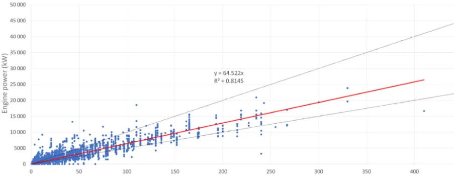
(war-Figure 1.Predicted and actual main engine masses of 31 500 four-stroke engines. The black lines represent the range given by Watson (1998). The red line indicates the mass/power dependency used in this study for cases where engine mass could not be determined.
ships), or for the purpose of not disturbing test subjects (re-search vessels) (Leaper et al., 2014).
Modelling underwater noise from ships has been carried out for a long period of time, and various models have been designed to describe noise sources based on measurements made since the Second World War. However, these models often rely on confidential data sets, which are not necessarily available for civilian research efforts. Nevertheless, over the last two decades significant effort has been made to generate an experimental basis for noise model development (Arve-son and Vendittis, 2000; Kipple, 2002; McKenna et al., 2012; Wales and Heitmeyer, 2002). These data have been used to construct noise source models, which rely on a parametric description of ensemble source spectra for merchant vessels. Recently, Wittekind (2014) described noise sources using a method that presents ships as individual sources of noise which arise from individual technical features and vessel op-eration.
Automatic Identification System (AIS) data have been used to track exhaust emissions from ship traffic, but their use in underwater noise source modelling has only been the sub-ject of few studies where they have mostly been used to lo-cate noise sources relative to hydrophone setups (Hatch et al., 2008; McKenna et al., 2012). Our study extends on this idea and builds on the development of the Ship Traffic Emission Assessment Model (STEAM; Jalkanen et al., 2009, 2012; Jo-hansson et al., 2013, 2017). This approach combines the ves-sel level technical description, an existing noise source model (Wittekind, 2014) and ship activity obtained from AIS data; furthermore, it facilitates the regular updates of noise source maps of any level, ranging from local to global, depending on the availability of AIS data. These data could be used to assess shipping noise, further the understanding of noise as an environmental stressor and provide tools for future sus-tainable governance of marine areas.
The aim of this paper is to (a) introduce a methodology for noise source mapping, which could be used for routine annual reporting of underwater noise emissions, (b) provide insight into the geographical distribution of vessel noise in the Baltic Sea region and (c) provide a summary of results for noise emissions from Baltic Sea shipping during 2015.
2 Materials and methods
2.1 Ship Traffic Emission Assessment Model
of instantaneous engine power, fuel consumption and emis-sions as a function of vessel speed. Further details regarding the model can be found in a recent paper by Johansson et al. (2017).
2.2 Wittekind noise source model
The Wittekind noise source model describes ship noise as a combination of three contributions, which arise from low-and high-frequency cavitation low-and machinery noise. These noise sources are linked to vessel properties, such as dis-placement, hull shape and machinery specifications, which is in contrast with some previously introduced ship noise models (McKenna et al., 2012; Wales and Heitmeyer, 2002). The cavitation contributions are dependent on vessel speed, whereas the machinery contribution is not. This has impor-tant implications for the noise source map generation and the time integration components of this work, which will be de-scribed in Sect. 2.6. The three components are dede-scribed by Wittekind as
SL(fk)=10log10
10SL1(fk)/10+10SL2(fk)/10 (1) +10SL3(fk)/10.
In Eq. (1)fk is the centre frequency of thekth frequency band. The SL1 (Eq. 2) represents the low-frequency cavita-tion noise, the second contribucavita-tion (SL2; Eq. 3) describes the high-frequency cavitation noise and the third (SL3; Eq. 3) represents the machinery noise. In the Wittekind model, the low-frequency cavitation noise (SL1) was obtained from fit-ting to experimental data (Arveson and Vendittis, 2000):
SL1(fk) (fk)= 5
X
n=0
cnfn+80log10
4c BV Vcis (2) +20 3 log10
∇
∇Ref
SL2(fk)= −5 lnf− 1000
f +10+
20 3 log10
∇
∇Ref (3)
+60log101000cBV
Vcis
SL3(fk)=10−7f−0.01f+140+15log10m (4) +10log10n+E.
In Eq. (2),fdenotes the centre frequency of thekth octave band;c0=125,c1=0.35,c2= −8×10⁻³, c3=6×10⁻⁵, c4= −2×10⁻⁷andc5=2.2×10⁻¹⁰are constants;CB de-notes the block coefficient (hull form fullness when com-pared to a rectangular box of same length, width and depth as the ship);V indicates the instantaneous vessel speed obtained from AIS;Vcrepresents the cavitation inception speed;∇ is the vessel displacement; and∇Refis the reference vessel dis-placement, which is 10 000 t. In Eq. (4), the parametersmand
nrepresent the mass (in tonnes) and the number of operat-ing main engines, respectively, andEis the engine mounting parameter which indicates whether the engine is resiliently (E=0) or rigidly (E=15) mounted.
As can be seen, the Wittekind model uses parameters that are ship specific and which lead to individual noise source descriptions depending on vessel features; however, some of these parameters are not available from the ship databases that provide other vessel specifications. Nevertheless, there are numerous parameters that need to be derived during the noise source calculations. Some of these, such ascB,∇andn, are already calculated during a regular STEAM run, but en-gine mass (m), mounting parameter (E) and cavitation incep-tion speed (VCIS) were determined as described in Sect. 2.3, 2.4 and 2.5.
2.3 Main engine mass
Main engine mass is not routinely included in commercial ship databases; therefore, we have augmented the STEAM database with engine masses obtained from technical docu-mentation from engine manufacturers and engine catalogues (Barnes et al., 2005). Engine mass could be explicitly de-termined for about two-thirds of the global fleet. For the third, a linear function was developed to estimate the en-gine mass based on the size (installed power) of enen-gines. For four-stroke engines, the main engine mass was determined by multiplying the installed kW / engine by 0.0155 which cor-responds to a 65 kW t−1power/mass ratio and falls within the range of values proposed by Watson (1998). Cylinder ar-rangement (in-line vs.V arrangement) also has an impact on the predicted mass, as in-line engines tend to be heavier than
V engines; this leads to a lower power / mass correlation than for two-stroke engines. Cylinder arrangement does not apply to two-stroke engines, because only in-line engines are used. There were about 19 600 vessels equipped with four-stroke engines in this study, the mass of which was evaluated with the proposed power / mass methodology. The quality of the linear fit is slightly worse for four-stroke engines (R2= 0.814) than for two-stroke engines (R2=0.955) due to the variable cylinder arrangement described above. There were 24 300 vessels with two-stroke engines, the mass of which could be determined from manufacturer documentation. The mass of two-stroke main engines for 5500 ships needed to be estimated based on the installed engine power (in kW). Further, there were 3100 vessels for which the engine stroke type was unknown. In unknown cases, the most similar ves-sel details (Johansson et al., 2017) were used to determine the missing technical data.
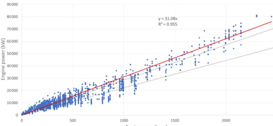
Figure 2.Predicted and actual main engine masses of 24 000 two-stroke engines. The black lines represent the range given by Watson (1998). The red line indicates the mass / power dependency used in this study.
noted that the range recommended by Watson (1998) leads to higher engine masses than the best fit to the engine setup of the current fleet of 24 300 samples.
For gas turbine machinery, 0.001 t kW−1 should be used according to Watson. There are 480 entries in the ship database that indicate the use of turbine machinery, either gas or steam versions. The accuracy of mass predictions for ves-sels equipped with turbine machinery is poor. No correlation was found between the engine mass and the power output. The Watson recommendation was adopted and 0.001 t kW−1 was used for all turbine machinery. It should be noted that the applicability of the Wittekind noise source model to tur-bine machinery is an extrapolation of the original results and is likely to result in large uncertainties.
2.4 Engine mounting
Unfortunately, an engine mounting parameter is not avail-able in the existing technical databases. The main engines of a ship can be bolted directly to the rigid box girder without additional damping material to absorb vibrations of engines. This is known as rigid mounting and is usually applied to large two-stroke engines, but it can also be used for some large four-stroke engines. Resilient mounting of the engine, in comparison, is used if it is necessary to reduce structure-borne vibrations or noise that would otherwise be transmitted to the hull. According to Rowen (2003) and Kuiken (2008), resilient mounting is usually applied to medium- and high-speed diesels, which are sufficiently rigid with respect to bending and torsion. In this work, all two-stroke engines have been assigned a “rigid mounting” status, whilst “resilient mounting” is assumed for all four-stroke engines, although, as previously stated, some four-stroke engines can be
in-stalled using either method (Wartsila, 2012, 2015 2016). We investigated the impact of these assignments on the emitted noise levels from several kinds of ships. Source level curves for some of these cases can be found in Supplement. 2.5 Cavitation inception speed
The description of cavitation is, among other factors, a func-tion of the propeller disc area and the propeller tip speed. The commercial ship databases do not contain enough infor-mation regarding propellers installed on ships, such as the number of blades and diameter, to generate the cavitation inception speed. An alternative method of determining this parameter has consequently been developed founded on dis-cussions with a manufacturer of propulsion equipment. Fol-lowing these discussions, an approach based on the vessel block coefficient and design speed was developed (Eq. 5):
2010). Therefore, if low noise emissions are not considered as a meaningful parameter during the design phase, the grad-ually tightening energy efficiency requirements for ships may lead to ships that are actually noisier than their predecessors. In addition, highly efficient propellers may not be the quietest ones.
2.6 Noise source map generation
To represent underwater noise emissions as a map, an ap-proach was developed to facilitate this form of emission re-porting. The source level is related to the power emitted (Pk) in the frequency bandk, as follows:
SLkdB re 1 m,1 µPa=10log10 Pk
PRef
, (6)
where PRef= 4π p2
ref
ρc is a reference power,ρ and c are the density and speed of sound, respectively, whilepref=1 µPa. Assuming that all noise sources are uncorrelated, the total emitted power from allMships in areaAat timet is given as
Pktot(t )= M
X
m=1
Pk,m(t ), (7)
wherePk,m(t) is the sound power (in J s−1) emitted by ship
m. This quantity is additive and facilitates the summation of ship specific noise energy over a specific period (in joules). The sound power map is more of a visual aid than a direct input data set for noise propagation modelling, which usu-ally demands point source descriptions of the noise sources. For examples of propagation modelling from multiple ships, which facilitates the evaluation of the sound pressure level at an arbitrary point in the water column, the reader is referred to e.g. Karasalo et al. (2017) and Gaggero et al. (2015). Pre-senting sound energy as a geographically distributed quantity will help to visualize noisy areas, as has also been investi-gated by Audoly et al. (2015). Similar to the emission maps of atmospheric pollutants, noise source maps should not be taken as a representative description of underwater noise any more than an emission map of NOx is able to fully describe airborne pollutant concentrations. The maps presented in this work describe the noise sources, not the underwater propaga-tion of noise. It should be noted that the numbers presented as a map are a function of grid cell area and should be nor-malized to unit area. In this work we have used one square kilometre as the grid cell size.
Ships spend a significant portion of their active time in har-bour areas (Smith et al., 2014). The time integration step in this study (Eq. 7) leads to a situation where harbour areas are represented as significant sources of underwater noise. This is a feature of the machinery contribution of the noise source description (see Eq. 4) which remains non-zero when ships are standing still. Using the current approach it is not possi-ble to distinguish between ships standing still with engines
on or off. The Wittekind noise source model is intended for moving vessels and the application of this model to stationary vessels would have been a clear extrapolation of the original intention. For this reason, we chose to only apply the time in-tegration of sound power to moving ships. In STEAM, time integration of sound power is only applied to the cruising and manoeuvring modes of vessel operation, and stationary vessels do not contribute to total sound energy regardless of the fact that there may be auxiliary engines running during harbour visits which may contribute to the emitted underwa-ter noise. Noise from auxiliary engines is not modelled in this approach even if it may be a significant source of atmo-spheric noise in harbour areas. Based on these definitions, a source emitting 1 MJ of noise in 1 year corresponds to a continuous monopole source with an approximate 156 dB re 1 µPa at 1 m sound pressure level, assuming that free-field approximation is valid.
3 Results and discussion
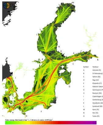
3.1 Shipping noise emissions in the Baltic Sea region The noise maps were generated for one-third octave bands which have 63, 125 and 2000 Hz central frequencies (Van der Graaf et al., 2012). The two lowest bands are relevant for various fish species, whereas the 2 kHz band is relevant for marine mammals (Nedwell et al., 2004; Nikopouloulos et al., 2016). Using the methodology described above, the noise source maps generated for Baltic Sea shipping in 2015 (for 63 Hz band) are depicted in Fig. 3.
As can be seen from Fig. 3 noise source maps have noise hotspots on the main shipping lane in the Danish straits, be-tween the islands of Fyn and Sjælland. Furthermore, high sound energy values were estimated outside Kiel and Ros-tock harbours. The annual noise energy emitted in the 63 Hz band was 117 GJ during 2015, with the highest contribu-tions from bulk cargo ships, container ships and tankers. Noise emissions were also observed to increase towards the end of 2015. Maximum monthly noise energy emissions were noted in December 2015, 32 GJ month−1, whereas the minimum was found to occur in February, 25 GJ month−1. These are summed energies over all three bands, 63, 125 and 2000 Hz. Daily noise energy emissions in January were 0.86 GJ day−1, although emissions exceed 1 GJ day−1 to-wards the end of 2015 (the daily maximum occurred in Oc-tober, 1.07 GJ day−1). These results indicate a 20 % growth in noise energy emissions (in GJ, not dB) during 2015.
Figure 3.Noise source map for Baltic Sea shipping. This map indicates the sum of sound energy in units of joules per grid cell (cell area 1 km2) during the year 2015.
emissions, but bulk carriers represent a larger share of the to-tal number of ships (8 %). (Fig. 4; Table 1). Analogous to energy efficiency metrics, reported in grams of CO2 emit-ted per amount of cargo carried and distance travelled (in g t−1km−1), the emitted noise energy should also be com-pared to transport work or distance travelled. If calculated this way, container ships represent 15 % of the transport work and emit 23 % of the noise energy (the sum of noise en-ergy emitted in the 63, 125 and 2000 Hz bands). Regarding bulk cargo ships, the share of the noise energy emissions is 23 % and the share of the transport work carried out is 21 %. Considering the large share of the transport work, bulk and general cargo ships emit less noise than container ships. The largest discrepancies between noise energy emitted and dis-tance travelled occur with RoPax vessels, which are
respon-sible for 3 % of the transport work and contribute 9 % of the noise energy (the sum of energy over all three bands) emitted in the Baltic Sea region. If the noise efficiency index is de-fined as joules of noise energy emitted for each ton kilometre of cargo carried, the noise efficiency index in mJ t−1km−1is very high for RoPax vessels (920 mJ t−1km−1), whereas for container ships and bulk carriers the noise efficiency indexes is 491 and 360 mJ t−1km−1, respectively. With this metrics, lowest index is achieved with slow moving vessels, like gen-eral cargo carriers and crude oil tankers, which emit less than 200 mJ of noise energy per ton kilometre carried.
Table 1.Noise energy emitted by various ship types in the Baltic Sea region during the year 2015. The top 10 contributors are re-ported and represent over 90 % of the noise energy emitted.
Type Noise energy Noise energy Noise energy
(GJ a−1), (GJ a−1), (GJ a−1),
63 Hz 125 Hz 2000 Hz
Bulk cargo 48.4 24.2 0.4
Container ships 43.7 26.9 0.4
Other tankers 4.9 1.5 0.0
RoRo 13.2 4.3 0.1
RoPax 17.1 11.3 0.2
General cargo 15.0 7.3 0.1
Vehicle carriers 0.6 0.3 0.0
Product tankers 9.0 2.4 0.0
Chemical tankers 38.3 15.7 0.3
Crude oil tankers 27.3 7.8 0.1
Total 237.4 116.6 1.7
fleet in the Baltic Sea region returns to normal operation at speeds closer to ship’s respective design speeds, it is very likely that a significant increase in noise energy will be seen for the quarter of the cargo fleet now operating below their
VCIS. This increase could happen without increasing the fleet size at all. A significant portion of oil product tankers and cruise vessels were also found to be operating at speeds lower than their cavitation inception speed. It may very well be that the contribution from the oil tanker fleet may increase when the vessels that are currently operating below their de-sign speed increase speed, although their overall contribu-tion to sound power is quite low, only about 2 %. However, if the 20 % of container ships which operated under theirVCIS in 2015 speed up, the resulting sound energy increase im-pact will be significant, as the container ship contribution to overall sound power is high. Voluntary speed reduction was also observed in the “Third IMO Greenhouse Gas Study” (Smith et al., 2014), especially in the container ship class. Speed reduction may occur in situations where vessels may not be fully loaded, when overcapacity in the market exists and when the costs can be lowered by sailing slower than the design speed. The required power and the fuel consumption are cubic functions of speed, and speed reductions may lead to significant savings if vessel schedules allow for them. 3.2 Uncertainty evaluation
Karasalo et al. (2017) tested the performance of the Wit-tekind noise source model using inverse modelling from hydrophone measurements. The transmission loss of the measured noise signature was modelled using XFEM code (Karasalo, 1994) to obtain the noise source at a reference dis-tance. In their paper, Karasalo et al. (2017) observed a good fit between the Wittekind predictions and the observed sig-nals for cargo ships, tankers and tugboats, but larger differ-ences were observed for passenger and RoRo vessels, with
the Wittekind model overestimating the noise source levels. It is very likely that this is because the Wittekind model was mainly intended for large ocean-going vessels with a single fixed pitch propeller or a single controllable pitch propeller that are operated close to their design pitch (Dietrich Wit-tekind, personal communication, October 2017).
The voluntary operation of a vessel at lower speeds (slow steaming) may work as a noise mitigation option for deep ocean vessels with a single fixed pitch propeller; however, this method may not be effective for ships equipped with controllable pitch (CP) propellers and may actually lead to higher than expected noise emissions (Wittekind, 2009).
Significant uncertainty may be involved in the estimation of the cavitation inception speed (VCIS), which is not read-ily available directly from any of the ship databases and was estimated in this study using the vessel design speed and hull form (see Eq. 5). The contribution ofVCIS to the ves-sel noise source level is significant, because at speeds below this threshold value vessel noise is notably lower. We tested the impact ofVCIS uncertainty by testing the sensitivity of predicted noise toVCIS; this was done by altering the lower and upper bounds of Eq. (5) to 10 and 15 knots, respectively. This change increased the speed at which the propellers cavi-tated and, therefore, led to larger portion of the fleet operating under non-cavitating conditions than the default assumption. The differences in the predicted noise energy in the Baltic Sea region were most pronounced in the low-frequency band (63 Hz), where the total noise energy emitted decreased by 26 % when higher values ofVCIS were applied. For all fre-quency bands considered, the total reduction was 19 %. The sum of the energy emitted at higher frequency bands also de-creased by 7 % for both the 125 and 2000 Hz bands, respec-tively. The change in the cavitation speed range only altered the noise energy emissions from RoPax ships by 7 %, whilst the results for passenger cruise vessels were unchanged. This is probably because RoPax and cruise vessels mostly oper-ate at speeds faster than 15 knots, and cavitation still oc-curs regardless of the higherVCIStested here. For container ships, noise emissions were reduced by 19 %, but the largest changes (−39 %) occurred in the tanker class. Contributions from other slow moving vessels, like cargo ships, were also significantly reduced (−27 %).
.
Figure 4.Contribution of different ship types to annual emissions of underwater noise energy (share of energy emitted in the 63, 125 and 2000 Hz bands). The dark blue bar represents the share of the specific ship types with respect to all ships included in the study; orange represents the share of transport work; grey, yellow and light blue represent the share of noise energy emitted by ships in the 63, 125 and 2000 Hz bands, respectively with respect to the total energy
Figure 5.Noise energy emitted by different ship types in 125 Hz frequency band (in joules per year; blue bars, left axis). The share of the fleet operating under their cavitation inception speed is also indicated (orange bars, right axis). For example, container ships are the biggest source of noise energy in the Baltic Sea fleet with 27 GJ, of sound power emitted. Of the container ship fleet, about 20 % operate at speeds lower than their predicted cavitation inception speed.
or more propellers, and the contribution of these ship types to the total noise energy in the 125 Hz frequency band was around 13 %. It is likely that the accuracy of the noise emis-sion estimations for the passenger vessel fleet is worse than that of the cargo ships, but this does not change the main conclusions of this paper.
The Wittekind model was built for vessels with a single propeller and a four-stroke main engine. The application of the Wittekind model to large two-stroke engines, which com-monly propel the global fleet, may lead to increased
estimate as the current approach is not able to distinguish be-tween ships anchored with their engines shut down and ships anchored with their engines running. It is very likely that har-bour areas are not significant fish or marine mammal habitats, which should reduce the significance of this uncertainty con-cerning the consequent noise impact assessments on marine life.
4 Summary
Underwater noise is rarely a design parameter for new ships, unless warships or research vessels are considered, and only voluntary guidelines to mitigate vessel noise exist. Currently, for the commercial fleet, the efficiency of the propeller is more important than low noise emissions, and these two con-flicting requirements may lead to worse noise problems in the future when more energy efficient designs are required. Cavitation of propellers is usually avoided to alleviate me-chanical problems arising from erosion, not to mitigate noise emissions.
A methodology was presented to derive underwater noise emissions from ship activity and technical data. This facili-tates annual updates of noise source maps for the 63, 125 and 2000 Hz frequency bands regardless of the study scale. With global AIS data, global noise source studies are also possible. During 2015 the most significant noise sources in the Baltic Sea were bulk carriers and container ships. Container vessels represented about 3 % of the total number of IMO registered vessels, but were responsible for one-quarter of the noise energy emitted; this makes them the largest contributor to vessel noise in the Baltic Sea region. It was discovered that about 20 % of container ships currently operate at speeds be-low the estimated cavitation inception speed. If these vessels were to increase their operating speed to levels closer to their design speed, a significant increase in underwater noise may occur in the Baltic Sea region without any increase in the fleet size. However, the container ship share of the total transport work is almost as large as the container ship noise contribu-tion. Considering the distances travelled and cargo carried, RoPax vessels have a disproportionally large contribution to vessel noise. It is unclear how well the current approach can be applied in multi-propeller, multi-engine cases for which the Wittekind noise model was not originally intended. Fur-ther work is needed to understand the performance of current noise modelling tools in these cases.
It is unclear what kind of physical impact the current level of shipping noise has on marine life in the Baltic Sea. Ship-ping is only one source of underwater noise and many other sources exist, both natural and anthropogenic. Noise is not routinely monitored, but it is measured in many research projects concentrating on underwater noise. There are no long-term observations of noise that could be used to deter-mine how noise levels have developed in the Baltic Sea in the past, but AIS data are available for at least the last decade.
This allows for noise modelling studies covering this period. In general, modelling must rely on robust experimental data, which should be available to assess the performance of the modelling work. Currently, only limited opportunities to do this exist from a handful of research projects; therefore, na-tional measurement networks and internana-tional cooperation are needed.
Data availability. The noise source emission maps in netcdf format are available in the Data Dryad service: https://doi.org/10.5061/dryad.nt22g30.
Supplement. The supplement related to this article is available online at: https://doi.org/10.5194/os-14-1373-2018-supplement.
Author contributions. JPJ was responsible for the overall coordina-tion of the work, the Wittekind noise model adaptacoordina-tion for STEAM and was the main contributor to this paper. LJ was responsible for the technical implementation of the noise module and for running the STEAM model. ML and RB provided technical expertise re-garding the noise model selection and adaptation. PS, MÖ, IK and MA were responsible for developing a methodology for the noise source mapping and the consecutive noise propagation modelling, which contributed to the uncertainty evaluation. HP and JP provided expertise on the relevant impacts of noise on marine life and con-tributed to noise source mapping method development.
Competing interests. The authors declare that they have no conflict of interest.
Special issue statement. This article is part of the special issue “Shipping and the Environment – From Regional to Global Perspec-tives (ACP/OS inter-journal SI)”. It is a result of the Shipping and the Environment – From Regional to Global Perspectives, Gothen-burg, Sweden, 23–24 October 2017.
Acknowledgements. This work resulted from the BONUS SHEBA project and was supported by BONUS (Art 185), which is jointly funded by the EU, the Academy of Finland, the Swedish Agency for Marine and Water Management, the Swedish Environmental Protection Agency and FORMAS. We are grateful to the HELCOM member states for allowing the use of HELCOM AIS data in this research.
Edited by: John M. Huthnance
European Parliament and Council of the European Union: Directive 2008/56/EC of the European Parliament and of the Council, Off. J. Eur. Union, 164, 19–40, https://doi.org/10.1016/j.biocon.2008.10.006, 2008.
Gaggero, T., Rizzuto, E., Karasalo, I., Östberg, M., Folegot, T., Six, L., van der Schaar, M., and Andre, M.: Validation of a simulation tool for ship traffic noise, in Oceans’15, IEEE, 2015.
Hatch, L., Clark, C., Merrick, R., Van Parijs, S., Ponirakis, D., Schwehr, K., Thompson, M., and Wiley, D.: Characterizing the relative contributions of large vessels to total ocean noise fields: A case study using the Gerry E. studds stellwagen bank national marine sanctuary, Environ. Manage., 42, 735–752, https://doi.org/10.1007/s00267-008-9169-4, 2008.
Hildebrand, J.: Sources of Anthropogenic Sound in the Marine Environment, Rep. to Policy Sound Mar. Mamm. An Int. Work. US Mar. Mammal Comm. Jt. Nat. Conserv. Comm. UK London Engl., 50, 1–16, https://doi.org/10.1016/j.marpolbul.2004.11.041, 2004. Hildebrand, J. A.: Anthropogenic and natural sources of
am-bient noise in the ocean, Mar. Ecol. Prog. Ser., 395, 5–20, https://doi.org/10.3354/meps08353, 2009.
IHS_Global: SeaWeb database of the global ship fleet, SEAWEB data product, IHS Fairplay, 2016.
IMO: 2014 GUIDELINES ON THE METHOD OF CALCULA-TION OF THE ATTAINED ENERGY EFFICIENCY DESIGN INDEX (EEDI) FOR NEW SHIPS, International Maritime Or-ganization, 66th meeting of the Marine Environment Protection Committee (IMO MEPC), MEPC 66/21/Add. 1, IMO headquar-ters in London, April 2014.
IMO SDC: PROVISIONS FOR REDUCTION OF NOISE FROM COMMERCIAL SHIPPING AND ITS ADVERSE IMPACTS ON MARINE LIFE, International Maritime Organization, 57th meeting of the Sub-Committee on Ship Design and Construction (DE57), DE 57/17, IMO headquaters in London, March 2013. Jalkanen, J.-P., Brink, A., Kalli, J., Pettersson, H., Kukkonen, J.,
and Stipa, T.: A modelling system for the exhaust emissions of marine traffic and its application in the Baltic Sea area, Atmos. Chem. Phys., 9, 9209–9223, https://doi.org/10.5194/acp-9-9209-2009, 2009.
Jalkanen, J.-P., Johansson, L., Kukkonen, J., Brink, A., Kalli, J., and Stipa, T.: Extension of an assessment model of ship traffic ex-haust emissions for particulate matter and carbon monoxide, At-mos. Chem. Phys., 12, 2641–2659, https://doi.org/10.5194/acp-12-2641-2012, 2012.
tic noise, NSWC Rep., (NSWCCD-71-TR-2002/574), avail-able at: http://www.nps.gov/glba/naturescience/whale_acoustic_ reports.htm#Acoustic (last access: 19 October 2018), 2002. Kuiken, K.: Diesel engines for ship propulsion and power plants-I,
Target Global Energy Training, Onnen, the Netherlands, 2008. Leaper, R., Renilson, M., and Ryan, C.: Shhh ... do you hear that?,
J. Ocean Technol., 9, 50–69, 2014.
McKenna, M. F., Ross, D., Wiggins, S. M., and Hilde-brand, J. A.: Underwater radiated noise from modern commercial ships, J. Acoust. Soc. Am., 131, 92–103, https://doi.org/10.1121/1.3664100, 2012.
Moore, S. E., Reeves, R. R., Southall, B. L., Ragen, T. J., Suy-dam, R. S., and Clark, C. W.: A New Framework for As-sessing the Effects of Anthropogenic Sound on Marine Mam-mals in a Rapidly Changing Arctic, Bioscience, 62, 289–295, https://doi.org/10.1525/bio.2012.62.3.10, 2012.
Nedwell, J. R., Edwards, B., Turnpenny, A. W. H., and Gordon, J.: Fish and Marine Mammal Audiograms?: A summary of avail-able information, Subacoustech Rep. ref 534R0214, (September 2004), 281, 2004.
Nikopouloulos, A., Sigray, P., Andersson, M., and Carlström, J. L. E.: BIAS Implementation Plan – Monitoring and assess-ment guiance for continuous low frequency sound in the Baltic Sea, available at: http://www.diva-portal.org/smash/get/diva2: 1072183/FULLTEXT01.pdf (last access: 19 October 2018), 2016.
Rolland, R. M., Parks, S. E., Hunt, K. E., Castellote, M., Corkeron, P. J., Nowacek, D. P., Wasser, S. K., and Kraus, S. D.: Evidence that ship noise increases stress in right whales, Proc. Biol. Sci., 279, 2363–2368, https://doi.org/10.1098/rspb.2011.2429, 2012. Rowen, A. L.: Chapter 24. Machinery Considerations, in Ship
De-sign & Construction, Vol 1, edited by: Lamb, T., The Society of Naval Architects and Engineers (SNAME), Jersey City, NJ, 2003.
Smith, T. W. P., Jalkanen, J. P., Anderson, B. A., Corbett, J. J., Faber, J., Hanayama, S., O’Keeffe, E., Parker, S., Johansson, L., Aldous, L., Raucci, C., Traut, M., Ettinger, S., Nelissen, D., Lee, D. S., Ng, S., Agrawal, A., Winebrake, J. J., Hoen, M., Chesworth, S., and Pandey, A.: Third IMO GHG Study 2014, International Mar-itime Organisation (IMO) London, UK, June 2014.
Di-rective – Good Environmental Status (MSFD GES): Report of the Technical Subgroup on Underwater noise and other forms of energy, available at: http://ec.europa.eu/environment/marine/pdf/ MSFD_reportTSG_Noise.pdf (last access: 5 November 2018), 2012.
Wales, S. C. and Heitmeyer, R. M.: An ensemble source spectra model for merchant ship-radiated noise, J. Acoust. Soc. Am., 111, 1211–1231, https://doi.org/10.1121/1.1427355, 2002. Wartsila: Wartsila 46DF Product Guide, Technical
doc-umentation for Wartsila 46DF engine, available at: https://cdn.wartsila.com/docs/default-source/product-files/ engines/df-engine/product-guide-o-e-w46df.pdf?sfvrsn=9 (last access: 19 October 2018), 2016.
Wärtsilä: Wärtsilä 50DF Product Guide, Technical doc-umentation for Wartsila 50DF engine, available at: https://cdn.wartsila.com/docs/default-source/product-files/ engines/df-engine/product-guide-o-e-w50df.pdf?sfvrsn=9 (last access: 19 October 2018), 2012.
Wärtsilä: Wärtsilä 32 Product Guide, Technical doc-umentation for Wartsila 32 engine, available at: https://www.wartsila.com/docs/default-source/product-files/ engines/ms-engine/product-guide-o-e-w32.pdf?utm_source= engines&utm_medium=dieselengines&utm_term=w32&utm_ content=productguide&utm_campaign=msleadscoring (last access: 19 October 2018), 2015.
Watson, D. G. M.: Practical Ship Design, in: Elsevier Ocean Engi-neering Series Volume 1, ISBN-13: 978-0080429991, ISBN-10: 0080429998, Elsevier Science, Oxford, UK, 1998.
Wittekind, D.: The Increasing Noise Level in the Sea – a Chal-lenge for Ship Technology?, Paper given at the 104 th Congress of the German Society for Maritime Technology What causes the noise level in the What is the cause of shipping noise?, in 104th Congress of the German Society for Marine Technol-ogy, p. 8, available at: https://www.iqoe.org/sites/default/files/ files/Wittekind.pdf (last access: 19 October 2018), 2009. Wittekind, D. K.: A simple model for the underwater
noise source level of ships, J. Sh. Prod. Des., 30, 1–8, https://doi.org/10.5957/JSPD.30.1.120052, 2014.