TCSC DESIGNED OPTIMAL POWER
FLOW USING GENETIC ALGORITHM
1
G.MadhusudhanaRao, 2Dr.B.V.SankerRam, 3B.Sampath Kumar
1
G.MadhusudhanaRao, Professor in the Department of EEE in KL University, Guntur,AndhraPradesh. 2
Dr.B.V.sankerRam, Professor in the Department of EEE in JNTUH-Hyderabad, AndhraPradesh. 3
Assistant Professor, in the Department of EEE ARJUN CET- Hyderabad, AndhraPradesh
Abstract:This Paper presents the solution of Optimal Power Flow (OPF) with different objective functions i.e. fuel cost minimization and active power loss minimization using heuristic technique namely Genetic Algorithm (GA) .The basic OPF solution is obtained with fuel cost minimization as the objective function and the optimal settings of the power system are determined. For reactive power optimization, active power loss has been taken as the objective function. OPF solution with the Thyristor Controlled Series Compensator [7] device is carried out considering fuel cost minimization and active power loss minimization as objective. TCSC is used to minimize the total fuel cost and active power losses. All the above cases are done by Genetic Algorithm. Results obtained using IEEE 30 bus system and 75-bus Indian system are presented.
Keywords: TCSC, Optimal Power Flow, Genetic Algoritm,Cost minimisaton
1. INTRODUCTION
FACTS devices have opened a new world in power system control. They have made the power systems operation more flexible and secure. They have the ability to control, in a fast and effective manner, the three effective players in power flow. These are circuit impedance, voltage magnitude and phase angle. Gaining flexibility in power flow is not a little achievement. The great economic and technical benefits of this to the power systems have been well proven.Installing FACTS devices in any power system is an investment issue. It offers some flexibility to the power system at the expense of cost.
Therefore, it is necessary for any new installation of FACTS to be very well planned. Planning of FACTS devices manly means the allocation of those devices in the power system. This needs an off-line simulation of the power system with the different candidate FACTS devices location to assess the value added to the system in terms of system operation improvement. Among the different assessment tools used for this purpose, optimal power flow (OPF) [2], [4] seems to be the best. By incorporating FACTS devices [9] in OPF with some modification, it can give scalar measures of its economic and technical benefits and so help in deciding for the optimal investment.OPF is a non-linear problem and can be non-convex in some cases. Moreover, incorporating FACTS devices complicates the problem further. Such complicated problem needs a well-efficient optimization technique for solving. Genetic algorithm is such efficient technique employed for this task in this paper.
2.FACTS MODELING
2.1 Thyristor controlled series compensation (TCSC).
Figure 1. Thyristor controlled series compensation
)
(
)
(
' ' ' ij ij ij ij ij ijij
y
y
g
jb
g
jb
y
2 2 ij ij ij ij x r r g , 2 2 ij ij ij ij x r x b 2 2 ' ) ( ij cij ij ij x x r r g 2 2 '
)
(
ij cij c ij ij
x
x
r
x
x
b
After adding TCSC on the line between bus i and bus j of a general power system, the new system admittance matrix Y’bus can be updated as:
j col i col j row i row y y y y Y Y ij ij ij ij bus bus 0 0 0 ... 0 0 0 0 0 ... 0 0 0 0 0 ... 0 0 0 0 ... 0 ... ... ... ... 0 0 0 ... 0 0 0 0 0 ... 0 0 0 0 0 ... 0 0 0 '
3. PROBLEM FORMULATION
3.1 Problem Variables: Optimal power system operation seeks to optimize the steady state performance of a power system in terms of an objective function while satisfying several equality and inequality constraints. Generally, OPF is formulated an optimization problem as follows:
Minimize
J
(
x
,
u
)
Subject to
g
(
x
,
u
)
0
h
(
x
,
u
)
0
u
: Vector of problem control variablex
: Vector of system state variables)
,
(
x
u
J
: Objective function to be minimized)
,
(
x
u
g
: Equality Constraints [1] represents nonlinear load flow equations.)
,
(
x
u
h
: Inequality Constraints i.e. system functional operating constraints.Where
u
is a vector of control variables consisting of generator voltagesV
G, generator real power outputsP
G except at slack bus1
G
P
, transformer tap settingsT
and shunt VAR compensationQ
c. Henceu
can be expressed as]
...
,
...
,
...
,
...
[
1 21 GNG G GNG 1 NT C CNC
G T
Q
Q
T
T
P
P
V
V
u
3.2. Objective Functions: J is the objective function to be minimize, which is one of the following:
Fuel cost minimization:
It seeks to find the optimal active power outputs of the generation plants so as to minimize the total fuel cost. This can be expressed as
Where fi is the fuel cost curve of the ith generator and it is assumed here to be represented by the following quadratic function:
)
/
($
2
hr
P
c
P
b
a
f
i i i G
G i i
i
Where ai, bi, and ci are the cost coefficients of the ith generator
Active power loss minimization:
The objective function J is considered as active power loss of the system.
nlinei
i
c
x
y
Loss
f
J
1
)
,
(
Where nline is number of branches.
3.3. Problem Constraints
Equality constraints:The equality constraints that are the power flow equations corresponding to both real and reactive power balance equations, which can be written as:
0
)
,
(
P
P
V
P
G D ii i
0
)
,
(
Q
Q
V
Q
Gi Di iWhere
)
sin
cos
(
ij ij ij ij ji
i
V
V
G
B
P
)
sin
cos
(
ij ij ij ijj i
i
V
V
B
G
Q
Inequality constraints:The inequality constraintsare the system operating limits. The inequality constraints that are real power outputs, reactive power outputs and generator outputs.
4.SOLUTION METHODOLOGY 4.1. Over view:
GA is used to solve the OPF problem. The control variables [6] modeled are generator active power out puts, voltage magnitudes, shunt devices, and transformer taps. To keep the GA chromosome size small, each control variable is encoded with different sizes. The continuous control variables include generator active power outputs, generator voltage magnitudes, and discrete control variables include transformer tap settings and switchable shunt devices.
Figure2.GA chromosome structure
4.2. The Proposed GA Algorithm
Typically it consist of three phases, (i) Generation
(ii) Evaluation
(iii) Genetic operation
4.2.1. Generation
4.3. Evaluation
In the evaluation phase, suitability of each of the solutions from the initial set as the solution of the optimization problem is determined. For this function called “fitness function” is defined. This is used as a deterministic tool to evaluate the fitness of each chromosome. The optimization problem may be minimization or maximization type. In the case of maximization type, the fitness function can be a function of variables that bear direct proportionality relationship with the objective function [5]. For minimization type problems, fitness function can be function of variables that bear inverse proportionality relationship with the objective function or can be reciprocal of a function of variables with direct proportionality relation ship with the objective function. In either case, fitness function is so selected that the most fit solution is the nearest to the global optimum point. The programmer of GA is allowed to use any fitness function that adheres to the above requirements. This flexibility with the GA is one of its fortes.
4.4. Genetic operation
In this phase, the objective is the generation of new population from the existing population with the examination of fitness values of chromosomes and application of genetic operators. These genetic operators are reproduction, crossover, and mutation. This phase is carried out if we are not satisfied with the solution obtained earlier. The GA [3] utilizes the notion of survival of the fittest by transferring the highly fit chromosomes to the next generation of strings and combining different strings to explore new search points.
4.4.1. Reproduction
Reproduction is simply an operator where by an old chromosome is copied into a Mating pool according to its fitness value. Highly fit chromosomes receive higher number of copies in the next generation. Copying chromosomes according to their fitness means that the chromosomes with a higher fitness value have higher probability of contributing one or more offspring in the next generation.
4.4.2. Cross over
It is recombination operation. Here the gene information (information in a bit) contained in the two selected parents is utilized in certain fashion to generate two children who bear some of the useful characteristics of parents and expected to be more fit than parents.
Crossover is carried out using any of the following three methods (a)Simple or Single Point Crossover
(b) Multi point crossover (c) Uniform crossover
4.4.3. Mutation
This operator is capable of creation new genetic material in the population to maintain the population diversity. It is nothing but random alteration of a bit value at a particular bit position in the chromosome. The following example illustrates the mutation operation
.
Original String:1011001 Mutation site: 4 (assumption) String after mutation: 1010001
Some programmers prefer to choose random mutation ‘or’ alternate bit mutation. “Mutation Probability (Pm)” is a parameter used to control the mutation. For each string a random number between ‘0’ and ‘1’ is generated and compared with the Pm. if it is less than Pm mutation is performed on the string. Some times mutation is performed bit-by-bit also instead of strings. These results in substantial increase in CPU time but performance of GA will not increase to the recognizable extent [7]. So this is usually not preferred. Thus obviously mutation brings in some points from the regions of search space which otherwise may not be explored. Generally mutation probability will be in the range of 0.001 to 0.01. This concludes the description of Genetic Operators.
5. RESULTS AND DISCUSSIONS
fuel cost minimization as objective
When fuel cost minimization taken as objective, fuel cost will be reduced but active power losses will be increased.
Active power loss minimization as objective
When active power loss minimization taken as objective, active power losses will be reduced but fuel cost will be increased.
To reduce both fuel cost and active power losses, both fuel cost and active power losses taken as objective.
fuel cost and active power loss minimization as objective
If both fuel cost and active power loss minimization taken as objective, both will be reduced.
5.1. Case study (i)-IEEE 30 bus system
The GA parameters are Population size = 40
Maximum number of generations = 100 Elitism probability = 0.15
Cross over probability = 0.95 Mutation probability = 0.001
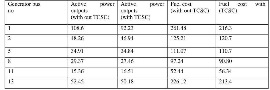
From the analysis of above results, both fuel cost and active power losses taken as objective, due to the influence of TCSC fuel cost reduced from 872.667$/hr to829.40 $/hr, and active power losses are reduced from 5.7255MW to 5.422 MW.
Table 1 OPF results for IEEE 30 bus system with fuel cost and active power loss minimization as objective
Generator bus no
Active power outputs
(with out TCSC)
Active power outputs
(with TCSC)
Fuel cost (with out TCSC)
Fuel cost with (TCSC)
1 108.6 92.23 261.48 216.3
2 48.26 46.94 125.21 120.7
5 34.91 34.84 111.07 110.7
8 29.37 27.46 97.24 90.80
11 15.36 16.51 52.44 56.34
13 52.45 50.18 226.12 213.4
Table 2Pgmax and Pgmin for Generators
Generator bus no Pgmin Pgmax
1 0.5 2.0
2 0.2 0.8
5 0.15 0.5
8 0.1 0.35
11 0.1 0.3
13 0.2 0.8
Table 3 a, b, c constants for generators
1 0 2 0.00375
2 0 1.75 0.0175
3 0 1 0.0625
4 0 3.25 0.002075
5 0 3 0.025
6 0 3 0.025
5.2. Case study (i)-75 bus Indian practical system
GA parameters are: Population size = 40
Maximum number of generations = 100 Elitism probability = 0.15
Cross over probability = 0.95 Mutation probability = 0.001
Fig 3 shows the single line diagram of 75 bus Indian system, and table shows the a.b.c coefficients of 75 bus system.
Figure3. Single line diagram of 75-bus Indian system
Table4.a,b,c coefficients for 75 –bus Indian practical system
Generator bus no
Active power outputs (with out TCSC)
2 1.903 0.805
3 1.633 1.460
4 0.838 1.983
5 0.872 0.987
6 0.941 0.710
7 0.887 0.982
8 5.148 5.443
9 2.306 1.774
10 1.924 1.025
11 2.152 1.937
12 8.520 8.751
13 1.386 1.090
14 3.287 3.472
15 7.841 7.938
Table5.comparision of 75 –bus Indian practical system from the analysis of above results, both fuel cost and active power losses taken as objective, due to the influence of TCSC fuel cost reduced from 8044.8$/hr to7896.7$/hr, and active power losses are reduced from 176.07MW to 155.97 MW.The effect of TCSC in a system will minimize total fuel cost or active power losses or both fuel cost and active power losses.
6. CONCLUSIONS
In this paper Optimal power flow (OPF)[2] has been solved using genetic algorithm (GA) to obtain the optimal fuel cost and active power losses. To reduce the total fuel cost and active power losses further, OPF has been solved with FACTS device like TCSC.
6.1. Case 1: IEEE 30 bus system
Fuel cost minimization taken as objective, due to the influence of TCSC the fuel cost reduced from 849.41$/hr to828.332$/hr.
Active power loss minimization taken as objective, due to the influence of TCSC the active power losses are reduced from 4.3285MW to 3.4925MW.
Both fuel cost and active power losses taken as objective, due to the influence of TCSC fuel cost reduced from 872.667$/hr to829.40 $/hr, and active power losses are reduced from 5.7255MW to 5.422 MW.
6.2 Case 2: 75 bus Indian system
Fuel cost minimization taken as objective, due to the influence of TCSC the fuel cost reduced from 7986.9$/hr 7947.7$/hr.
Active power loss minimization taken as objective, due to the influence of TCSC the active power losses are reduced from 142.73MW to 141.16MW.
Both fuel cost and active power losses taken as objective, due to the influence of TCSC fuel cost reduced from 8044.8$/hr to7896.7$/hr, and active power losses are reduced from 176.07MW to 155.97 MW. From the analysis of above results, the effect of TCSC in a system will minimize total fuel cost or active power losses or both fuel cost and active power losses
[1] Alberto Berrizzi, Maurizio Delfanti, Paolo Marannino, Marco savino pasquadibisceglie, andrea Silvestri, “Enhanced security-constrained OPF with FACTS devices,” IEEEtrans.on power systems, vol.20 no.3, august 2005
[2] M.S.Osman, M.A.Abo-sinna, A.A.Mousa, “A solution to the optimal power flow using genetic algorithm”, Appl.math.comput.2003.
[3] William D.Rosehart, Claudio A canizares,` `Multi objective optimal power flows to evaluate voltage security costs in power net works,” IEEE trans. On power systems, vol.18,no2 ,may2003
[4] Anastasios G. Bakirtzis, Pandel N. Biskas, Christoforos E. Zoumas, Vasilios Petridis, ”Optimal Power Flow by Enhanced Genetic Algorithm,” IEEE Transactions On Power Systems, Vol. 17, no. 2, pp 229-236, May 2002.
[5] X.-P. Zhang and E. Handschin, “Optimal power flow control by converter based facts controllers,” in Proc. 7th Int. Conf. AC-DC Power Transm., London, U.K., pp 28–30, Nov 2001.
[6] L. L. Lai, J. T. Ma, R. Yokoyama, and M. Zhao, “Improved genetic algorithms for optimal power flow under both normal and contingent operation states,” Elec. Power Energy Syst., Vol. 19, no. 5, pp. 287–292, 1997.
[7] M.Noroozian, G.Anderson, “Power Flow Control by Use of Controllable Series components,” IEEE Transactions on Power Delivery, VO1.8, No.3, July 1993, 1420-1428
[8] Rajasekharan, G.A. Vijayalakshmi pai, “Neural Networks, Fuzzy Logic, and Genetic Algorithms Synthesis and Applications”, Prentice-Hall of India Private limited.
[9] Narain G.Hingorani, Laszlo Gyugyi, “Understanding FACTs”, Concepts and technology of Flexible AC Transmission Systems,