Simple statistics for complex Earthquake time distributions

(1)

https://doi.org/10.5194/npg-25-497-2018 © Author(s) 2018. This work is distributed under the Creative Commons Attribution 4.0 License.

Simple statistics for complex Earthquake time distributions

Teimuraz Matcharashvili1, Takahiro Hatano2, Tamaz Chelidze1, and Natalia Zhukova1

1_{M. Nodia Institute of Geophysics, Tbilisi State University, Tbilisi, Georgia} 2_{Earthquake Research Institute, the University of Tokyo, Tokyo, Japan}

Correspondence:Teimuraz Matcharashvili ([email protected]) Received: 24 December 2017 – Discussion started: 19 January 2018 Revised: 4 June 2018 – Accepted: 13 June 2018 – Published: 10 July 2018

Abstract.Here we investigated a statistical feature of quake time distributions in the southern California earth-quake catalog. As a main data analysis tool, we used a simple statistical approach based on the calculation of integral devi-ation times (IDT) from the time distribution of regular mark-ers. The research objective is to define whether and when the process of earthquake time distribution approaches to ran-domness. Effectiveness of the IDT calculation method was tested on the set of simulated color noise data sets with the different extent of regularity, as well as for Poisson process data sets. Standard methods of complex data analysis have also been used, such as power spectrum regression, Lempel and Ziv complexity, and recurrence quantification analysis, as well as multiscale entropy calculations. After testing the IDT calculation method for simulated model data sets, we have analyzed the variation in the extent of regularity in the southern California earthquake catalog. Analysis was carried out for different periods and at different magnitude thresh-olds. It was found that the extent of the order in earthquake time distributions is fluctuating over the catalog. Particularly, we show that in most cases, the process of earthquake time distributions is less random in periods of strong earthquake occurrence compared to periods with relatively decreased lo-cal seismic activity. Also, we noticed that the strongest earth-quakes occur in periods when IDT values increase.

1 Introduction

Time distributions of earthquakes remains one of the impor-tant questions in present-day geophysics. Nowadays, the re-sults of theoretical research and the analysis of features of earthquake temporal distributions from different seismic re-gions with different tectonic regimes carried out worldwide

can be found in Matcharashvili et al. (2000), Telesca et al. (2001, 2012), Corral (2004), Davidsen and Goltz (2004), Martínez et al. (2005), Lennartz et al. (2008), and Chelidze and Matcharashvili (2007).

Such analyses, among others, often aim at the assessment of the strength of correlations or the extent of the determin-ism and/or regularity in the earthquake time distributions. One of the main conclusions of such analyses is that earth-quake generation, in general, does not follow the patterns of a random process. Specifically, well established clustering, at least in time (and spatial domains), suggests that earth-quakes are not completely independent and that seismicity is characterized by slowly decaying correlations (named long-range correlations); such behavior is commonly exhibited by nonlinear dynamical systems far from equilibrium (Peng et al., 1994, 1995). Moreover, it was shown that in the tem-poral and spatial domains, earthquake distributions may re-veal some features of a low-dimensional, nonlinear structure, while in the energy domain (magnitude distribution) distri-butions are close to a random-like, high-dimensional process (Goltz, 1998; Matcharashvili et al., 2000). Moreover, accord-ing to present views, the extent of regularity of the seismic process should vary in time and space (Goltz, 1998; Matcha-rashvili et al., 2000, 2002; Abe and Suzuki, 2004; Chelidze and Matcharashvili, 2007; Iliopoulos et al., 2012).

(2)

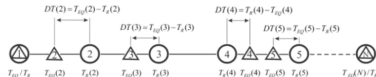
Figure 1.Explanation of the used approach. Triangles – time location of original earthquakes (TEQ(i)), circles – time location of regular

markers (TR(i)). DT(i)denotes the difference between the time of earthquake occurrence (TEQ(i)) in the catalog and the time point of the

regular marker (TR(i)).

2 Data and methods

Our analysis is based on the southern California earthquake catalog available from http://www.isc.ac.uk/iscbulletin/ search/catalogue/ (last access: 5 July 2018). As far as we aimed to analyze temporal features of original earthquake generation, we tried to have a long as possible period of observation with a low-as-possible representative threshold. For this purpose, according to results of time completeness analysis (not shown here), we decided to focus on the time period from 1975 to 2017 since in the middle of the 1970s of the last century the magnitude of completeness clearly decreased. The southern California (SC) earthquake catalog for the considered period is complete forM=2.6, according to the Gutenberg–Richter relationship analysis.

In general, we are presently developing an approach aim-ing to discern features of the complex data sets (in this case earthquake, EQ, time distribution) by comparing them with data sets with the predefined dynamical structures. In the present work, in the frame of this general idea, we started from the simplest case, comparing the natural time distribu-tion of earthquakes in SC catalog with the time distribudistribu-tion of regular markers, according to the scheme shown in Fig. 1. Particularly, knowing the duration of the whole period of observation in the considered catalog (22 167 178 min, from 1 January 1975 to 23 February 2017) and the number of earthquakes (34 020) with the magnitude above a represen-tative threshold (M=2.6), we calculated the time step be-tween consecutive regular markers (651.6 min), which in fact is the mean time of earthquake occurrence for the considered period. Then, for each earthquake in the catalog, we calcu-lated the difference between original event occurrence time and the time point of the regular marker. We denoted DT(i) as the time interval (delay or deviation time) between occur-rence of the original earthquake TEQ(i)and corresponding ith regular marker TR(i). It is clear that the original earth-quake (EQi) may occur prior to or after the corresponding regular marker (Ri), so by DT(i)with minus or plus sign we understand that earthquakes occurred prior to or after regular markers accordingly. More generally, we speak about differ-ences (deviations) between observed waiting timesx(i)and mean occurrence timexover the considered period. It is clear that the character of evolution of these deviations should be

closely related with the character of the considered process, here earthquake time distributions. Thus, alternatively to the above-mentioned text, integral deviation times (IDTs) can be calculated as cumulative sums of deviations. In any case, IDT will depend on the time span of the analyzed period (or the sum of waiting times, as well as on the number of waiting time data,n. Therefore, we calculated norm IDT values for the window span and number of data in analyzed window. It is expected that whenn→ ∞, IDT will approach zero. Log-ically, for a random sequence, the sum of the deviation times should approach zero faster compared to less random ones. This is the main assumption of the present analysis. From this point of view, the approach looks close to the cumulative sums (Cusum) test, where for a random sequence, the sum of excursions of the random walk should be near zero (Rukhin et al., 2010).

Prior to using it for the seismic process, we needed to ful-fill empirical testing of the idea behind the IDT calculation procedure. Specifically, we aimed to test whether the IDT calculation can be sensitive to dynamical changes occurring in complex data sets with known dynamical structures. We started from the analysis of model data sets with a different extent of randomness. Specifically, we used simulated noise data sets of different color with a power spectrum function (1/fβ), where the scale exponent(β)varied from about 0 to 2. These noises, according to generation principles, logi-cally have to be different, but for purposes of our analysis we needed to have strong quantitative assessments of such differ-ences. This is why at first, these noise data sets have been in-vestigated by several data analysis methods, often used to as-sess different aspects of changes occurring in dynamical pro-cesses of interest. Specifically, power spectrum regression, Lempel and Ziv algorithmic complexity calculation, as well as recurrence quantification analysis and multiscale entropy calculation methods have been used for simulated model data sets. All these popular methods of time series analysis are well described in a number of research articles and we will just briefly mention their main principles.

(3)

and the frequency(f )by spectral exponentβ: S(f )∼ 1

fβ, (1)

whereβis often regarded as a measure of the strength of the persistence or anti-persistence in data sets. As easily calcu-lated from the log–log power spectrum plot, β is related to the type of correlations present in the time series (Malamud and Turcotte, 1999; Munoz-Diosdado et al., 2005; Stadnitski, 2012). For example,β=0 corresponds to the uncorrelated white noise, and processes with some extent of memory or long-range correlations are characterized by nonzero values of spectral exponents.

Next, we proceeded to the Lempel and Ziv algorithmic complexity (LZC) calculation (Lempel and Ziv, 1976; Aboy et al., 2006; Hu et al., 2006), which is a common method for quantification of the extent of order (or randomness) in data sets of different origins. LZC is based on the transforma-tion of an analyzed sequence into a new symbolic sequence. For this, original data are converted into a 0, 1, sequence by comparing to a certain threshold value (usually median of the original data set). Once the symbolic sequence is obtained, it is parsed to obtain distinct words, and the words are encoded. Denoting the length of the encoded sequence for those words, the LZC can be defined as

CLZ= L(n)

n , (2)

whereL(n)is the length of the encoded sequence andnis the total length of the sequence (Hu et al., 2006). Parsing methods can be different (Cover and Thomas, 1991; Hu et al., 2006). In this work, we used the scheme described in Hu et al. (2006).

Next, in order to further quantify changes in the dynamical structure of simulated data sets, we have used the recurrence quantification analysis (RQA) approach (Zbilut and Webber, 1992; Webber and Zbilut, 1994; Marwan et al., 2007). RQA is often used for analysis of different types of data sets and represents a quantitative extension of the recurrent plot con-struction method. The recurrent plot itself is based on the fact that returns (recurrence) to the certain condition of the system (or state space location) is a fundamental property of any dynamical system with quantifiable extent of deter-minism in underlying laws (Eckman et al., 1987). In order to successfully fulfill RQA calculations, the phase space tra-jectory should be reconstructed from the given scalar data sets at first. It is important to test the proximity of points of the phase trajectory by the condition that the distance be-tween them is less than a specified threshold ε(Eckman et al., 1987). In this way, we obtain a two-dimensional repre-sentation of the recurrence features of dynamics, which is embedded in a high-dimensional phase space. Then, a small-scale structure of recurrent plots can be quantified (Zbilut and Webber, 1992; Webber and Zbilut, 1994, 2005; Marwan et al., 2007; Webber et al., 2009; Webber and Marwan, 2015).

Particularly, the RQA method enables us to quantify features of a distance matrix of recurrence plot, by means of several measures of complexity. These measures of complexity are based on the quantification of diagonally and vertically ori-ented lines in the recurrence plot. In this research, we cal-culated one such measure: the percent determinism (%DET) which is defined as the fraction of recurrence points that form diagonal lines of recurrence plots and which shows changes in the extent of determinism in the analyzed data sets.

An additional test, which we used to quantify the extent of regularity in the modeled data sets, is the composite multi-scale entropy (CMSE) calculation (Wu et al., 2013a). The CMSE method represents expansion of the multiscale en-tropy (MSE) (Costa et al., 2015) method, which in turn orig-inates from the concept of sample entropy (SampEn; Rich-man and MoorRich-man, 2000). SampEn is regarded as an estima-tor of complexity of data sets for a single timescale. In order to capture the long-term structures in the time series, Costa et al. (2015) proposed the above-mentioned MSE algorithm, which uses SampEn of a time series at multiple scales. At the first step of this algorithm, often used in different fields, a coarse-graining procedure is used to derive the represen-tations of a system’s dynamics at different timescales; at the next step, the SampEn algorithm is used to quantify the regu-larity of a coarse-grained time series at each timescale factor. The main problem of MSE is that, for a shorter time series, the variance in the entropy estimator grows very fast as the number of data points is reduced. In order to avoid this prob-lem and reduce the variance of estimated entropy values at large scales, the method of the CMSE calculation was devel-oped by Wu and colleagues (Wu et al., 2013a).

3 Results and discussion 3.1 Analysis of model data sets

(4)

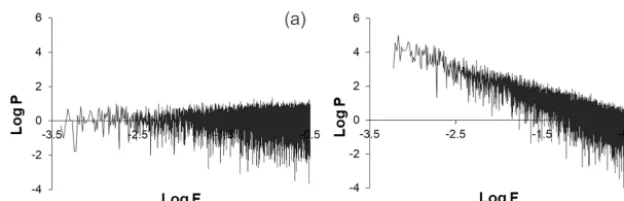
Figure 2.Typical plot of the power spectrum of simulated data sets with different spectral regressions,(a)β=0.001 and(b)β=1.655.

analyzed seven such data sets having the following spec-tral exponents: 0.001, 0.275, 0.545, 0.810, 1.120, 1.387, and 1.655. Values ofβ are often used as a metric for the fractal characteristics of data sequences (Shlesinger, 1987; Schae-fer et al., 2014). In our case, difSchae-ferent spectrum exponents of simulated noise data sets indicate that they are different by the extent of correlations in the frequency content (Schae-fer et al., 2014). Indeed, the first noise set, withβ=0.001 (Fig. 2a) was closest to the white noise and the last one, withβ=1.655 (Fig. 2b), manifested the features closer to colored noises of red or Brownian type, with detectable dy-namic structure. In addition to this, taking into account that we aimed to analyze seismic data sets, we regarded it logi-cal to also consider the random process, which is often used by seismologists – a Poisson process. We generated the set of 34 020 data-long sequences of the Poisson process. It was quite expected that the spectral exponent of such sequences is close to that of white noise.

For further analysis, in order to differentiate simulated (noise and Poisson process) data sets by the extent of ran-domness, we used algorithmic complexity (LZC) and re-currence quantification analysis methods, as well as testing based on MSE analysis.

In Fig. 3, we show results of LZC and %DET calculations; particularly presented here are averages of values calculated for consecutive 1000 data windows shifted by 100 data. Both methods, though based on different principles, help to an-swer the question of how similar or dissimilar the consid-ered data sets are by the extent of randomness. We see that the Lempel and Ziv complexity measure decreases from 0.98 to 0.21 whenβ of noises increases. This means that the ex-tent of regularity in simulated data sets increases. The same conclusion is drawn from RQA: the percentage of determin-ism increases from 25 to 96.5 when the spectral exponent increases. For both LZC and RQA measures, differences in compared neighbor groups in figures are statistically signifi-cant atp=0.01. Thus, according to Fig. 3, the extent of reg-ularity in simulated noise sequences clearly increases from close to white (β=0.001) to close to Brownian (β=1.655) noise. For the Poisson process data sequences, the LZC mea-sure reaches 0.97–0.98 and %DET is in the range 25–26, i.e., these values are close to what we obtain for white noise.

Thus, the results of LZC and %DET calculations confirm the result of power spectrum exponent calculations, and show that considered color noise data sets are different from white noise and the Poisson process by the extent of regularity.

Additional multiscale, CMSE, analysis also shows (Fig. 4) that the extent of regularity in model noise data sets in-creases, when they become “more” colored (fromβ=0.001 toβ=1.655). We see that for small scales (exactly for scale one and partly scale two), noise data sets reveal decreases in the entropy values for simulated data sets, when spectral indexes rise from β=0.001 to β=1.655. This is logical for simulated data sets, where the extent of order, according to the above analysis, should slightly increase. At the same time, while at larger scales, the value of entropy for the noise data set withβ=0.001 continues to monotonically decrease like for the coarse-grained white noise time series (Costa et al., 2015). On the other hand, the value of entropy for 1/f type processes with theβ values close to pink noise (0.81, 1.12) remained almost constant for all scales. As noticed by Costa et al. (2015), this fact was confirmed in different arti-cles on multiscale entropy calculation (see e.g., Chou, 2012; Wu et al., 2013a, b). Costa and coauthors explained this result by the presence of complex structures across multiple scales for 1/f type of noises. From this point of view, in a color noise set closer to a Brownian-type process, the emerging complex dynamical structures should become more and more organized. Apparently, these structures are preserved over multiple scales including small ones. This is clearly indicated by the gradual decrease in calculated values of entropy for sequences withβ=1.12 toβ=1.387 andβ=1.654 at all considered scales (see Fig. 4). Poisson process data sets (not shown in figure) in the sense of results of multiscale analysis are close to a white noise sequence withβ=0.001.

Thus, CMSE analysis additionally confirms that the com-plex model data sets used in this research are characterized by quantifiable dynamical differences.

Once we had data sets with quantifiable differences in their dynamical structures, we started to test the ability of the IDT calculation to detect these differences.

(5)

oc-Figure 3.LZC and %DET values calculated for seven noise data sets with different spectral indexes.

Figure 4.CMSE values versus scale factor for simulated data se-quences with different spectral indexes.

currence sequence of real earthquakes and calculated IDT values for different windows. Taking into consideration that cumulative sum (or time span in the case of seismic catalog) of windows may be different (excluding the case when data sets have been specially generated so that the cumulative sum is equal) we obtained normed IDT values to the span of win-dow and the number of data. Results of the calculation are presented in the lower curve (circles) in Fig. 5a. Here also we present results of similar calculations on the same data sets performed for shorter windows (see squares, triangles, and diamonds in Fig. 5a).

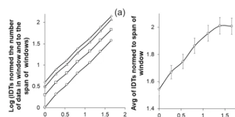
As we see, absolute values of IDTs normed to window span and number of data, calculated for the model data sets, indicate stronger deviation from zero, when the extent of or-der in simulated noise data sets increases (according to the above analysis). Average values of IDTs calculated for data sets with spectral exponents closer to Brownian noise signif-icantly differ from white noise atp=0.01 (Fig. 5a). It needs to be pointed out that compared to results obtained by the above-mentioned methods, IDT calculation looks even more sensitive to slight dynamical changes occurring in simulated data sets; note the more than 1.5 difference between se-quences withβ=0.001 andβ=1.654 for the entire length of data sets (circles in Fig. 5a). It is also quite logical that the longer the length of considered the window, the closer to zero the corresponding IDT value in Fig. 5 is.

Figure 5. (a)Logarithms of, normed to the span of window, abso-lute values of IDT calculated for different lengths (circles – 34 020, squares – 20 000, triangles – 10 000, diamonds – 5000 data) of win-dows of simulated noise data sets with different spectral indexes. (b)Averages of IDT values calculated for 100 data windows normed to the span of window simulated noise data sets with different spec-tral indexes.

(6)

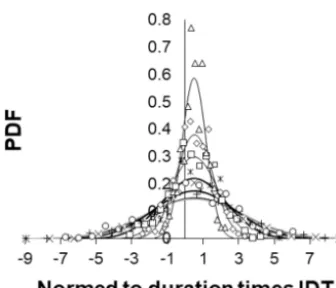
de-Figure 6. PDF of, normed to window length, IDT values calcu-lated for consecutive 100 data windows of simucalcu-lated noise data se-quences, shifted by 100 data. From top to bottom, black curves cor-respond toβ=0.001 (triangles),β=0.275 (diamonds),β=0.545 (squares), β=0.810 (asterisks), β=1.120 (circles), β=1.387 (plus signs), and the grey curve corresponds to β=1.655 (cross signs).

tect differences in considered data sets (in this case norming to the number of data in the window is not necessary because all windows contain the same number of data).

Thus, based on the analysis of specially simulated data se-quences we conclude that the IDT calculation method is ef-fective in detecting small changes occurring in, even short, complex data sets with different dynamical structures. 3.2 Analysis of earthquake time distributions in the

southern California catalog

In this section we proceeded to the analysis of original data sets drawn from the southern California seismic catalog us-ing the IDT calculation approach.

As it was proposed above, for random sequences com-pared to more regular data sets, the sum of the deviation times should approach zero faster in the infinite length limit. Re-sults presented in the previous section confirms this in the example of model random (or random-like) data sets with different extent of regularity (or randomness).

In the case of a real earthquake generation process, which according to present views can not be regarded as completely random (Goltz, 1998; Matcharashvili et al., 2000, 2016; Abe and Suzuki, 2004; Iliopoulos et al., 2012), we should as-sume that the IDTs for the periods with the more random-like earthquake time distributions will be closer to zero, com-pared to the less random ones.

To show this, we used the seismic catalog of southern Cal-ifornia, the most trustworthy database for analysis targeted in this research. Aiming at the analysis of temporal features of seismic process, we intentionally avoided any cleaning or filtering of the catalog in order to preserve its original tempo-ral structure. Therefore, according to common practice (see e.g., Christensen et al., 2002; Corral, 2004) we regard the

seismic processes in this catalog as a whole, irrespective of the details of tectonic features, earthquake location, or their classification as mainshocks or aftershocks.

It was quite understandable that, for such a catalog, we logically should expect time clustering of interdependent events: foreshocks and aftershocks. This, in the context of our analysis, apparently could lead to a considerable amount of events occurring prior to corresponding regular markers (probably mostly aftershocks). Thus, it was interesting to know how the number of events occurred prior to or after regular markers and especially how the result of IDT calcu-lations (which directly depends on the number of events that occurred prior to and after regular markers) is related with the time locations of such interdependent events.

Here we underline the fact that both IDT values as well as the portion of events that occurred prior to or after regular markers (as defined in the methods section) would strongly depend on the position and length of a certain time win-dow in the catalog. Thus, we focused on the whole dura-tion period of the considered catalog (at the representative thresholdM=2.6). We found that in this catalog, 55 % of all earthquakes occurred prior to and 45 % after the regu-lar time markers. To elucidate the role of dependent events on this ratio we analyzed the catalog for higher representa-tive thresholds. At increasedM=3.6 representative magni-tude threshold, we found that the portion of earthquakes oc-curred prior to marker decrease (33 % of all earthquakes). This provided an argument in favor of the assumption that the prevalence of earthquakes, which occur prior to mark-ers, may indeed be related with dependent low-magnitude events (supposedly mostly aftershocks). At the same time, further increase in representative threshold convinces us that dependent low-magnitude events in the catalog may not be the sole cause influencing the amount of earthquakes that oc-curred prior to markers. Indeed, the portion of events that occurred prior to markers increased to 42 % at the representa-tive thresholdM=4.6. Most noticeable is that at the highest considered representative threshold,M=5.6, we observe a further increase in the portion of earthquakes occurring prior to regular markers; to the level observed forM=2.6 thresh-old (55 % of all events). Thus, it seems unlikely that the ratio between events that occurred prior to or after regular markers may be related only with dependent events (aftershocks).

(7)

of earthquakes and to the time span of the catalog. Normed in this way, IDT vales are 0.021, 0.023, 0.022, and−0.030 at representative thresholds M=2.6, M=3.6, M=4.6, and M=5.6 accordingly. It was expected that the increase in the magnitude threshold will make the time distribution of re-mained stronger EQs more random. Indeed, calculated val-ues of IDTs decreased when the representative threshold in-creased. At the same time, normalization to the time span and number of events shows that the time distribution features of stronger earthquakes, in principle, do not differ from smaller ones.

In this sense, it is logical that decreased probability of de-pendent events, at increased representative threshold, do not necessarily cause a proportional increase in the number of occurred after regular markers events, though absolute val-ues of IDT drastically decrease. These results also indicate that the ratio between events, occurred prior to or after regu-lar markers, found for the entire span of SC catalog, as well as the IDT value, should not be reduced only to the distribu-tional features of dependent events.

Further, we needed to clear up whether the ratio of events occurred prior to or after regular markers and especially ob-tained IDT values, are characteristics of the time distributions of earthquakes in the SC catalog or they reflect an influence of some unknown random effects, which are not directly re-lated with the seismic process. For this, we started to calcu-late IDT values for the set of randomized catalogs. In these artificial catalogs, the original time structure of the south-ern California earthquake distributions was destroyed prior to analysis. Specifically, occurrence times of original events have been randomly shuffled (i.e., earthquake time locations have been randomly changed over the entire time span of more than 42 years). We have generated 150 such random-ized catalogs and for each of them IDT values have been cal-culated for the whole catalog time span (which was the same as for the original catalog).

It was found that for the whole period of observation, earthquakes prevailed in 58 % of all time-randomized cata-logs, and occurred prior to the corresponding regular mark-ers. At the same time, unlike the original catalog where 55 % of earthquakes occurred prior to corresponding regular mark-ers, in the randomized catalogs the portion of such earth-quakes, occurred prior to markers, varied in a wide range (from 51 to 92 %). Thus, in spite of some similarity to the portion of events occurred prior to and after regular markers, original and time-randomized catalogs are still different.

Next, comparing the averaged IDT value of random-ized catalogs (calculated from IDTs of 150 randomly shuf-fled catalogs) we found that it is also with minus sign (−159 755 608 min). This was expected since in 58 % of cases of randomized catalogs, prevailed earthquakes oc-curred prior to regular markers. Thus, comparing the average of IDT, calculated for the entire length of randomized cata-logs, with the IDT value of the original SC catalog, we see that the last one is 2 orders of magnitude larger. The

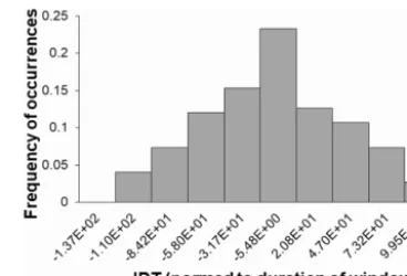
differ-Figure 7.Frequency of occurrences of, normed to the span of win-dow, integral deviation time values (IDTs), calculated for each of the 150 randomized catalogs for the whole period.

ence between IDT of the whole original catalog and the aver-age IDT of randomized catalogs was statistically significant, withZscore=11.2, corresponding top=0.001 (Bevington and Robinson, 2002; Sales-Pardo et al., 2007). For clarity, we add here that IDT values from each of the randomized catalogs was essentially smaller than IDT from the original catalog and thus effects of averaging cannot play any role.

The difference between IDT values calculated for original and time-randomized catalogs is further highlighted in Fig. 7, where normed to the windows span IDT values are presented. We see that in all cases normed-to-windows-span IDTs are clearly smaller than for the original catalog (6.59×102). It is interesting that in at least 30 % of cases, IDTs calculated for randomized catalogs are more than 2 orders smaller than IDT for the original catalog.

From this analysis two important conclusions can be drawn: (i) IDT value, calculated for the considered period of the southern California earthquake catalog, expresses the internal time distribution features of the original seismic pro-cess, and (ii) random-like earthquake time distributions lead to lower (closer to zero) IDT values comparing to the whole original catalog.

All above results obtained for simulated data sets as well as for the time distributions of earthquakes in the original catalog undoubtedly shows that the time distribution of earth-quakes in southern California for the entire period should be regarded as a strongly nonrandom process (IDT is larger than for randomly distributed in time earthquakes). Therefore, the result of this simple statistical analysis is in complete agree-ment with our earlier results, obtained by contemporary non-linear data analysis methods, as well as with the results of similar analysis reported by other authors, which used dif-ferent methodological approaches, see e.g., Goltz (1998), Matcharashvili et al. (2000, 2016), Abe and Suzuki (2004), Telesca et al. (2012), and Iliopoulos et al. (2012).

(8)

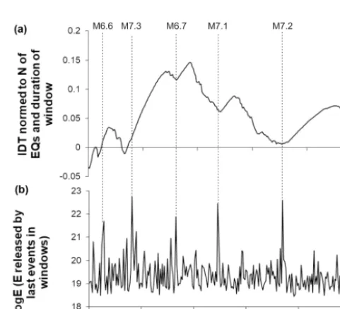
Figure 8.Calculated for extending by 10 consecutive data windows in the southern California earthquake catalog,(a)portion of earthquakes occurred prior to (grey) and after (black) regular markers in each window,(b)normed to the number of EQs and time duration of expanding windows IDTs (top), cumulative amount of released in window seismic energies (bottom).

number of earthquakes that occurred prior to or after corre-sponding regular markers may change depending on the time span of the analyzed catalog. The same can be said about the values of the IDTs. In order to investigate the character of the time variation in IDT values of the SC catalog in differ-ent periods, we fulfilled calculation for the expanding time windows. Specifically, we have calculated IDT values start-ing from the first 100 data (earthquakes), expandstart-ing initial window by the consecutive 10 data to the end of the catalog. In Fig. 8, we see that the number and the time location of earthquakes (relative to regular markers), undergoes essential change, when the length of the analyzed part of the catalog (analyzed window’s length) gradually expands to the end of the catalog (in our case from 1 January 1975 to 23 February 2017).

As it is shown in Fig. 8a, in most of the analyzed windows the majority of earthquakes occurred after regular markers, although there are windows with the opposite behavior. So far, most earthquakes in the windows occurred after regu-lar markers, thus it is not surprising that IDTs calculated for consecutive windows are mostly positive. This is clear from Fig. 8b (upper curve), where we see windows with negative IDTs too. Thus, the values of IDTs calculated for extended windows in different periods vary in a wide range, increasing or decreasing and sometimes coming close to zero.

Here we point out again that based on results of the above analysis, accomplished for simulated data sets and random-ized catalogs, we suppose that when IDT values approache zero, the dynamical features of the originally nonrandom seismic process undergoes qualitative changes and becomes random-like or at least is closer to randomness. In other cases, when IDT values change over time but are far from zero, we observe quantitative changes in the extent of regu-larity of nonrandom earthquake time distributions.

From this point of view it is interesting that earthquake time distributions look more random-like for the relatively quiet periods, when the amount of seismic energy calculated

according to Kanamori (1997) decreased comparing to val-ues released in the neighboring windows prior to or after the strongest earthquakes. This is noticeable in the lower curve of Fig. 8b, where we present cumulative values of seismic energy, calculated for consecutive windows, expanding by 10 events to the end of the catalog. We see that in south-ern California from 1975 to 2017, the strongest earthquakes never occurred in periods when the IDT curve comes close to zero or crosses the abscissa line. To avoid misunderstanding because of restricted visibility in Fig. 8b, we point out here that anM=6.4 earthquake has occurred in the window 256, from the start of the catalog, and the IDT curve crossed the abscissa later in the window 266, from the start of the cata-log. Specifically, this was the nearest expanding window with the IDT value closest to zero, started 100 events later. In real time, crossing of the IDT took place in windows ending 2.5– 3 h after theM=6.4 mainshock.

Results in Fig. 8 also provide interesting knowledge about the relation between IDT and the amount of released seis-mic energy. As we see, the three strongest earthquakes in the southern California earthquake catalog (1975–2017) oc-curred on the rising branch of the IDT curve close or imme-diately after local minima. This local decrease in IDT values, possibly, points to the decreased extent of regularity (or in-creased randomness) in the earthquake temporal distribution in periods prior to the strongest earthquakes in California.

(9)

interaction between events) are significantly different (Lom-bardi and Marzocchi, 2007).

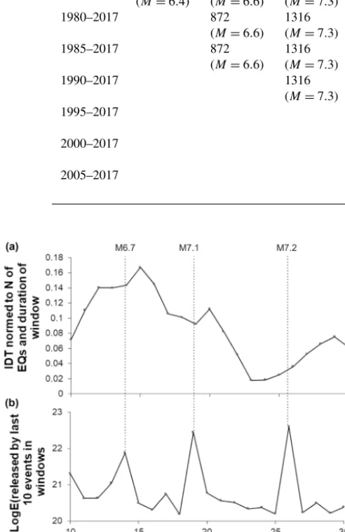
To see how the results of the IDT analysis may be influ-enced by considering smaller or stronger earthquakes, we carried out analysis of the southern California catalog for earthquakes aboveM=3.6 andM=4.6 thresholds. Analy-sis has been accomplished (see results in Figs. 10 and 11) in a manner, similar to the scheme for thresholdM=2.6, i.e., for the entire available period 1975–2017 (e.g., in Fig. 9).

For better visibility of changes in the process of energy re-lease in Figs. 10 and 11 (also in Fig. 9, bottom), we show increments of seismic energy release only calculated for the last 10 events in each consecutive window, opposite to Fig. 8 where we presented energies released by all earthquakes in each window. This was done to make the fine structure of changes in energy release in the expanding (by consecutive 10 events) part of windows more visible, which otherwise is hidden by the strong background level of the summary energy release in the whole window. At the same time, we should not forget that IDTs in Figs. 9–11 are calculated for the entire length of windows and that real evolution of energy release looks similar to that presented in Fig. 8b.

As we see from Figs. 10–11, at higher representative thresholds (similar to lower thresholdM=2.6, in Fig. 9) the strongest earthquakes occur on rising branches of the IDT curve, and that in most cases strong events do no occur in windows where calculated values of IDT come closer to zero. Further analysis by the same scheme for higher-threshold magnitudes (e.g., M=5.6) was impossible because of the scarce number of large earthquakes in the considered seis-mic catalog (just 29 earthquakes above M=5.6). At the same time, we point out that even for M=5.6 representa-tive threshold, for the entire period 1975–2017, the results obtained for two or three available windows (29 events at windows expanding by 9 or 10 data) agree with the above results.

Thus, again we conclude that the increase in magnitude threshold (Figs. 10 and 11) practically do not change the results found for the lower representative threshold. This means that by increasing the representative threshold we still deal with the catalog in which relatively small- and medium-size events prevail. Therefore, conclusions drawn from the analysis for original representative threshold (M=2.6) re-main correct for the case, when we consider a catalog with relatively stronger events; thus, it seems that there is no prin-cipal difference in the character of the contribution of smaller and stronger events to the results of the IDT calculation. Comparison with the results obtained for time-randomized catalogs confirms this conclusion.

Next, in order to avoid doubts related to the fixed start-ing point in the above analysis, we have carried out the same calculation of IDT values for catalogs which started in 1985, 1990, 1995, 2000, and 2005. As it follows from Tables 1 to 3, analysis carried out on shorter catalogs confirm the result ob-tained for the entire period of observation (1975–2017) and

Figure 9.Calculated for the expanding (by consecutive 10 data) windows, integral deviation times (IDTs)(a)and the increments of seismic energies released by 10 last events in consecutive win-dows(b)obtained from the southern California earthquake catalog (above thresholdM=2.6). By the grey lines we show where the IDT curve crosses the abscissa. Dashed lines show the occurrence of largest earthquakes in the catalog.

(10)

Table 1.Comparison between expanding by 10 data windows with the strongest earthquakes occurrences and windows with IDT values closest to zero. Representative thresholdM=2.6.

Catalog Sequential number of expanding windows time span

1975–2017 256 (M=6.4)

921 (M=6.6)

1365 (M=7.3)

1822 (M=6.7)

2194 (M=7.1)

2813 (M=7.2)

2620 (closest to zero value)

1980–2017 872

(M=6.6) 1316 (M=7.3)

1773 (M=6.7)

2145 (M=7.1)

2764 (M=7.2)

1985–2017 872

(M=6.6) 1316 (M=7.3)

1773 (M=6.7)

2145 (M=7.1)

2764 (M=7.2)

1990–2017 1316

(M=7.3) 1773 (M=6.7)

2145 (M=7.1)

2764 (M=7.2)

1995–2017 2145

(M=7.1) 2764 (M=7.2)

2000–2017 2764

(M=7.2)

2005–2017 2764

(M=7.2)

Figure 11.Calculated for the expanding (by consecutive 10 data) windows, integral deviation times (IDTs) (a)and the increments of seismic energies released by 10 last events in consecutive win-dows(b)obtained from the southern California earthquake catalog (above threshold M=4.6). Dashed lines show the occurrence of the largest earthquakes in the catalog.

convinces us that the calculated values of IDT practically never come closer to zero in windows when the strongest earthquakes occur. The only exception is the case ofM=6.6 earthquake at representative thresholdM=3.6 for the period 1975–2017.

Thus, we see that shortening the time span of the analyzed part of the catalog does not influence the obtained results.

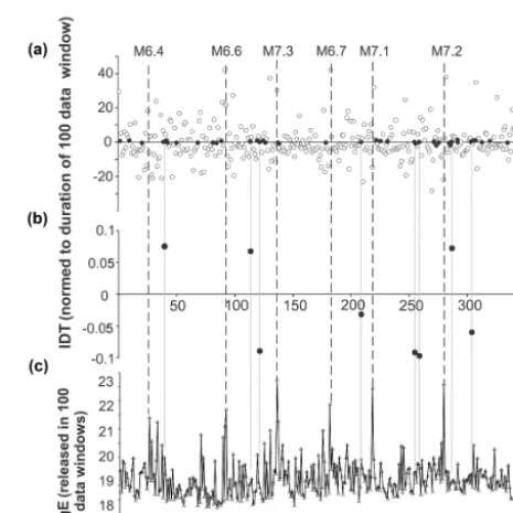
Because of the above-mentioned unclearness in Figs. 9– 11, when we calculated IDTs for the expanding windows and discuss results for the energy release occurred in the last 10 data windows, we performed additional analysis on the sliding windows with fixed number of events. In detail, in the southern California earthquake catalog we have calcu-lated IDT values for non-overlapping windows of 100 con-secutive events, shifted by 100 data (Figs. 12, 13). We have used short-sliding windows of 100 data for two reasons: (i) to have good resolution of changes occurring in the time distri-bution of earthquakes and (ii) because even relatively short, 100 data span windows also provide good enough discrimi-nation in the IDT values, as it is shown in Figs. 5b and 6.

(11)

Table 2.Comparison between expanding by 10 data windows with the strongest earthquakes occurrences and windows with IDT values closest to zero. Representative thresholdM=3.6.

Catalog Sequential number of expanding windows time span

1975–2017 64 (M=6.6)

91 (M=7.3)

133 (M=6.7)

173 (M=7.1)

235 (M=7.2)

64 (closest to zero value) 1980–2017 64

(M=6.6) 91 (M=7.3)

133 (M= 6.7)

173 (M=7.1)

235 (M=7.2)

(M=6.6) 91 (M=7.3)

133 (M=6.7)

173 (M=7.1)

235 (M=7.2)

1990–2017 91

(M=7.3) 133 (M=6.7)

173 (M=7.1)

235 (M=7.2)

1995–2017 173

(M=7.1) 235 (M=7.2)

2000–2017 235

(M=7.2)

2005–2017 235

(M=7.2)

Table 3.Comparison between expanding by 10 data windows with the strongest earthquakes occurrences and windows with IDT val-ues closest to zero. Representative thresholdM=4.6.

catalog Sequential number of expanding windows time span

1975–2017 14 (M=6.7)

19 (M=7.1)

26 (M=7.2)

(M=6.7) 19 (M=7.1)

26 (M=7.2)

(M=6.7) 19 (M=7.1)

26 (M=7.2)

(M=6.7) 19 (M=7.1)

26 (M=7.2)

1995–2017 19

(M=7.1) 26 (M=7.2)

2000–2017 26

(M=7.2)

Results obtained for non-overlapping sliding windows of fixed length also confirm the results obtained for expanding windows.

The simple statistical approach used here thus shows that the extent of randomness in the earthquake time distributions is changing over time and that it is most random-like at pe-riods of decreased seismic activity. The results of this analy-sis provide additional indirect arguments in favor of our ear-lier suggestion that the extent of regularity in the earthquake time distributions should decrease in seismically quiet peri-ods and increase in periperi-ods of strong earthquakes preparation (Matcharashvili et al., 2011, 2013).

(12)

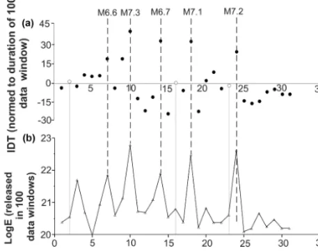
Figure 13. Calculated for the non-overlapping 100 data windows (shifted by 100 data), integral deviation times (IDTs) (circles in panela) and the released seismic energies (triangle in panelb). IDT values in vicinity of 0.1σ from zero are given by open circles in panel(a). By grey lines we show location of closest to zero IDT values relative to the released seismic energy. Dashed lines show the occurrence of largest earthquakes in the southern California cat-alog (above thresholdM=3.6).

4 Conclusions

We investigated earthquake time distributions in the south-ern California earthquake catalog by the method of calcu-lation of integral deviation times (IDTs) relative to regular time markers. The main goal of the research was to quan-tify when the time distribution of earthquakes become closer to the random process. Together with IDT calculation, stan-dard methods of complex data analysis such as power spec-trum regression, Lempel and Ziv complexity, and recurrence quantification analysis, as well as multiscale entropy calcu-lations, have been used. Analysis was accomplished for dif-ferent time intervals and for difdif-ferent magnitude thresholds. Based on a simple statistical analysis result, we infer that the strongest earthquakes in southern California occur only in windows with rising values of IDTs and that the character of the temporal distributions of earthquakes in these windows is less random-like compared to the periods of decreased local seismic activity.

Data availability. The used catalogue is available from http://www. isc.ac.uk/iscbulletin/search/catalogue/ (International Seismological Centre, 2018).

Author contributions. Authors contributed in accordance to their competence in the research subject. Main author TM was respon-sible for all aspects of research and manuscript preparation, TH and TC contributed through commenting and discussion of results, NZ

contributed through the programming, data analysis, and also ac-tively participated in manuscript preparation.

Competing interests. The authors declare that they have no conflict of interest.

Acknowledgements. This work was supported by Shota Rustaveli National Science Foundation (SRNSF), grant 217838 “Inves-tigation of dynamics of earthquake’s temporal distribution”. Takahiro Hatano gratefully acknowledges the support from the MEXT under “Exploratory Challenge on Post-K computer” (Frontiers of Basic Science: Challenging the Limits), the JSPS KAKENHI Grant JP16H06478, and the Earthquake Research Institute cooperative research program.

Edited by: Norbert Marwan

Reviewed by: two anonymous referees

References

Abe, S. and Suzuki, N.: Scale-free network of earthquakes, Euro-phys. Lett., 65, 581–586, 2004.

Aboy, M., Hornero, R., Abásolo, D., and Álvarez, D.: Interpretation of the lempel-ziv complexity measure in the context of biomed-ical signal analysis, IEEE T. Bio-Med. Eng., 53, 2282–2288, 2006.

Beran, J., Feng, Y., Ghosh, S., and Kulik, R.: Long-Memory Processes: Probabilistic Properties and Statistical Methods, Springer, Berlin, Heidelberg, Germany, 2013.

Bevington, P. and Robinson, D. K.: Data Reduction and Error Anal-ysis for the Physical Sciences, 3rd edn., McGraw-Hill, New York, USA, 2002.

Chelidze, T. and Matcharashvili, T.: Complexity of seismic process; measuring and applications, A review, Tectonophysics, 431, 49– 60, 2007.

Chou, C. M.: Applying Multiscale Entropy to the Complexity Anal-ysis of Rainfall-Runoff Relationships, Entropy, 14, 945–957, https://doi.org/10.3390/e14050945, 2012.

Christensen, K., Danon, L., Scanlon, T., and Bak, P.: Unified scaling law for earthquakes, P. Natl. Acad. Sci. USA, 99, 2509–2513, 2002.

Corral, A.: Long-term clustering, scaling, and universality in the temporal occurrence of earthquakes, Phys. Rev. Lett., 92, 108501, https://doi.org/10.1103/PhysRevLett.92.108501, 2004. Costa, M., Goldberger, A. L., and Peng, C. K.: Multiscale

en-tropy analysis of biological signals, Phys. Rev. E, 71, 021906, https://doi.org/10.1103/PhysRevE.71.021906, 2005.

Cover, T. M. and Thomas, J. A.: Elements of Information Theory, Wiley, New York, USA, 1991.

Davidsen, J. and Goltz, C.: Are seismic waiting time dis-tributions universal?, Geophys. Res. Lett. 31, L21612, https://doi.org/10.1029/2004GL020892, 2004.

Eckmann, J. P., Kamphorst, S., and Ruelle, D.: Recurrence plots of dynamical systems, Europhys. Lett., 4, 973–977, 1987. Goltz, C.: Fractal and Chaotic Properties of Earthquakes, in:

(13)

Hu, J., Gao, J., and Principe, J. C.: Analysis of Biomedi-cal Signals by the Lempel-Ziv Complexity: the Effect of Finite Data Size, IEEE T. Bio-Med. Eng., 53, 2606–2609, https://doi.org/10.1109/TBME.2006.883825, 2006.

Iliopoulos, A. C., Pavlos, G. P., Papadimitriou, P. P., Sfiris, D. S., Athanasiou, M. A., and Tsoutsouras, V. G.: Chaos, selforganized criticality, intermittent turbulence and nonextensivity revealed from seismogenesis in north Aegean area, Int. J. Bifurcat. Chaos, 22, 1250224, https://doi.org/10.1142/S0218127412502240, 2012.

International Seismological Centre: Southern California earth-quake catalog, Berkshire, UK, available at: http://www.isc.ac.uk/ iscbulletin/search/catalogue/, last access: 5 July 2018.

Kanamori, H.: The energy release in great earthquakes, J. Geophys. Res., 82, 2981–2987, 1977.

Kasdin, N. J.: Discrete simulation of colored noise and stochastic processes and 1/f power law noise generation, Proceedings of the IEEE, 83,802–827, 1995.

Lempel, A. and Ziv, J.: On the complexity of finite sequences, IEEE T. Inform. Theory, IT-22, 75–81, 1976.

Lennartz, S., Livina, V. N., Bunde, A., and Havlin, S.: Long-term memory in earthquakes and the distribution of interoccurrence times, Europhys. Lett., 81, 69001, https://doi.org/10.1209/0295-5075/81/69001, 2008.

Lombardi, A. M. and Marzocchi, W.: Evidence of cluster-ing and nonstationarity in the time distribution of large worldwide earthquakes, J. Geophys. Res., 112, B02303, https://doi.org/10.1029/2006JB004568, 2007.

Malamud, B. D. and Turcotte, D. L.: Self-affine time series I: Gen-eration and analyses, Adv. Geophys., 40, 1–90, 1999.

Martínez, M. D., Lana, X., Posadas, A. M., and Pujades, L.: Statisti-cal distribution of elapsed times and distances of seismic events: the case of the Southern Spain seismic catalogue, Nonlin. Pro-cesses Geophys., 12, 235–244, https://doi.org/10.5194/npg-12-235-2005, 2005.

Marwan, N., Romano, M. C., Thiel, M., and Kurths, J.: Recurrence plots for the analysis of complex system, Phys. Rep. 438, 237– 329, 2007.

Matcharashvili, T., Chelidze, T., and Javakhishvili, Z.: Nonlinear analysis of magnitude and interevent time interval sequences for earthquakes of the Caucasian region, Nonlin. Processes Geo-phys., 7, 9–20, https://doi.org/10.5194/npg-7-9-2000, 2000. Matcharashvili, T., Chelidze, T., Javakhishvili Z., and Ghlonti, E.:

Detecting differences in dynamics of small earthquakes temporal distribution before and after large events, Comput. Geosci., 28, 693–700, 2002.

Matcharashvili, T., Chelidze, T., Javakhishvili, Z., Jorjiashvili, N., and FraPaleo, U.: Non-extensive statistical analysis of seismicity in the area of Javakheti, Georgia, Comput. Geosci., 37, 1627– 1632, 2011.

Matcharashvili, T., Telesca, L., Chelidze, T., Javakhishvili, Z., and Zhukova, N.: Analysis of temporal variation of earthquake oc-currences in Caucasus from 1960 to 2011, Tectonophysics, 608, 857–865, 2013.

Matcharashvili, T., Chelidze, T., Javakhishvili, Z., and Zhukova, N.: Variation of the scaling characteristics of temporal and spatial distribution of earthquakes in Caucasus, Physica A, 449, 136– 144, 2016.

Milotti, E.: New version of PLNoise: a package for exact numerical simulation of power-law noises, Comput. Phys. Commun., 177, 391–398, 2007.

Munoz-Diosdado, A., Guzman-Vargas, L., Rairez-Rojas, A., Del Rio-Correa, J. L., and Angulo-Brown, F.: Some cases of crossover behavior in heart interbeat and electoseismic time se-ries, Fractals, 13, 253–263, 2005.

Peng, C. K., Buldyrev, S. V., Havlin, S., Simons, M., Stanley, H. E., and Goldberger, A. L.: Mosaic organization of DNA nucleotides, Phys. Rev. E, 49, 1685–1689, 1994.

Peng, C. K., Havlin, S., Stanley, H. E., and Goldberger, A. L: Quantification of scaling exponents and crossover phenom-ena in nonstationary heartbeat time series, Chaos, 5, 82–87, https://doi.org/10.1063/1.166141, 1995.

Richman, J. S. and Moorman, J. R.: Physiological time-series anal-ysis using approximate entropy and sample entropy, Am. J. Physiol.-Heart C., 278, H2039–H2049, 2000.

Rukhin, A., Soto, J., Nechvatal, J., Smid, M., Barker, E., Leigh, S., Levenson, M., Vangel, M., Banks, D., Heckert, A., Dray, J., and Vo, S.: The Statistical Tests Suite for Random and Pseudo-random Number Generators for Cryptographic application, NIST Special Publication 800-22revla, National Institute of Standards and Technology, Gaithersburg, USA, 2010.

Sales-Pardo, M., Guimer, R., Moreira, A. A., and NunesAmaral, L. A.: Extracting the hierarchical organization of complex systems, P. Natl. Acad. Sci. USA, 104, 14224–15229, 2007.

Schaefer, A., Brach, J. S., Perera, S., and Sejdic, E.: A compara-tive analysis of spectral exponent estimation techniques for 1/f processes with applications to the analysis of stride interval time series, J. Neurosci. Meth., 222, 118–130, 2014.

Shlesinger, M. F.: Fractal time and 1/f noise in complex systems, Ann. NY Acad. Sci., 504, 214–228, 1987.

Stadnitski, T.: Measuring fractality, Front. Physio, 3, 1–10, https://doi.org/10.3389/fphys.2012.00127, 2012.

Telesca, L., Cuomo, V., Lapenna, V., and Macchiato, M.: Identify-ing space–time clus-terIdentify-ing properties of the 1983–1997 Irpinia-Basilicata (Southern Italy) seismicity, Tectonophysics, 330, 93– 102, 2001.

Telesca, L., Matcharashvili, T., and Chelidze, T.: Investigation of the temporal fluctuations of the 1960–2010 seismicity of Caucasus, Nat. Hazards Earth Syst. Sci., 12, 1905–1909, https://doi.org/10.5194/nhess-12-1905-2012, 2012.

Webber, C. L. and Marwan, N. (Eds.): Recurrence Quantification Analysis Theory and Best Practices, Springer International Pub-lishing, Cham, Switzerland, https://doi.org/10.1007/978-3-319-07155-8, 2015.

Webber, C. L. and Zbilut, J.: Dynamical assessment of physiolog-ical systems and states using recurrence plot strategies, J. Appl. Physiol., 76, 965–973, 1994.

Webber, C. L. and Zbilut, J. P.: Recurrence quantification analysis of nonlinear dynamical systems, in: Tutorials in contemporary non-linear methods for the behavioral sciences, edited by: Riley M. A. and Van Orden G. C., National Science Foundation Program in Perception, Action and Cognition, 26–94, available at: https: //www.nsf.gov/pubs/2005/nsf05057/nmbs/nmbs.pdf (last access: 5 July 2018), 2005.

(14)

Anal-ysis as a general purpose data analAnal-ysis tool, Phys. Lett. A, 373, 3753–3756, 2009.

Wu, S. D., Wu, C. W., Lin, S. G., Wang, C. C., and Lee, K. Y.: Time Series Analysis Using Composite Multiscale Entropy, Entropy, 15, 1069–1084, 2013a.

Wu, S. D., Wu, C. W., Lee, K. Y., and Lin, S. G.: Modified multi-scale entropy for short-term time series analysis, Physica A, 392, 5865–5873, 2013b.