DEVELOPMENT OF DELAY MODELS USING SIMULATION IN A
HETEROGENEOUS TRAFFIC CONDITION
Sheela Alex1 , Kuncheria P. Isaac2
1Government Engineering College, Thrissur, India. 2Kerala Technological University, Trivandrum, India
Received 26 June 2016; accepted 29 August 2016
Abstract: The behaviour of traffic system in a heterogeneous traffic condition is entirely different from that of a homogeneous condition. The awareness of the influence of heterogeneity in a road network is essential for the planners and designers of the transportation system. Vehicle delay is perhaps the most important parameter used by transportation professionals to measure the performance of signalised intersections. In a mixed traffic condition, the vehicle delays are influenced by many traffic stream characteristics, taking into consideration of vehicular as well as traffic characteristics. The paper highlights the need for developing the delay models under various vehicular interactions for mixed traffic conditions prevalent in India. Experiments were carried out using the micro simulation model, TRAFFICSIM, which was developed for signalised intersections by the authors and reported elsewhere. As an application of the model TRAFFICSIM, the effect of traffic composition on delay is estimated. Considering both the delay and the flow ratio, the concept of Level of Service at signalised intersection in a mixed traffic condition, is mentioned in the paper. Influence of the proportion of buses and three wheelers in the determination of LOS are also presented.
Keywords: dynamic PCU, simulation, TRAFFICSIM, mixed traffic, delay, flow ratio, Level of Service.
1. Introduction
Due to the random variations in traffic flow in a mixed traffic condition, it is very difficult to accurately predict the vehicle delays at signalised intersections. The delay that a particular vehicle experiences when it travels through an approach to a signalised intersection depends on a number of factors including the probabilistic distribution of arrival flow, signal timings, and the varying operating characteristics of different vehicle types.
Delay was computed based on the concept that the difference in travel time experienced
by the vehicle when it is moving in a signal and when it is having a continuous movement along a certain stretch of the road. This delay is considered as the total control delay due to intersection and it includes stopped delay, acceleration and deceleration delay. For this, the authors have developed a microscopic traffic simulation model, TRAFFICSIM, which was reported elsewhere. The analysis was limited to the development of delay models for straight movements only and no turning movements were considered.
signal timings. If no queue is present when a vehicle arrives during green interval, it can be immediately discharged without delay. Otherwise the vehicle waits until the queued vehicles ahead of it discharged completely. The vehicle which arrives during the red time experiences the overall delay as it accumulates and forming a queue which includes the initial deceleration delay, stopped delay as well as the acceleration delay when the vehicle starts discharging as the signal turns green.
2. Literature Review
Delay at intersections is one of the key parameters that are utilised in the optimisation of traffic signal timings. It plays an important role in computing the Level Of Service provided to traffic at signalised intersections. Typically two types of analysis can be done, a deterministic analysis and a stochastic analysis. In a deterministic analysis, the vehicle arrivals are assumed to follow a uniform pattern whereas in a stochastic analysis, it is assumed to follow some probability distributions. Using deterministic queuing analysis, (Webster and Cobbe, 1966) developed a model for estimating the delay incurred by motorists at under saturated signalised intersections that became the basis for all subsequent delay models.
(Olszewski, 1993) reported that for the overflow stopped delay component, the delay ratio depends on cycle time and the degree of saturation. (Benekohal and Zohairy, 1993) presented a new set of progression adjustment factors (PF) using the arrival based delay models. (Arasan and Jagadeesh, 1995) adopted a probabilistic approach based on first order second moment method to estimate the saturation f low and delay
caused to traffic at signalised intersections under heterogeneous traffic conditions and was found close to the observed values of delay. (Fu and Hellinga, 2000) developed an analytical model to estimate the variance of overall delay, including the variance of uniform delays and the variation of random delays. The variance of delays was directly calibrated from the simulation data. Hence it might not take the actual demand variations into considerations.
(Dion et al., 2004) compared the delays that were estimated by a number of existing analytical models for a signalised intersection approach controlled in fixed time and operated in a range extending from under saturated to highly saturated and the results indicated that all delay models produce similar results for signalised intersections with low traffic demand, but increasing differences occur as the traffic demand approaches saturation.
(Sazi Murat and Baskan, 2006) adopted an Artificial Neural Network (ANN) approach for modelling vehicle delays at signalised junctions. (Hoque and Imran, 2007) developed a modified Webster’s delay model, to suit the road traffic situations of Bangladesh. (Akgungor, 2008) proposed a methodology and a new formulation to identify the delay parameters in the delay model. A new method of Incremental Queue Accumulation (IQA) for calculating uniform delay was proposed by (Strong and Rouphail, 2006), for inclusion in HCM 2010. (Minh et al., 2009) proposed a modified Webster’s model to estimate delay for heterogeneous traffic conditions at pre-timed signalised intersections.
signalised intersections in China. The results showed that the delays mainly depend on the proportion and positions of heavy vehicles in the queue, as well as the start up situations (with or without interference). (Mulandi and Martin, 2011) developed models to modify the IQA method to provide more accurate estimates of left turns and was validated for different configurations such as protected plus permitted lefts from an exclusive lane, permitted lefts from an exclusive lane and shared lanes with permitted lefts. In the (HCM, 2010), the average delay per vehicle for a lane group is given as the sum of the uniform delay, the incremental or random delay and the residual demand delay to account for the over saturation queues.
(Bhuyan and Rao, 2011) carried out studies on delay at signalised intersections in the city of Mumbai and the result was validated for KolKata city. They considered K means clustering as the most suitable method in defining LOS categories. The results showed that the intersection delay ranges for LOS categories valid in Indian context were much higher and were approximately two times to those values mentioned in (HCM, 2010). (Al-Kubaisi, 2012) conducted a study on the vehicle behaviour and delay at signalised intersections at Baghdad city and developed a regression model for predicting the optimum cycle time, based on simulation model developed from observed driver behaviour.
(Kumar and Dhinakaran, 2012) discussed the various problems associated with delay estimation under mixed traffic conditions in a developing country and an attempt was made to improve the accuracy of the delay estimation. Even after taking several measures, the study could not obtain a good correlation between observed and predicted
suggested by (Bhuyan and Rao, 2011) to assign LOS grades of study intersections. The study also suggested that selection of an appropriate method of PCU estimation can significantly improve the accuracy of delay calculations.
(Das et al., 2013) conducted a study for defining LOS categories for highly heterogeneous traffic condition for urban streets using Neural Gas clustering technique and confirmed that the free flow speed ranges for different urban street classes and speed ranges for different LOS categories were found to be lower than that suggested by (HCM, 2010).
3. Objectives and Scope of the Work
The objective of the research work presented in the paper is to determine the effect of traffic composition on delay at signalised intersections. (Sheela and Isaac, 2014) recently developed a traffic simulation model, TR AFFICSIM, which was used to study the vehicular interactions, at micro level over a wide range of traffic flow conditions at signalised intersections. Moreover, (Sheela and Isaac, 2014) developed traffic simulation model and its application for estimating saturation flow at signalised intersections. Dynamic PCU values at signalised intersections in India for mixed traffic are determined by (Sheela and Isaac, 2015). LOS criteria for a mixed traffic condition were also suggested based on control delay and flow ratio as well as proportion of three wheelers.
4. Methodology
varying the traffic composition with a signal timing consisted of a cycle time of 120 s, with an effective green interval of 56 s, amber period of 4 s and a red time of 60 s. The analysis was done on a carriageway width of 7 m. Control stretch for the extraction of data for delay estimation was selected in such a way that the first control point was 50 m ahead of the stop line and the last point just clears the intersection. Travel time was estimated as the time interval by which the particular vehicle crosses the control points. Simulation model was also run for 15 minutes having a continuous movement of traffic providing green time for the entire cycle time for assessing the travel time without delay.
4.1 Delay in a Single Vehicle Traffic
Stream
Simulation runs were done on a single vehicle traffic stream, consisting either car or bus or two wheeler or three wheeler only. The data was further analysed and the results of this analysis is tabulated in Table 1 where the average delay in each situation was estimated and the percentage variation in delay with respect to car only condition is determined.
The simulation model was run with traffic volume at saturation level i.e. maximum flow possible at the intersection approach, to obtain the delay in Table 1 and 2.
Table 1
Average Delay per Vehicle in a Single Vehicle Only Traffic Stream
Traffic Composition
Average Travel Time per Vehicle (s) Average Delay (s)
Variation of Delay with Respect to Car Only
Condition With Signal Continuous Movement
car only 62.97 4.17 58.80
-two wheeler only 50.20 4.89 45.31 Decreases by 23%
three wheeler only 63.14 5.71 57.43 Decreases by 2.3%
bus only 68.36 6.09 62.27 Increases by 6%
As expected, it was seen that when there is a condition of two wheeler only instead of car only, the delay decreases by 23%. This may be due to the fact that the two wheelers could gain their speed in the absence of heavy vehicle and also that the total passenger car units in the traffic stream would be less. As the acceleration and speed characteristics of three wheelers and cars are almost same within the range of speeds of about 0 to 30 kmph, there is only slight variation of delay in a three wheeler only condition when compared with car only stream. Because of the variation in the physical and operating characteristics of bus, the average delay increases by 6% in a bus only condition when compared to car only stream.
4.2 Delay in a Two Vehicle Traffic Stream
In order to analyse the effect of two wheeler, three wheeler or bus with car, simulation runs were made by varying the percentage composition of t wo wheelers, three wheelers or buses in complementary with the percentage of cars. Five compositions were tried for each combination as given in Table 2. The results were analysed and the difference in delay for the said combinations with the car only stream are tabulated and are shown in Table 2.
with three wheeler, the variation in delay doesn’t show any trend as there is not much variation in the speed characteristics as well as operating characteristics of the two vehicles. However when up to 70% of cars replaced by three wheelers, there shows no variation in delay as the mutual interaction
between them are almost the same. In car and bus combination, variation in delay is occurred when more than 10% cars are replaced by buses. This is because as the percentage of bus increases, there must be the reduction in stream speed which increases the average delay per vehicle in the traffic stream.
Table 2
Average Delay per Vehicle in a Two Vehicle Traffic Stream
Type of Vehicle Combination
Traffic
Composition (%) Travel Time (s) Delay (s) Delay with Respect to Car Only (%) Car Vehicle With Signal Continuous Movement Increases Decreases
car-two wheeler
90 10 63.2 4.47 58.73 negligible
70 30 60.80 4.85 55.95 - 4.80
50 50 57.10 5.45 51.65 - 12.20
30 70 54.80 5.50 49.30 - 16.16
10 90 51.65 5.85 45.80 - 22.10
car-three wheeler
90 10 62.84 4.56 58.28 negligible
70 30 62.83 4.60 58.23 negligible
50 50 63.19 5.11 58.08 negligible
30 70 63.59 5.53 58.06 negligible
10 90 63.41 5.71 57.73 - 1.80
car-bus
90 10 63.11 4.47 58.64 negligible
70 30 66.04 4.85 61.19 4.00
-50 50 67.54 5.45 62.09 5.59
-30 70 67.60 5.50 62.10 5.61
-10 90 68.02 5.85 62.17 5.73
-To study the effect of the lesser flow on the delay, simulation runs were conducted for different combinations for varying traffic volumes from 600 to 4000 veh/hr in suitable steps and average delay values were arrived. The obtained delay values were plotted for the possible combinations and are given in Figs.1, 2 and 3.
From Fig.1 to 3, it is noticed that the variation of delay for varying percentage compositions of car and other vehicle combination shows the same trend as predicted, i.e. when the traffic
c – 2w*
(*c – 2w represents percentage of cars and two wheelers) Fig. 1.
Variation of Delay for Car-Two Wheeler Combination
c – 3w*
(*c – 3w represents percentage of cars and three wheelers) Fig. 2.
Variation of Delay for Car-Three Wheeler Combination
c - b*
(*c - b represents percentage of cars and buses) Fig. 3.
4.3. Delay in a Mixed Traffic Stream
For analysing the effect of all vehicle types on delay, simulation runs were done by varying the proportions of different vehicle types. Three different cases were considered. In the first case, the traffic composition selected
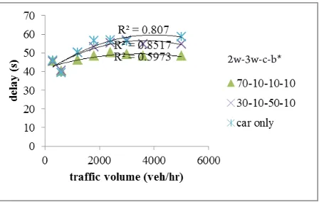
was by varying the percentage compositions of cars and two wheelers, thereby keeping the percentage of three wheeler and bus constant at 10%. Figure 4 shows the variation in delay for varying two wheeler and car in a mixed traffic condition and is shown along with a car only condition.
2w-3w-c-b*
(*2w-3w-c-b represents percentage of two wheelers, three wheelers, cars and buses) Fig. 4.
Delay for Varying Proportion of Two Wheeler in a Mixed Traffic
Figure 4 shows that when the percentage of two wheeler increases and the proportion of car decreases, the delay of vehicles at that approach is less compared to a decrease in two wheeler and increase in car proportion. This may be due to the fact that as the proportion of two wheeler increases with the corresponding decrease in the proportion of car, two wheelers can gain speed and also the flow ratio (flow to saturation flow) reduced, thereby reducing the delay.
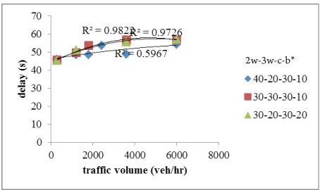
In the second case, the proportion of bus and car varied, keeping the percentage
2w-3w-c-b*
(*2w-3w-c-b represents percentage of two wheelers, three wheelers, cars and buses) Fig. 5.
Delay for Varying Proportion of Bus in a Mixed Traffic
From Fig. 5, it was noticed that as percentage of bus increases, the delay is more, compared to all the other cases. The manoeuvrability of bus is less compared to other modes of transport and hence as
proportion increases, the stream speed decreases and hence more delay occurs. Also as the proportion of bus increases, the corresponding flow ratio increases, this increases the delay.
2w-3w-c-b*
(*2w-3w-c-b represents percentage of two wheelers, three wheelers, cars and buses) Fig. 6.
Delay for all Vehicle Combination for Varying Traffic Volumes
From Fig. 6, it is obser ved that the combination of 40% two wheelers, 20% three wheelers, 30% cars and 10% buses gives a delay of 54 s compared to other combinations having a delay of 57 s at
5. Effect of Varying Proportion of Traffic
on Flow Ratio
The flow ratio depends upon many factors such as carriageway width, saturation flow, proportion of traffic and traffic volume. For studying the effect of flow ratio with varying proportion of traffic, simulation runs were made for varying traffic composition and for varying traffic volume. Analysis was done for different proportion of traffic along a stretch of uniform carriageway width of 7 m and having a constant saturation flow of 3656 PCU/hr as obtained in the study referred by
the authors. Flow ratio was obtained as the ratio of flow in PCU/hr to saturation flow. Flow in PCU/hr was obtained by multiplying the number of vehicles of each category by the corresponding dynamic PCU values based on the composition of traffic. Dynamic PCU value based on the composition was obtained from the developed PCU models referred by the authors (Sheela and Isaac, 2015). Multiple linear regression analysis was done with flow ratio (q/s) as dependant variable and proportion of traffic as independent variables as given in Eq.1 which provides good statistical results.
(1)
where, two_wheeler, three_wheeler, car
and bus, represents the proportions of two wheeler, three wheeler, car and bus respectively. The regression statistics of the model gives a standard error of 0.18 and R2 value of 0.88. The t-values obtained for the variables two_wheeler, three_wheeler, car and bus are 3.165, 5.895,1.826 and 9.024 respectively which are higher than the critical value for all the cases and are having a high coefficient of determination which shows that the model is statistically significant.
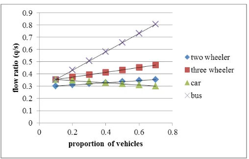
Effect of the proportion of vehicles on flow ratio is shown in Fig. 7. The graph was obtained by varying the proportion of each vehicle type from 10 to 70% in
complementary with any other vehicle, keeping the proportions of any two vehicles at 10%.
Fig. 7.
Flow Ratio for Varying Proportion of Vehicles
6. Development of a Composite Delay
Model
Delay studies so far carried out were for limited variables and mostly done in a homogeneous traffic condition and hence it is necessary to develop a composite model incorporating the composition of all the four vehicle types and the flow ratio. But the flow ratio could not be given as an independent variable, since they are mutually related
with proportions of vehicles. The delay estimated from the analysis of the output values of the simulation model were used to develop a composite delay model. The analysis showed that a linear regression gives the best statistical fit and a linear regression model was developed with average delay per vehicle as dependant variable and proportions of vehicles as independent variables. The developed model is given in Eq. 2:
(2)
where, delay is the average control delay per vehicle, car,two_wheeler, three_wheeler, and
bus indicates the proportions of car, two wheeler, three wheeler and bus respectively. The regression statistics of the model gives a standard error of 5.33 and R2 value of 0.96, which indicate that the model explained a large portion of the variations in the simulated delay data. The t-values obtained
for the variables two_wheeler, three_wheeler, car and bus are 17.531, 13.955,13.809 and 18.605 respectively which are higher than the critical value at the 5% level of significance which indicates that the included parameters are statistically significant.
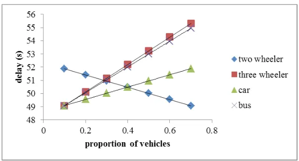
in complementary with another vehicle and the other two proportions kept as constant, variation in delay was analysed and is presented in Fig. 8. From the figure, it can be seen that the results are as expected i.e. as the proportion of vehicles increases in the mix, the delay increases. There is an exception for this in the case of two wheelers. As the proportion of two wheelers increases, the delay decreases. It was also found that when the proportion of two wheeler is less than 0.3, the delay is more corresponding to the same proportion of other vehicles i.e. when the proportion of two wheeler
is 0.2, the average delay per vehicle in the traffic stream is 51.4 s, whereas when the proportion of three wheeler, car and bus in a traffic stream is 0.2 corresponding average delay per vehicle in the traffic stream is 50 s, 49.5 s and 50 s respectively. This is because, when the proportion of two wheeler is less than 0.3, the corresponding proportions of other vehicles are more, which resulted in more delay. As bus and three wheelers are considered as the commonly adopted public modes of transport, this contributes a major role for increasing the delay in an urban environment.
Fig. 8.
Variation in Delay for Varying Proportion Of Vehicles
6.1. Effect of Flow Ratio on Delay
In a mixed traffic condition, flow ratio depends upon the proportion of each category of vehicle type and it has been found that same flow ratio can occur for different
2w-3w-c-b*
(*2w-3w-c-b represents percentage of two wheelers, three wheelers, cars and buses) Fig. 9.
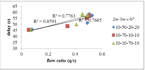
Variation of Delay with Flow Ratio for Varying Bus and Car
2w-3w-c-b*
(*2w-3w-c-b represents percentage of two wheelers, three wheelers, cars and buses) Fig. 10.
Variation of Delay with Flow Ratio for Varying Two Wheeler and Car
2w-3w-c-b*
(*2w-3w-c-b represents percentage of two wheelers, three wheelers, cars and buses) Fig. 11.
From Fig. 9, it was observed that, the flow ratio increases for a particular variation in traffic volume, up to 1.0 with an increase in proportion of bus, whereas flow ratio varies less than 0.5 for the variation in proportion of two wheeler and it varies up to 0.6 for an increase in proportion of three wheeler as seen in Fig.10 and 11. This is due to the variation in dynamic PCU values of each vehicle type for different traffic compositions. It is also inferred that for the same flow ratio, the delay gets varied as it depends upon the proportion of vehicles and the traffic volume and thus it clearly justified the influence of flow ratio and the proportion of vehicle types especially the proportion of bus in the estimation of delay.
7. Determination of Level Of Service
(LOS) in Mixed Traffic Condition
Level of Service is a qualitative measure that describes the operating conditions within an intersection or roadway section, and the perception of those conditions by the facility users. In (HCM, 2010), LOS for signalised intersection is defined in terms of average control delay, which is an indirect measure of driver discomfort, frustration, fuel consumption along with increased travel time. However in a mixed traffic condition, these causative factors are influenced by flow ratio and the proportion of vehicles especially proportion of three wheelers and buses which played a significant role in increasing the overall delay. IRC codes also have not explained clearly the criteria for the LOS at signalised intersections. Hence an attempt was made to provide a classification of LOS based on flow ratio and proportion of buses and proportion of three wheelers in addition to control delay.
The data obtained for the determination of composite delay model as mentioned under Section 6, were used to get an empirical relationship between flow ratio and delay. In order to correlate the effect of buses and three wheelers, as they are the major influencing factors on delay, the data obtained from the previous simulation runs were taken and a correlation was developed between the obtained flow ratios and the proportion of three wheelers as well as buses. The empirical linear regression models developed are as given in Eq. 3 and 4.
(3)
(4)
where, q/s is the flow ratio and three_wheeler
and bus are the proportion of three wheelers and buses respectively.
In this study, Level of Service criteria by (HCM, 2010) is adopted and is correlated with the parameters in a mixed traffic conditions. Keeping the overall delay specified by (HCM, 2010) for each LOS, the corresponding flow ratio at par with the delay as per Eq. 3 was estimated. From the respective flow ratios, the proportion of three wheelers and buses were estimated based on Eq. 4 and is given in Table 3.
cycles could not achieve the required LOS. Some cycles with flow ratio 0.52 and overall delay 75, could not provide a required LOS D. In that case, this increased delay may be due to longer cycle time. By optimising the signal cycle time, and thereby reducing the delay, the particular level of service can be achieved. In certain cases, it was observed that the flow ratio is 0.8 and the corresponding delay is
less, which indicate that the vehicles mostly arrived during the green period and were not subjected to much stopped delay. If this is not the case, in situations where the flow ratio is high, and delay is less, in order to attain the required level of service, the flow ratio should be minimised by reducing the flow/demand or by increasing the saturation flow/capacity of the approach.
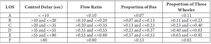
Table 3
LOS Criteria Based on Control Delay and Flow Ratio
LOS Control Delay (sec) Flow Ratio Proportion of Bus Proportion of Three Wheeler
A < =10 <0.10 <0.07 <0.11
B >10 and <=20 >0.10 and <=0.20 >0.07 and <=0.13 >0.11 and <=0.23 C >20 and <=35 >0.20 and <=0.35 >0.13 and <=0.23 >0.23 and <=0.40 D >35 and <=55 >0.35 and <=0.55 >0.23 and <=0.37 >0.40 and <=0.63 E >55 and <=80 >0.55 and <=0.80 >0.37 and <=0.53 >0.63 and <=0.92
F >80 >0.80 >0.53 >0.92
From the delay values obtained from the simulation model,it was observed that it is very difficult to attain LOS A or B in a mixed traffic under saturation condition. So, as to attain the desired LOS at the signalised intersection, proper design of signal timings is to be made. Adequate flow ratio with the required proportion of vehicles should be maintained, which ultimately improves the operating characteristics of the entire traffic stream.
8. Conclusion
The effect of traffic composition on delay, in a single vehicle only condition and also with car and either two wheeler, three wheeler and bus combination were analysed. For analysing the delay variation by varying the traffic composition in a mixed traffic condition, a delay model was developed with total average delay per vehicle as dependant variable and proportions of vehicles as independent variables which provides good statistical results. From the results obtained,
it was clear that the delay gets varied with the proportion of vehicles in the traffic stream and shows that flow ratio played an important role in the variation of delay. The influence of the proportion of vehicles on the flow ratio was also analysed. As bus and three wheelers are considered as the commonly adopted public modes of transport, this also results as a major constituent for increasing the delay in an urban environment.
each LOS, the corresponding flow ratio in par with the delay was estimated. Thus an LOS criteria for a mixed traffic condition was suggested based on control delay and flow ratio as well as proportion of three wheelers and proportion of buses.
References
Akgungor, A. P. 2008. A New Delay Parameter Dependent on Variable Analysis Periods at Signalized Intersections, Part 1: Model development, Transport
23(1): 31-36.
Al-Kubaisi, M. I. 2012. Optimum Cycle Time Prediction for Signalised Intersections at Baghdad City, Conkaya
University Journal of Sciences and Engineering 9(2):
149-166.
Arasan, V. T.; Jagadeesh, K. 1995. Effect of Heterogeneity of Traffic on Delay at Signalized Intersections, Journal
of Transportation Engineering 121(5): 397-404.
Benekohal, R. F.; El-Zohairy, Y. M. 1993. Progression Adjustment Factors for Uniform Delay at Signalized Intersections, Transportation Research Record 1678(5): 32-41.
Bhuyan, P. K.; Rao, K. V. 2011. Application of GPS and Clustering Techniques in Defining LOS Criteria of Signalised Intersections for Indian Cities, Highway
Research Journal, Indian Roads Congress, New Delhi,
4(1): 69-75.
Das, A. K.; Patnaik, A. K.; Dehury, A. N.; Bhuyan, P. K.; Chittaraj, U.; Panda, M. 2013. Defining LOS Criteria for Urban Streets using Neural Gas Clustering, IOSR Journal of Engineering 3(5): 18-25.
Dion, F.; Rakha, H.; Kang, Y. S. 2004. Comparison of delay estimates at under Saturated and Over Saturated Pre-timed Signalized Intersections, Transportation Research: Part B 38(2): 99-122.
Fu, L.; Hellinga, B. 2000. Delay Variability at Signalized Intersections, Transportation Research Record 1710: 215-221.
Highway Capacity Manual 2010, Transportation
Research Board, National Research Council, Washington D.C.
Hoque, S. Md.; Imran, A. Md. 2007. Modification of Webster’s Delay Formulae under Non lane Based Heterogeneous Road Traffic Condition, Journal of Civil
Engineering 35(2): 81-92.
Kumar, P. R.; Dhinakaran, G. 2012. Estimation of Delay at Signalised Intersections for Mixed Traffic Conditions of a Developing Country, International Journal of Civil
Engineering, Transaction A: Civil Engineering 11(1):
53-59.
Minh, C. C.; Binh, T. H.; Mai, T. T.; Kazushi, S. A. N. O. 2009. The Delay Estimation under Heterogeneous Traffic Conditions, Journal of Eastern Asia Society for
Transportation Studies 8(2010): 1583-1595.
Mulandi, J.; Martin, P. T. 2011. Modifications to the Incremental Queue Accumulation Method for Complex Left Turn Phasing, Journal of Basic and Applied Scientific
Research 1(3): 252-259.
Sazi Murat, Y.; Baskan, O. 2006. Modelling Vehicle Delays at Signalized Junctions: Artificial Neural Networks Approach, Journal of Scientific and Industrial
Research 65(7): 558-564.
Olszewski, P. 1993. Overall Delay, Stopped Delay, and Stops at Signalised Intersections, Journal of
Transportation Engineering 119(6): 835 -852.
Sheela, A.; Isaac, K.P. 2014.Traffic simulation model and its application for estimating saturation flow at signalised intersection, International Journal for Traffic
Sheela, A.; Isaac, K.P. 2015. Dynamic PCU Values at signalised intersections in India for mixed traffic, International Journal for Traffic and Transport Engineering, 5(2): 197-209.
Strong, D. W.; Rouphail, N. M. 2006. New Calculation Method for Existing and Extended HCM Delay Estimation Procedure, Paper 06-0107, Proceedings of the 85th Annual Meeting of the Transportation Research
Board, Washington D.C.
Su, Y., Wei, Z., Cheng, S., Yao, D., Zhang, Y.; Li, L. 2009. Delay estimates of Mixed Traffic Flow at Signalised Intersections in China, Tsinghua Science and Technology 14(2): 157-160.