ISSN 2291-8639
Volume 3, Number 1 (2013), 1-13 http://www.etamaths.com
EXPONENTIAL DECAY AND NUMERICAL SOLUTION FOR A TIMOSHENKO SYSTEM WITH DELAY TERM IN THE
INTERNAL FEEDBACK
C. A. RAPOSO1,∗, J. A. D. CHUQUIPOMA1, J. A. J. AVILA1, M. L. SANTOS2
Abstract. In this work we study the asymptotic behavior ast→ ∞of the solution for the Timoshenko system with delay term in the feedback. We use the semigroup theory for to prove the well-posedness of the system and for to establish the exponential stability. As far we know, there exist few results for problems with delay, where the asymptotic behavior is based on the Gearhart-Herbst-Pruss-Huang theorem to dissipative system. See [4],[5],[6]. Finally, we present numerical results of the solution of the system.
1. Introduction
In this paper we consider the following Timoshenko system
ρ1φtt(x, t)−K(φx+ψ)x(x, t) +µ1φt(x, t) +µ2φt(x, t−τ) = 0,
(1)
ρ2ψtt(x, t)−bψxx(x, t) +K(φx+ψ)(x, t) +µ3ψt(x, t) +µ4ψt(x, t−τ)
= 0, (2)
whereφis the transverse displacement of the beam,ψ is the rotation angle of the filament of the beam, (x, t) ∈ (0, L)×(0,∞), τ > 0 represents the time delay and ρ1, ρ2, b, K, µi, i = 1,2,3,4, are positive constants. This beam, of lengthL is subjected to the following boundary conditions
φ(0, t) =φ(L, t) =ψ(0, t) =ψ(L, t) = 0, t >0, (3)
and initial conditions (φ0, φ1, ψ0, ψ1, f0, g0) belongs to a suitable functional space,
defined for allx∈(0, L) by
φ(x,0) =φ0(x), φt(x,0) = φ1(x),
ψ(x,0) =ψ0(x), ψt(x,0) = ψ1(x),
(4)
and for (x, t)∈(0, L)×[0, τ], that implies past history witht−τ≤0, by
φt(x, t−τ) =f0(x, t−τ), ψt(x, t−τ) = g0(x, t−τ).
(5)
Note thatf0(x,0) =φ1(x) andg0(x,0) =ψ1(x).
In the study of the asymptotic behavior, we use the result due to Gearhart. See [4, 5, 6].
2010Mathematics Subject Classification. 35B40, 93D15.
Key words and phrases. Timoshenko system; weak damping; exponential decay; delay.
c
⃝2013 Authors retain the copyrights of their papers, and all open access articles are distributed under the terms of the Creative Commons Attribution License.
Theorem 1.1. Let S(t) = eAt be a C0−Semigroup of contractions on a Hilbert space. ThenS(t)is exponentially stable if and only if
ρ(A)⊇iβ, β∈R (6)
and
lim |β|→∞||
(iβI− A)−1||<∞ (7)
hold.
Certainly, this approach is very different from other works in the literature, espe-cially for problems with delay, where the exponential decay is made by the method of energy, see, for example [8, 9, 10], and references therein. The method of energy, in general, imposes a additional condition on the wave speeds, that is,Kρ2=bρ1,
see [1, 2, 3]. Here we do not use any additional condition for the coefficients of the system. Our work improves the result obtained in [7] in the sense that delays has been introduced in the control ( damping terms ). The delays µ2φt(x, t−τ),
µ4ψt(x, t−τ) makes the problem different from that considered in the literature.
It is well known that small delays in the controls might turn such well-behaving system into a wild one. In recent years, the PDEs with time delay effects have become an active area of research.
The plan of this work is follows: in the next section, we introduce the Energy Space and prove that the full energy of the system decay. In the section 3, we introduce the semigroup representation for the system and prove thatAthe infin-itesimal generator of the semigroup is dissipative, and more, that A generates a eAt,C
0-semigroup of contractions, that implies, prove the existence and regularity
of solution. Finally in the section 4 by Theorem of Gearhart we prove thateAt is exponentially stably.
2. Energy Space
For the Sobolev spaces we use the standard notation as in [11]. Let us proceed as [12]. We introduce the followings new dependents variables as in
z(x, ρ, t) =φt(x, t−τ ρ), w(x, ρ, t) =ψt(x, t−τ ρ), ρ∈(0,1), (8)
that satisfies for (x, ρ, t)∈(0, L)×(0,1)×(0,∞)
τ zt(x, ρ, t) +zρ(x, ρ, t) = 0, τ wt(x, ρ, t) +wρ(x, ρ, t) = 0. (9)
Therefore, problem (1)-(2) is equivalent to
ρ1φtt(x, t)−K(φx+ψ)x(x, t) +µ1φt(x, t) +µ2z(x,1, t) = 0,
ρ2ψtt(x, t)−bψxx(x, t) +K(φx+ψ)(x, t) +µ3ψt(x, t) +µ4w(x,1, t)
= 0, (10)
The above system subjected to the following initial and boundary conditions
φ(0, t) =φ(L, t) =ψ(0, t) =ψ(L, t) = 0, t >0,
z(x,0, t) =φt(x, t), w(x,0, t) =ψt(x, t), x∈(0, L), t >0,
φ(·,0) =φ0, φt(·,0) =φ1, x∈(0, L),
(11)
ψ(·,0) =ψ0, ψt(·,0) =ψ1, x∈(0, L),
z(x,1,0) =f0(x, t−τ), w(x,1,0) =g0(x, t−τ), in (0, L)×(0, τ).
Now, the energy spaceHis defined as
H={H10×L2×H10×L2×L2(0,1; L2)×L2(0,1; L2)}.
Forµ1> µ2,µ3> µ4 satisfying
τ µ2< ξ < τ(2µ1−µ2), τ µ4< η < τ(2µ3−µ4)
(12)
respectively, we define the full energy of the system in the energy space as
E(t) = 1 2
∫ L
0
(ρ1|φt|2+ρ2|ψt|2+K|φx+ψ|2+b|ψx|2)dx
+ ξ 2
∫ L
0
∫ 1
0
z2(x, ρ, t)dρ dx+η 2
∫ L
0
∫ 1
0
w2(x, ρ, t)dρ dx.
Lemma 2.1. There exists a positive constantC such that for any regular solution
(φ, ψ, z, w)of the problem (10)-(11) and for anyt≥0, we have
d
dtE(t)≤ −C
∫ L
0
(|φt|2+|ψt|2+z2(x,1) +w2(x,1))dx. (13)
Proof. 2.1. We multiplying(1) byφt,(2) byψt, and using integration by part to get
1 2
d dt
∫ L
0
(ρ1|φt|2+ρ2|ψt|2+K|φx+ψ|2+b|ψx|2)dx= − µ1
∫ L
0
|φt|2dx
− µ2
∫ L
0
φtz(1, t)dx
− µ3
∫ L
0
|ψt|2dx
− µ4
∫ L
0
ψtw(1, t)dx
and using the Energy E(t)of the system, we obatin
d
dtE(t) =−µ1
∫ L
0
|φt|2dx−µ2
∫ L
0
φtz(1, t)dx− d dt
{
ξ 2
∫ L
0
∫ 1
0
z2(x, ρ, t)dρ dx
}
−µ3
∫ L
0
|ψt|2dx−µ4
∫ L
0
ψtw(1, t)dx− d dt
{
η 2
∫ L
0
∫ 1
0
w2(x, ρ, t)dρ dx
using (14) and (15) d dt ξ 2 ∫ L 0 ∫ 1 0
z2(x, ρ, t)dρ dx = −ξ τ
∫ L
0
∫ 1
0
z(x, ρ, t)zρ(x, ρ, t)dρ dx
= − ξ 2τ ∫ L 0 ∫ 1 0 ∂ ∂ ρz
2(x, ρ, t)dρ dx
= ξ 2τ
∫ L
0
(z2(x,0)−z2(x,1))dx (14) d dt η 2 ∫ L 0 ∫ 1 0
w2(x, ρ, t)dρ dx = −η τ
∫ L
0
∫ 1
0
w(x, ρ, t)wρ(x, ρ, t)dρ dx
= − η 2τ ∫ L 0 ∫ 1 0 ∂ ∂ ρw
2(x, ρ, t)dρ dx
= η 2τ
∫ L
0
(w2(x,0)−w2(x,1))dx (15)
we obtain
d
dtE(t) =−µ1
∫ L
0
|φt|2dx−µ2
∫ L
0
φtz(1, t)dx (16)
+ ξ 2τ
∫ L
0
(z2(x,0)−z2(x,1))dx
−µ3
∫ L
0
|ψt|2dx−µ4
∫ L
0
ψtw(1, t)dx
+η 2τ
∫ L
0
(w2(x,0)−w2(x,1))dx (17)
Now, using Youngs’s inequality we can rewritten the last equation as
d
dtE(t)≤ −
(
µ1−
ξ 2τ −
µ2
2
) ∫ L
0
|φt|2dx−
(
ξ 2τ −
µ2
2
) ∫ L
0
z2(x,1)dx
−(µ3−
η 2τ −
µ4
2
) ∫ L
0
|ψt|2dx−
( η
2τ − µ4
2
) ∫ L
0
w2(x,1)dx
from where our conclusion holds.
3. Existence of solution
Let us introduce the semigroup representation. To this end, letU = (φ, φt, ψ, ψt, z, w)T and rewrite the problem (10)-(11) as
Ut=AU
U(0) =U0
where the operatorAis defined for U = (φ, u=φt, ψ, v=ψt, z, w)T by
AU =
u K
ρ1(φx+ψ)x−
µ1
ρ1u−
µ2
ρ1z(·,1)
v b
ρ2ψxx−
K
ρ2(φx+ψ)−
µ3
ρ2u−
µ4
ρ2w(·,1)
−1 τzρ −1 τwρ , with domain
D(A) ={(φ, φt, ψ, ψt, z, w)T ∈H : u=z(·,0,·), v=w(·,0,·), in(0,1)},
where forx∈(0, L) we denote H = H(0, L), L = L(0, L) and
H ={(H2∩H10)×H10×(H2∩H10)×H10×L2(0,1; H1)×L2(0,1; H1)}.
For U = (φi, ui, ψi, vi, zi, wi)T ∈ H, i = 1,2 and ξ, η as in (12) we defined the following inner product in the energy space as
⟨U1, U2⟩ =
∫ L
0
[ρ1u1u2+ρ2v1v2+K(φ1+ψ1)(φ2+ψ2) +bψ1ψ2)dx
+ ξ
∫ L
0
∫ 1
0
z1(x, ρ)z2(x, ρ)dρ dx+η
∫ L
0
∫ 1
0
w1(x, ρ)w2(x, ρ)dρ dx.
For to prove the existence of solution we begin with the proof that the operatorA is dissipative.
Lemma 3.1. ForU = (φ, u=φt, ψ, v=ψt, z, w)T ∈D(A), we have⟨AU, U⟩ ≤0. Proof. 3.1.
⟨AU, U⟩=−µ1
∫ L
0
|φt|2dx−µ2
∫ L
0
φtz(1, t)dx− ξ τ
∫ L
0
∫ 1
0
z(x, ρ, t)zρ(x, ρ, t)dρ dx
−µ3
∫ L
0
|ψt|2dx−µ4
∫ L
0
ψtw(1, t)dx−η τ
∫ L
0
∫ 1
0
w(x, ρ, t)wρ(x, ρ, t)dρ dx.
Using (14) and (15) in the equation above we obtain
⟨AU, U⟩=−µ1
∫ L
0
|φt|2dx−µ2
∫ L
0
φtz(1, t)dx+ ξ 2τ
∫ L
0
(z2(x,0)−z2(x,1))dx
−µ3
∫ L
0
|ψt|2dx−µ4
∫ L
0
ψtw(1, t)dx+ η 2τ
∫ L
0
(w2(x,0)−w2(x,1))dx.
Now using (16) and Lemma 3.1 we concludes
⟨AU, U⟩= d
dtE(t)≤ −C
∫ L
0
(|u|2+|v|2+z2(x,1) +w2(x,1))dx. (19)
In the next lemma, we will prove an important property of resolvent of the operatorA.
Proof. 3.2. For anyF = (f1, f2, f3, f4, f5, f6)T ∈ Hconsider the equation AU =
F. This implies
u = f1,
(20)
K(φx+ψ)x−µ1u−µ2z(·,1) = ρ1f2,
(21)
v = f3,
(22)
bψxx−K(φx+ψ)−µ3v−µ4w(·,1) = ρ2f4,
(23)
−zρ = τ f5,
(24)
−wρ = τ f6,
(25)
We plugu=f1 obtained from (20) into (21) to get
K(φx+ψ)x=µ1u+µ2z(·,1) +ρ1f2 ∈L2(0, L).
By Poincar`e inequality we have
K(φx+ψ) ∈L2(0, L). (26)
Now we plugv=f3 obtained from (26) and (22) into (23) to get
bψxx=K(φx+ψ) +µ3v+µ4w(·,1) +ρ2f4 ∈L2(0, L).
(27)
By the standard theory in the linear elliptic equations , we have a unique ψ ∈ H2∩H01 satisfying (27). Then we plugψ just obtained from solving (27) into (21) to get
Kφxx=−Kψx+µ1u+µ2z(·,1) +ρ1f2 ∈L2(0, L).
(28)
Applying the standard theory in the linear elliptic equations again yields a unique solvability ofφ∈H2∩H01 for (28).
From (24) we have using Poincar`e inequality,
1 Cp
∫ L
0
∫ 1
0
|z|2dρdx≤
∫ L
0
∫ 1
0
|zρ|2dρdx∈L2(0,1 :L2(0, L)),
then z ∈L2(0,1 : H1(0, L)). The same idea we use for w. Thus the unique solv-ability ofAU =F follows. It is clear from the theory of the linear elliptic equation, see Chapter 1 of[13], that ||U||H≤C||F||H with C being a positive constant inde-pendent ofU, and then0∈ρ(A).
Now we will to prove thatAgenerates aC0−Semigroup of contractions.
Lemma 3.3. The operator A generates a C0−Semigroup of contractions on a Hilbert spaceH.
Proof. 3.3. From Lemma 3.1 we have that A is dissipative operator, and from Lemma 3.2 follows that 0 ∈ ρ(A), them from Theorem 1.2.4, page 3 of [13], we concludes thatA generates aC0−Semigroup of contractions onH.
In this step, we prove that the problem (10)-(11) is well-posedness, and in this direction, we have the following result
Theorem 3.4. If µ2 ≤µ1 and µ4 ≤µ3, then there exists a unique solution U ∈
C([0,∞),H)of the (10)-(11). Moreover ifU0∈D(A), thenU ∈C([0,∞), D(A))∩
Proof. 3.5. From the classical semigroup theory, see for example[14], follows by Lemma 3.3 thatU(t) =eAtU0 is the unique solution of the problem (10)-(11) in the conditions of theorem. The proof is complete.
4. Asymptotic behavior
Now we are in position to present our principal result
Theorem 4.1. The semigroup eAt is exponentially stably.
Proof. 4.2. We now use Theorem 1.1 and we use a contradiction argument. We first prove (6). From Lemma 3.2 we have that0∈ρ(A)and follows from this fact and the contraction mapping theorem that for any real numberβ with|β|<||A||−1,
the operator iβI− A=A(iβA−1−I)is invertible. Moreover,||(iβI− A)−1||is a continuous function of β in the interval(−||A||−1,||A||−1).
If sup{||(iβI− A)−1|| : |β| <||A||−1} =M < ∞, then by the contraction map-ping theorem, the operatoriβI− A= (iβ0I− A)(I+i(β−β0)(iβ0I− A)−1)with |β0|<||A||−1 is invertible for |β−β0|<1/M.It turns out that by choosing|β0|as close to ||A||−1 as we can, we conclude that
{β : |β|<||A||−1+ 1/M} ⊂ρ(A)
and||(iβI− A)−1|| is continuous function of β in the interval
(−||A||−1−1/M , ||A||−1+ 1/M).
From argument above, it follows that if (6) is not true, then there is w∈ R with ||A||−1≤ |w|<∞such that {iβ;|β|<|w|} ⊂ρ(A)and
sup{||(iβ− A)−1|| : |β|<|w|}=∞.
It turns out that there exists a sequence βn ∈ R with βn → w,|βn| < |w| and a
sequence of complex vector functionsUn= (φn, un, ψn, vn, zn, wn)T satisfying
Un ∈D(A) with ||Un||H= 1
such that
||(iβn− A)Un|| →0, asn→ ∞,
and then
iβnφn−un →0 in H10 (29)
iβnρ1un−K(φnx+ψ n)x+µ
1un+µ2zn(·,1)→0 in L2
iβnψn−vn →0 in H10 (30)
iβnρ2vn−bψnxx+K(φ n x+ψ
n) +µ
3vn+µ4wn(·,1)→0 in L2
iβnτ zn−znρ →0 in L2(0,1; L2) iβnτ wn−wnρ →0 in L2(0,1; L2)
Making the inner product of(iβnI− A)Un with Un inH, taking the real part, and
using (19) we have
∫ L
0
from where follows that
un→0 (31)
vn→0 (32)
zn→0 (33)
wn→0 (34)
Using (31) into (29) we obtain
φn →0, (35)
and using (32) into (30) we obtain
φn →0. (36)
Now using (31),(32),(33),(34),(35),(36) we concludes that ||Un|| → 0 which is a
contradiction with ||Un||= 1and the proof of (6) is complete.
Finally we prove (7) by a contradiction argument again. Suppose that (7) is not true. Then there exists a sequence βn with |βn| → ∞ and a sequence of complex vector functionsUn∈D(A)with unit norm inHsuch that
||(iβnI− A)Un|| →0, asn→ ∞.
Again we have
∫ L
0
(|un|2+|vn|2+zn(x,1)2+wn(x,1)2)dx=−⟨AUn, Un⟩ →0. (37)
Making the inner product of (iβnI− A)Un withUn inHwe obtain iβn||Un||2− ⟨AUn, Un⟩ →0.
From (37) we get
βn||Un||2→0. (38)
Asβn → ∞and||Un|| is limited, we concludes that (38) is true only if||Un|| →0 contradict||Un||= 1.The proof of theorem is complete.
5. Numerical Solution
We will solve numerically the system of Timoshenko (1)-(5) in the one-dimension domain Ω of the lengthL, using high-order schemes. We used the Implicit Compact Finite Difference Method of fourth-order for discretization of spacial variable and the classic Finite Difference for discretization of temporal variable.
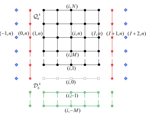
5.1. Discretization. In order to get the discretization of the problem (1)-(5), we define the following sets:
Ωh = {xi: xi=ih, i= 0,1, ... , I+ 1; h=L/(I+ 1)},
⊤k = {tn: tn =nk, n= 0,1, ..., N; k=Ch},
†k
= {tn: tn =nk, n=−M,−M + 1, ...,0; 0< M < N}
where Qkh = Ωh× ⊤k andDkh = Ωh× †k are the computational mesh, and mesh of delay, respectively. The width of meshDk
h is τ =M k. In Figure 1 we show a mesh model for the full-domain Qk
h∪ D k
( ,1)
i
( ,
i N
)
(1, )
n
( , )
I n
( ,0)
i
( 1, )
-
n
(0, )
n
( , )
i n
(
I
+
1, )
n
(
I
+
2, )
n
( , 1)
i
-( ,
i
-
M
)
( ,
i M
)
k h
Q
k hD
Figure 1. Model mesh for the full-domain: Qkh∪ D
k h.
the mesh and, usually denote by (i, n). The classification of nodes is as follows: interiors (circles), boundaries (stars), initials (squares) and ghosts (diamonds).
Letχ=χ(x, t) be a function with second order partial derivatives. Henceforth consider the following notationχn
i ≡χ(xi, tn). We define the following approxima-tion of the derivatives ofχ, according to Taylor,
(χt)ni ≈ 1 kδ
− t χ
n i, (χt)
n i ≈ 1 2kδ 0 tχ n
i, (χt)
(n−M)
i ≈
1 kδ
− t χ
(n−M)
i
(χx)ni ≈ 1 2hδ
0
xχ n
i, (χtt)ni ≈ 1 k2δ
2
tχ n
i, (χxx)ni ≈ 1 h2
[
δ2
x 1 + 1
12δ 2
x
]
χni (39)
where thefinite difference operators are given by
δt−χni :=χni −χni−1, δt0χni :=χin+1−χni−1,
δt−χ(in−M):=χi(n−M)−χi(n−M)−1, δ0xχni :=χni+1−χni−1, δt2χni :=χni+1−2χni +χni−1, δ2xχni :=χni+1−2χni +χni−1,
(40)
[
1 + 1 12δ
2
x
]
χni := 1 12χ
n i+1+
5 6χ n i + 1 12χ n i−1
The discrete formulation of equations (1)-(5) is obtained using (39),
ρ1
[
1 + 1 12δ
2
x
]
δ2tφni −α1δx2φ n i −α2
[
1 + 1 12δ
2
x
]
δx0ψin +
α3
[
1 + 1 12δ
2
x
]
δt0φni +α4
[
1 + 1 12δ
2
x
]
δt−φ(in−M) = 0
ρ2
[
1 + 1 12δ
2
x
]
δt2ψin−β1δx2ψ n i +β2
[
1 + 1 12δ
2
x
]
δ0xφni +β0
[
1 + 1 12δ
2
x
]
ψni +
β3
[
1 + 1 12δ
2
x
]
δ0tψni +β4
[
1 + 1 12δ
2
x
]
δt−ψi(n−M) = 0
in (xi, tn)∈ Qkh (42)
(43) φ0i = (φ0)i, ψ0i = (φ0)i, (φt)i0= (φ1)i, (ψt)0i = (ψ1)i in xi ∈˚Ωh
(44) φn0 =φnI+1=ψn0 =ψnI+1= 0 on tn ∈ ⊤k
(45) φ(in−M)= (f0) (n−M)
i , ψ
(n−M)
i = (g0) (n−M)
i , in (xi, t(n−M))∈ Dkh where, the parameters, are defined by
α1=Kk2/h2, α2=Kk2/2h, α3=µ1k/2, α4=µ2k,
β1=bk2/h2, β2=α2, β0=Kk2, β3=µ3k/2, β4=µ4k
Substituting (40) in (41)-(42), we have the following linear algebraic system:
A1Φn+1 = B1Φn+C1Ψn+D1Φn−1−E1δt−Φ(n−M)+ Υn1
(46)
A2Ψn+1 = B2Ψn+C2Φn+D2Ψn−1−E2δt−Ψ
(n−M)+ Υn
2
(47)
where, Φn+1 = (φn+1 1 , φ
n+1 2 , ..., φ
n+1
I )
T and Ψn+1 = (ψn+1 1 , ψ
n+1 2 , ..., ψ
n+1
I )
T, n=
0,1, ..., N−1, are unknown vectors,
A1= tridiag
(1
12(ρ1+α3), 5
6(ρ1+α3), 1
12(ρ1+α3)
)
,
B1= tridiag
(1
6(ρ1+ 6α1), 1
3(5ρ1−6α1), 1
6(ρ1+ 6α1)
)
,
C1= pentadiag
(
− 1
12α2,− 5 6α2,0,
5 6α2,
1 12α2
)
,
D1= tridiag
( 1
12(−ρ1+α3), 5
6(−ρ1+α3), 1
12(−ρ1+α3)
)
,
E1= tridiag
( 1
12α4, 5 6α4,
1 12α4
)
,
A2= tridiag
(1
12(ρ2+β3), 5
6(ρ2+β3), 1
12(ρ2+β3)
)
,
B2= tridiag
( 1
12(2ρ2+ 12β1−β0), 1
6(10ρ2−12β1−5β0), 1
12(2ρ2+ 12β1−β0)
)
,
C2=−C1,
D2= tridiag
(1
12(−ρ2+β3), 5
6(−ρ2+β3), 1
12(−ρ2+β3)
)
,
E2= tridiag
(1
12β4, 5 6β4,
1 12β4
)
,
are matrices of orderI×I. Υn
1 and Υn2 are vectors of orderIthat load the boundary
5.2. Numerical test. In order to verify the asymptotic behavior of the solution of the Timoshenko system, we consider the following data:
L= 2π, ρ1=ρ2=K=b= 1.
Boundary condition:
φ(0, t) =φ(2π, t) =ψ(0, t) =ψ(2π, t) = 0
Initial condition:
φ0(x) = 0, ψ0(x) = 0, φ1(x) = sin(x), ψ1(x) = cos(x)
Delay condition:
f0(x, t−τ) = sin(x) cos(t−τ), g0(x, t−τ) = cos(x) cos(t−τ)
Numerical data: I = 18, C = 0.3, τ = 10% of the width of the mesh Qkh, T OL= 4×10⁻⁵(tolerance).
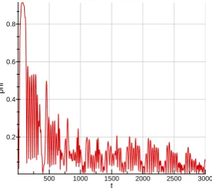
Table 1 shows seven cases where Timoshenko system may behave differently with the presence the terms of delay and damping. Each of these cases are plotted in Figure 2-8. Note that the asymptotic behavior of the solution was calculated by taking the maximum value of the function φ, inx∈ [0,2π], throughout time. In Figure 2, it is observed that there is no asymptotic behavior of the solution, in contrast to Figures 3-6, where the asymptotic behavior of the solution is increasingly more acute. Figure 7 represents the case without delay, the presence of damping is very evident, obtaining the asymptotic behavior of the solution immediately. Figure 8 represents the case without delay and damping, and as was expected, there is no convergence of the solution. In Figure 9 we show the graph of function φ(x, t), where x∈ [0,2π], t ∈[−2.97,29.76], µ1 =µ3 = 1, µ2 = µ4 = 0.8 and we choose
only 300 iterations along time. With respect to rotation angleψ we observe that it exhibits the same behavior that the functionφ.
Table 1. Table for different cases.
Case Damping Delay Iterations in time Asymptotic be-havior
1 µ1=µ3= 1 µ2=µ4= 1 3000 diverges
2 µ1=µ3= 1 µ2=µ4= 0.9 3000 converges
3 µ1=µ3= 1 µ2=µ4= 0.8 3000 converges
4 µ1=µ3= 1 µ2=µ4= 0.7 3000 converges
5 µ1=µ3= 1 µ2=µ4= 0.6 3000 converges
.. .
6 µ1=µ3= 1 µ2=µ4= 0 159 converges
t
p
h
i
500 1000 1500 2000 2500 3000
0.2 0.4 0.6 0.8 1
Figure 2. Case 1.
t
p
h
i
500 1000 1500 2000 2500 3000
0.2 0.4 0.6 0.8
Figure 3. Case 2.
t
p
h
i
500 1000 1500 2000 2500 3000
0.2 0.4 0.6 0.8
Figure 4. Case 3.
t
p
h
i
500 1000 1500 2000 2500 3000
0.1 0.2 0.3 0.4 0.5 0.6 0.7
Figure 5. Case 4.
t
p
h
i
500 1000 1500 2000 2500 3000
0.1 0.2 0.3 0.4 0.5 0.6
Figure 6. Case 5.
t
p
h
i
50 100 150
0.05 0.1 0.15 0.2 0.25 0.3 0.35 0.4
t
p
h
i
500 1000 1500 2000 2500 3000
0.2 0.4 0.6 0.8 1
Figure 8. Case 7.
x 0
2 4
6
t
0
10 20
30
p
h
i
-1 0 1
Figure 9. Graph
ofφ(x, t).
6. Conclusion
We have demonstrated the well-posedness and asymptotic behavior solution of the Timoshenko system. Thus, it also was obtained numerically the asymptotic behavior of the solution confirming the theory developed.
References
[1] A. Soufyane, A. Wehbe, Exponential stability for the Timoshenko beam by a locally dis-tributed damping, Electron. J. Differ. Equ.29(2003), 1-14.
[2] J. E. M. Rivera, R. Racke, Timoshenko systems with indefinite damping. J. Math. Anal. Appl.341(2008), 1068-1083.
[3] F. Amar-Khodja. A. Benabdallah, J. E. M. Rivera, R. Racke, Energy decay for Timoshenko systems of memory type,J. Differ. Equ.194(2003), 82-115.
[4] L. Gearhart, Spectral Theory for the Contractions Semigroups on Hilbert Spaces. Trans. of the American Mathematical Society .236(1978), 385-349.
[5] F. Huang, Characteristic Conditions for Exponential Stability of the Linear Dynamical Sys-tems in Hilbert Spaces.Annals of Differential Equations.1(1985), 43-56.
[6] J. Pr¨uss, On the Spectrumm ofC0-semigroups. Trans. of the American Mathematical Society 284(1984) 847-857.
[7] C. A. Raposo, J. Ferreira, M. L. Santos, N. N. Castro. Exponential Stability for the Timo-shenko System with two weak Dampings.Applied Mathematics Letters.18 (2010), 535-541. [8] B. Said-Houari, Y. Laskri. A stabilit result of a Timoshenko system with a delay term in the
internal feedback.Applied Mathematics and Computation .217(2010), 2857-2869. [9] C. Abdallah, P. Dorato, J. Benitez-Read, R. Byrne. Delayed Positive Feedback Can Stabilize
Oscillatory System. ACC, San Francisco (1993) 3016-3107.
[10] L. H Suh, Z. Bien. Use of time delay action in the controller designe. IEEE Trans. Autom. Control. 25 (1980) 600-603.
[11] R. A. Adams,Sobolev Spaces,Academic Press, New York, 1975.
[12] S. Nicaise, J. Valein. Stabilization of second order evolution eqaution with unbounded feed-back with delay. ESAIM Control. Optim. Calc. Var.16(2010).
[13] Z. Liu, S. Zheng, Semigroups Associated with dissipative systems, Chapman, New Y & Hallo/CRC, New York, 1999.
[14] A. Pazy, Semigroups of Linear Operators and Applications to Partial Differential Equations.
Springer, New York, 1993.
1
Federal University of S˜ao Jo˜ao del-Rei, 36.307-352, S˜ao Jo˜ao del-Rei - MG, Brazil
2
Federal University of Par´a, 36.307-352, Bel´em - PA, Brazil