Evaporative evolution of a Na– Cl– NO
3– K – Ca– SO
4– Mg– Si brine at 95 ° C:
Experiments and modeling relevant to Yucca Mountain, Nevada
Maureen Alai,a兲Mark Sutton, and Susan Carroll
Lawrence Livermore National Laboratory, Livermore, California 94550
共Received 5 November 2004; accepted 21 April 2005; published 7 June 2005兲
A synthetic Topopah Spring Tuff water representative of one type of pore water at Yucca Mountain, NV was evaporated at 95 ° C in a series of experiments to determine the geochemical controls for brines that may form on, and possibly impact upon the long-term integrity of waste containers and drip shields at the designated high-level, nuclear-waste repository. Solution chemistry, condensed vapor chemistry, and precipitate mineralogy were used to identify important chemical divides and to validate geochemical calculations of evaporating water chemistry using a high temperature Pitzer thermodynamic database. The water evolved toward a complex “sulfate type” brine that contained about 45 mol % Na, 40 mol % Cl, 9 mol % NO3, 5 mol % K, and less than 1 mol % each of SO4,
Ca, Mg,兺CO2共aq兲, F, and Si. All measured ions in the condensed vapor phase were below detection
limits. The mineral precipitates identified were halite, anhydrite, bassanite, niter, and nitratine. Trends in the solution composition and identification of CaSO4 solids suggest that fluorite,
carbonate, sulfate, and magnesium-silicate precipitation control the aqueous solution composition of sulfate type waters by removing fluoride, calcium, and magnesium during the early stages of evaporation. In most cases, the high temperature Pitzer database, used byEQ3/6geochemical code, sufficiently predicts water composition and mineral precipitation during evaporation. Predicted solution compositions are generally within a factor of 2 of the experimental values. The model predicts that sepiolite, bassanite, amorphous silica, calcite, halite, and brucite are the solubility controlling mineral phases. ©2005 American Institute of Physics.关DOI: 10.1063/1.1935432兴
I. INTRODUCTION
Yucca Mountain, NV, is the designated site for a perma-nent geologic repository for high-level nuclear waste in the USA. The current waste package design consists of a double-walled container with an inner barrier of stainless steel, an outer barrier of highly corrosion resistant nickel–chromium– molybdenum alloy, and a titanium alloy drip-shield that cov-ers the containcov-ers. Corrosion resistance and long-term integ-rity of the metal containers and shields are important for the safe disposal of the waste. Characterization of the composi-tional evolution of waters that affect waste package corrosion is necessary. If the site is licensed, the waste packages will be placed in tunnels several hundred meters below the ground surface and above the groundwater table in partially saturated volcanic tuff. Once the waste packages are in place, the repository will heat up due to the thermal energy of the nuclear waste. Although the waste packages will be above the groundwater table, pore water present in rock formations within 共Topopah Spring Tuff兲 and above 共Paintbrush Tuff兲 the repository may come into contact with the metal contain-ers and shields. Additionally, brines may form from the deli-quescence of salts found in dusts deposited on the containers.1In this study we focus on seepage brines formed by the evaporation of pore water at elevated temperature.
One method of evaluating the evolution of a brine is the chemical divide theory, which has been used to describe sa-line lake geochemistry.2–5The chemical divide theory
gener-ally describes the chemical evolution of dilute waters upon evaporation in terms of their equivalent calcium, sulfate, and bicarbonate ratios and is shown in Fig. 1共a兲. The chemical evolution of evaporating water is controlled by the high solubility of salt minerals relative to the moderate solu-bility of calcium sulfate and low solusolu-bility of calcium carbonate minerals. A bicarbonate alkaline brine
共Na– K –CO3– Cl– SO4– NO3兲 forms from dilute waters
with dissolved calcium concentrations that are less than dis-solved carbonate共Ca⬍HCO3+ CO3, equivalent%兲. A sulfate brine with near neutral pH 共Na– K – Mg– Cl–SO4– NO3兲
forms from dilute waters with dissolved calcium concentra-tions that are greater than the dissolved carbonate, but less than the combined dissolved sulfate and carbonate concen-trations共Ca⬍SO4+ HCO3, equivalent%兲. A calcium chloride
brine with near neutral pH 共Na– K –Ca– Mg– Cl– NO3兲
forms from dilute waters with a dissolved calcium concen-tration that is greater than the combined dissolved sulfate and carbonate concentrations 共Ca⬎SO4+ HCO3, equivalent%兲.
The measured compositions of Yucca Mountain pore water vary, but can be generally classified as waters that should evolve toward sulfate and sodium bicarbonate type brines, with a few calcium chloride brines as they evaporate 关Fig. 1共b兲兴.6–8
In Fig. 1, the simple ratios of calcium, sulfate, and car-bonate illustrate the dominant carcar-bonate and sulfate chemical divides that occur as waters evaporate.2,9,10However, Fig. 1 does not show important chemical divides for magnesium, silica, or fluoride, nor does it show the relative amount of these salts to other major ions such as sodium, chloride, and a兲Author to whom all correspondence should be addressed; electronic mail:
nitrate. These are important chemical parameters, because they may mitigate or enhance the corrosiveness of brines at the waste package surfaces. Temperature will also impact the evolution of the pore water. Previous modeling of Yucca Mountain pore water initially within the sulfate brine field at 25 ° C evolved toward calcium chloride brines at 95 ° C, and not toward a sulfate brine as predicted by Fig. 1共a兲.7
Thermodynamic equilibrium codes use a range of seep-age water chemistry, temperature, and relative humidity to model the chemical environment on Yucca Mountain waste package surfaces.1 This requires Pitzer parameters that can account for nonideal solutions at higher ionic strengths and elevated temperatures. Unfortunately, only a few relevant ex-periments are available to validate this modeling approach. The available data consist of evaporation of two bicarbonate type waters modeled after Yucca Mountain J-13 well water and a calcium chloride type water modeled after unsaturated pore water at Yucca Mountain and seawater.1,5
In this paper we focus on the brine chemistry formed by
the evaporation of a synthetic Yucca Mountain sulfate type pore water8 at 95 ° C over a concentration range of 1⫻ to
⬃3500⫻. This study provides additional benchmark data needed to both understand the brines and salts that form upon evaporation of various waters and to validate theEQ3/6
geochemical code and a high temperature Pitzer parameter thermodynamic database currently used by the Yucca Moun-tain Program to model aqueous chemical systems.
II. METHODS
A. Experimental methods
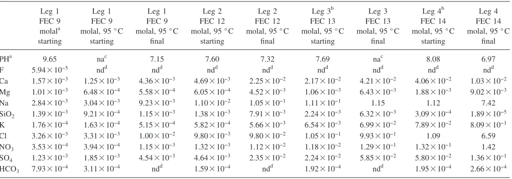
A synthetic pore water solution, based on HD-PERM-1 pore water composition,8was evaporated about 3400 times at 95 ° C in a series of experiments to iteratively concentrate the solution in manageable quantities of approximately 2 l and to monitor precipitation. The chemical composition of each successive leg was based on the brine composition to-ward the end of the previous leg共Table I兲. Experiments FEC
9, 12, 13, and 14 are referred to as legs 1, 2, 3, and 4 throughout this paper. The solutions were prepared at room temperature using analytical grade salts. Differences between the ending and starting compositions for each leg reflect the difficulty in exactly synthesizing the solutions and changes that occur when the solution is prepared at 25 ° C and then heated to the experimental temperature of 95 ° C. At the be-ginning of each new leg, the prepared solution did not in-clude the undissolved solids that were present at the end of the previous leg. During the preparation of the starting solu-tion for legs 3 and 4, an amorphous magnesium silicate pre-cipitate formed in the 25 ° C solutions. This prepre-cipitate was not removed from the starting solutions and only partially dissolved when the solution was heated up to the experimen-tal run temperature共95 ° C兲.
Evaporation was conducted in a vented, halar-lined ves-sel heated to 95 ° C in a fluidized sand bath furnace which provided optimal heat transfer for this method. The solution was stirred constantly and HEPA共high efficiency particulate air兲filtered air was streamed over the solution to help control the evaporation rate. The solution vapor was refluxed to pre-vent evaporative water loss as it was heated to run tempera-ture. Once the solution was at 95 ° C, the evolving water vapor was condensed into a separate container to monitor the extent of evaporation. Samples of the evaporating solution were periodically extracted and filtered at 95 ° C and ana-lyzed to determine the water chemistry. The 95 ° C filtered samples withdrawn for cation and anion analysis were im-mediately diluted by directly injecting the sample into a known quantity of room temperature de-ionized water to pre-vent precipitation on cooling. Undiluted samples withdrawn for total dissolved inorganic carbon analysis, 兺CO2共aq兲,
were immediately stored by filling gas tight vials to prevent equilibration with air at room temperature. Separate undi-luted samples for solution pH were stored in a closed con-tainer andpH was measured as soon as they cooled to room temperature. In the last two samples of leg 4, precipitates
formed in the pH and carbon samples as they cooled. Samples of the condensed water vapor were also periodically extracted and analyzed to monitor gas volatility. After the last sample was taken for each leg, the evaporation was con-tinued to dryness. The solid precipitate was collected at the end of each leg of the experiment, dried in an oven at 40 ° C to facilitate sample preparation, and analyzed by powder x-ray diffraction 共XRD兲.
B. Analytical methods
Sample pH was measured at room temperature with a combination electrode, which is reliable in solutions with an ionic strength less than 0.1 molal.11 The sample cooled to room temperature and pH was measured within a half hour of sampling. The pH measurements for legs 3 and 4, where the ionic strength of the solution was greater than 0.1 molal, represent uncorrected values and have not been corrected for ionic strength. Total dissolved carbon,兺CO2共aq兲, was mea-sured with an infrared carbon analyzer and had a detection limit of 1 ppm. Dissolved calcium, magnesium, silica, and sodium were measured with an inductively coupled plasma-atomic emission spectrometer, dissolved potassium was mea-sured using an atomic absorption spectrophotometer, and fluoride, chloride, nitrate, and sulfate anions were deter-mined using ion chromatography. Reproducibility of these techniques is typically better than ±2%. The mineralogical composition was determined by powdered XRD using a Cu K␣ source from 10° to 90° 2 at 0.02° per step. The XRD instrument was calibrated using NIST traceable silicon 共# 640c兲 and mica 共# 675兲 standards for high angle and low angle peaks, respectively. XRD cannot detect amorphous sol-ids or minerals that are present at ⬍2 wt %. Mineral identi-fication was based on the presence of the three most intense peaks in the XRD pattern for a given mineral. In some cases
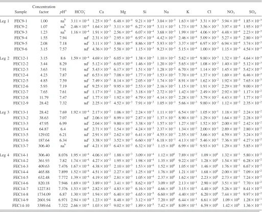
TABLE I. Starting and final compositions for the evaporation of a synthetic “sulfate type” Topopah Spring Tuff pore water.
Leg 1 FEC 9 molala starting
Leg 1 FEC 9 molal, 95 ° C
starting
Leg 1 FEC 9 molal, 95 ° C
final
Leg 2 FEC 12 molal, 95 ° C
starting
Leg 2 FEC 12 molal, 95 ° C
final
Leg 3b FEC 13 molal, 95 ° C
starting
Leg 3 FEC 13 molal, 95 ° C
final
Leg 4b FEC 14 molal, 95 ° C
starting
Leg 4 FEC 14 molal, 95 ° C
final
PHa 9.65 nac 7.15 7.60 7.32 7.69 nac 8.08 6.97
F 5.94⫻10−5 ndd ndd ndd ndd ndd ndd ndd ndd
Ca 1.57⫻10−3 1.25⫻10−3 4.36⫻10−3 4.69⫻10−3 2.25⫻10−2 2.17⫻10−2 4.21⫻10−2 4.06⫻10−2 1.03⫻10−2
Mg 1.01⫻10−3 6.48⫻10−4 5.58⫻10−4 6.05⫻10−4 4.52⫻10−3 1.06⫻10−3 6.43⫻10−3 1.88⫻10−3 9.02⫻10−3
Na 2.84⫻10−3 3.04⫻10−3 9.23⫻10−3 1.10⫻10−2 1.05⫻10−1 1.11⫻10−1 1.15 1.12 7.42
SiO2 1.39⫻10−3 9.21⫻10−4 1.15⫻10−3 1.38⫻10−3 7.91⫻10−3 2.24⫻10−3 6.32⫻10−3 3.09⫻10−4 1.89⫻10−5
K 1.76⫻10−4 1.63⫻10−4 5.15⫻10−4 5.82⫻10−4 5.66⫻10−3 6.54⫻10−3 6.99⫻10−2 7.89⫻10−2 8.09⫻10−1
Cl 3.26⫻10−3 3.31⫻10−3 1.00⫻10−2 9.80⫻10−3 9.80⫻10−2 1.05⫻10−1 9.93⫻10−1 1.09 6.59
NO3 3.53⫻10−4 3.94⫻10−4 1.15⫻10−3 1.32⫻10−3 1.12⫻10−2 1.18⫻10−2 1.29⫻10−1 1.32⫻10−1 1.42
SO4 1.23⫻10−3 1.85⫻10−3 4.54⫻10−3 4.64⫻10−3 2.35⫻10−2 2.24⫻10−2 5.85⫻10−2 5.80⫻10−2 1.36⫻10−1
HCO3 7.93⫻10−4 3.11⫻10−4 ndd 1.59⫻10−4 ndd 1.92⫻10−4 ndd 1.95⫻10−4 2.66⫻10−4
aMeasured at room temperature.
bMagnesium and silica precipitated from the solution at 25 ° C. Initial gravimetric concentrations are Mg= 4.5⫻10−3mol/ kg-solution and Si= 7.8
⫻10−3mol/ kg-solution for Leg3 and are Mg= 6.0⫻10−3mol/ kg-solution and Si= 5.9⫻10−3mol/ kg-solution for Leg4. cNot analyzed.
where the most intense peaks overlapped with other mineral peaks, identification was based on the presence of lower in-tensity diagnostic peaks.
C. Thermodynamic modeling calculations
Solution compositions were modeled using the EQ3/6
geochemical code, and a high temperature Pitzer ion-interaction model that is further described in Table II1,12–14 The high temperature Pitzer ion-interaction model approxi-mates nonideal behavior of solutions at elevated ionic strength and temperature. The predictive models were gener-ated to mirror the experimental design and analysis, in which synthetic pore water was evaporated over a discrete range for each leg, with a cumulative evaporation up to 3500⫻for the overall experiment. The concentration factor, CF, can then be defined as
CF共n兲=
H2O共i兲
H2O共n兲
, 共1兲
where H2O共i兲is the initial mass of H2O solvent and H2O共n兲is
the mass of H2O solvent remaining after thenth step in the
evaporation process.
The evaporation model consisted of three steps. In the first step, the measured composition of the first sample at 95 ° C共Table I, FEC#-1兲was speciated, suppressing all min-eral precipitation in the calculation. At this point in the ex-periment, the solution was simply brought up to temperature, refluxing any water vapor to prevent evaporation. During the second step, the speciated water was evaporated by stepwise removal of solvent water at a fixed rate of 0.25 mol H2O
reactant per mol of solute at 95 ° C. In the evaporation step, all minerals were allowed to precipitate with the exception of quartz and dolomite because of known slow kinetics; glaser-ite, hydromagnesglaser-ite, and magnesite because the available thermodynamic data are questionable; and cristobalite be-cause it forms above 1470 ° C and is not relevant to this experiment. In the speciation and evaporation steps, oxygen and carbon dioxide fugacities were fixed at 21% and 0.033%, respectively, to simulate atmospheric experimental condi-tions. A CO2共g兲-sink was added to the model to remove
ex-cess buildup of CO2共g兲from the reaction surface. Finally, in
the third step, the predictedpH values at 95 ° C were recal-culated to 25 ° C to compare with measured pH at room temperature. This was achieved by performing a further cal-culation that reduced the temperature of the reaction from 95 to 25 ° C, while fixing 兺CO2共aq兲 to the predicted 95 ° C
value and suppressing mineral formation. For all calcula-tions, electrical balance was achieved by automatically changing the sodium concentration with a convergence tol-erance of 0.1 ppb. Charge balancing was necessary due to analytical errors generated in the experimental analysis and also potentially incomplete analysis. The calculated activity of water was interpreted as a function of relative humidity, and predicted solution composition,pH, and mineral compo-sition were compared with experimental ion analysis and XRPD results with respect to the overall concentration fac-tor. The results are shown graphically in Figs. 3 and 4, and discussed in the following sections.
III. RESULTS
Evaporation of the dilute water yielded a sulfate brine as predicted by chemical divide theory based on its initial Ca: SO4: HCO3 ratio共Fig. 2兲. Although this water is
classi-fied as a sulfate brine, sulfate concentrations are minor com-pared to the concentration of sodium and chloride, which dominate the solution chemistry. At the conclusion of leg 4, sodium and chloride were 45 and 40 mol %, respectively, while calcium and sulfate were relatively minor constituents at 0.1 and 0.8 mol %, respectively 共Table III兲. The initial experimental solution contained trace amounts of fluoride that were rapidly removed from solution presumably as highly insoluble fluorite 共CaF2兲 共Table I兲. Fluoride was not
included in the model since it was not detected in the first sample analysis at 95 ° C 共leg 1, FEC9-1兲. The minerals identified by XRD in the precipitates are halite共NaCl兲, bas-sanite 共2CaSO4·H2O兲, anhydrite 共CaSO4兲, niter 共KNO3兲, and nitratine 共NaNO3兲, and are listed for each leg in Table
IV.
We see no evidence of volatility for HCl, HNO3, and HF
gases in these experiments. Concentrations of fluoride, chlo-ride, nitrate, and sulfate in the condensed vapor were all below the detection limits. This is in contrast to evaporation of a concentrated calcium chloride type water at around 140 ° C 共based on the 1000⫻ solution results from Rosen-berg et al.5兲 where significant volatilization of HCl共g兲 was measured by acidic condensates at 90% evaporation at
⬃75 000⫻.15 While our evaporation is less than the afore-mentioned research, our results indicate that gas volatility is not a major concern for the evaporation and concentration of sulfate waters at 95 ° C and⬃3 400⫻.
Figures 3 and 4 show the experimental and predicted solution composition and the predicted mineral precipitation as a function of overall concentration factor. There is excel-lent agreement between the model predictions of potassium and nitrate concentrations with those measured by experi-ment. Solution data show conservative concentration of both potassium and nitrate in each evaporation leg, indicating no mineral precipitation关Figs. 3共a兲and 4兴. This is supported by the XRD data where only a small amount of niter was iden-tified in the last leg after the solution had completely evapo-rated when precipitation of all mineral phases is expected
共Table IV兲. Calculations required the suppression of pentasalt
共gorgeyite, K2Ca5共SO4兲6·H2O兲precipitation at a
concentra-tion factor above 1000⫻in leg 4关Fig. 3共a兲兴to achieve agree-ment with experiagree-mental solution composition and solid char-acterization. Pentasalt was not detected by XRD analysis.
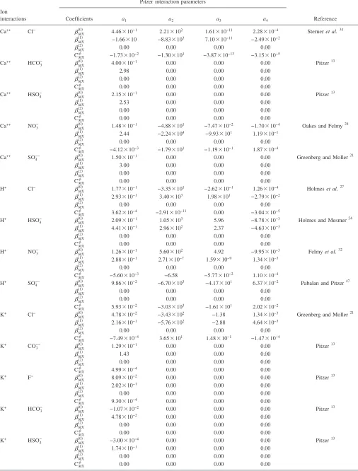
de-TABLE II. Temperature dependence of Pitzer interaction parameters. 25 ° C-centric equation used to derive parameters:共T兲=a1+a2关兵1 /T其−兵1 / 298.15其兴
+a3ln兵T/ 298.15其+a4兵T− 298.15其.
Ion interactions
Pitzer interaction parameters
Reference
Coefficients a1 a2 a3 a4
Ca++ Cl− 
MX
共0兲 4.46⫻10−1 2.21⫻102 1.61⫻10−11 2.28⫻10−4 Sterneret al.34
MX
共1兲 −1.66⫻10 −8.83⫻103 7.10⫻10−11 −2.49⫻10−2
MX
共2兲 0.00 0.00 0.00 0.00
CMX −1.73⫻10−2 −1.30⫻101 −3.87⫻10−13 −3.15⫻10−5
Ca++ HCO
3
− 
MX
共0兲 4.00⫻10−1 0.00 0.00 0.00 Pitzer13
MX
共1兲 2.98 0.00 0.00 0.00
共MX
2兲 0.00 0.00 0.00 0.00
CMX 0.00 0.00 0.00 0.00
Ca++ HSO
4
− 
MX
共0兲 2.15⫻10−1 0.00 0.00 0.00 Pitzer13
共MX
1兲 2.53 0.00 0.00 0.00
MX
共2兲 0.00 0.00 0.00 0.00
CMX 0.00 0.00 0.00 0.00
Ca++ NO
3
− 
MX
共0兲 1.48⫻10−1 −4.88⫻101 −7.47⫻10−2 −1.70⫻10−4 Oakes and Felmy28
MX
共1兲 2.44 −2.24⫻104 −9.93⫻101 1.19⫻10−1
MX
共2兲 0.00 0.00 0.00 0.00
CMX −4.12⫻10−3 −1.79⫻101 −1.19⫻10−1 1.87⫻10−4
Ca++ SO
4
−− 
MX
共0兲 1.50⫻10−1 0.00 0.00 0.00 Greenberg and Moller21
MX
共1兲 3.00 0.00 0.00 0.00
共MX
2兲 0.00 0.00 0.00 0.00
CMX 0.00 0.00 0.00 0.00
H+ Cl− 
MX
共0兲 1.77⫻10−1 −3.35⫻101 −2.62⫻10−1 1.26⫻10−4 Holmeset al.27
共MX
1兲 2.93⫻10−1 3.40⫻103 1.98⫻101 −2.79⫻10−2
MX
共2兲 0.00 0.00 0.00 0.00
CMX 3.62⫻10−4 −2.91⫻10−11 0.00 −3.04⫻10−5
H+ HSO
4
− 
MX
共0兲 2.09⫻10−1 1.05⫻103 5.96 −8.78⫻10−3 Holmes and Mesmer24
MX
共1兲 4.41⫻10−1 2.96⫻102 2.37 −4.63⫻10−3
MX
共2兲 0.00 0.00 0.00 0.00
CMX 0.00 0.00 0.00 0.00
H+ NO
3
− 
MX
共0兲 1.26⫻10−1 5.60⫻102 4.92 −9.95⫻10−3 Felmyet al.32
MX
共1兲 2.88⫻10−1 2.71⫻10−7 1.59⫻10−9 1.34⫻10−3
MX
共2兲 0.00 0.00 0.00 0.00
CMX −5.60⫻10−3 −6.58 −5.77⫻10−2 1.10⫻10−4
H+ SO
4
−− 
MX
共0兲 9.86⫻10−2 −6.70⫻103 −4.17⫻101 6.37⫻10−2 Pabalan and Pitzer47
MX
共1兲 0.00 0.00 0.00 0.00
共MX
2兲 0.00 0.00 0.00 0.00
CMX 5.93⫻10−2 −3.03⫻103 −1.61⫻101 2.02⫻10−2
K+ Cl− 
MX
共0兲 4.78⫻10−2 −3.43⫻102 −1.38 1.34⫻10−3 Greenberg and Moller21
MX
共1兲 2.16⫻10−1 −5.76⫻102 −2.88 4.64⫻10−3
MX
共2兲 0.00 0.00 0.00 0.00
CMX −7.49⫻10−4 3.65⫻101 1.48⫻10−1 −1.47⫻10−4
K+ CO
3
−− 
MX
共0兲 1.29⫻10−1 0.00 0.00 0.00 Pitzer13
MX
共1兲 1.43 0.00 0.00 0.00
MX
共2兲 0.00 0.00 0.00 0.00
CMX 4.99⫻10−4 0.00 0.00 0.00
K+ F− 
MX
共0兲 8.09⫻10−2 0.00 0.00 0.00 Pitzer13
MX
共1兲 2.02⫻10−1 0.00 0.00 0.00
共MX
2兲 0.00 0.00 0.00 0.00
CMX 9.30⫻10−4 0.00 0.00 0.00
K+ HCO
3
− 
MX
共0兲 −1.07⫻10−2 0.00 0.00 0.00 Pitzer13
共MX
1兲 4.78⫻10−2 0.00 0.00 0.00
MX
共2兲 0.00 0.00 0.00 0.00
CMX 0.00 0.00 0.00 0.00
K+ HSO
4
− 
MX
共0兲 −3.00⫻10−4 0.00 0.00 0.00 Pitzer13
MX
共1兲 1.74⫻10−1 0.00 0.00 0.00
MX
共2兲 0.00 0.00 0.00 0.00
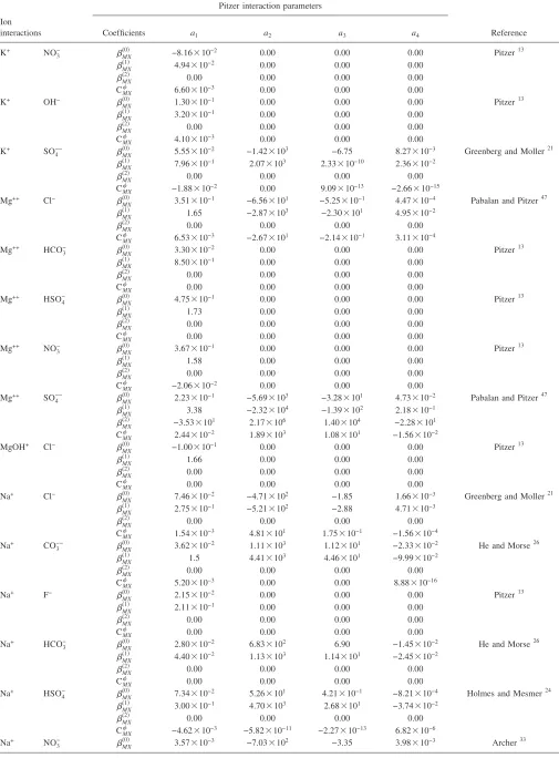
TABLE II. 共Continued.兲
Ion interactions
Pitzer interaction parameters
Reference
Coefficients a1 a2 a3 a4
K+ NO
3
− 
MX
共0兲 −8.16⫻10−2 0.00 0.00 0.00 Pitzer13
MX
共1兲 4.94⫻10−2 0.00 0.00 0.00
MX
共2兲 0.00 0.00 0.00 0.00
CMX 6.60⫻10−3 0.00 0.00 0.00
K+ OH− 
MX
共0兲 1.30⫻10−1 0.00 0.00 0.00 Pitzer13
MX
共1兲 3.20⫻10−1 0.00 0.00 0.00
共MX
2兲 0.00 0.00 0.00 0.00
CMX 4.10⫻10−3 0.00 0.00 0.00
K+ SO
4
−− 
MX
共0兲 5.55⫻10−2 −1.42⫻103 −6.75 8.27⫻10−3 Greenberg and Moller21
共MX
1兲 7.96⫻10−1 2.07⫻103 2.33⫻10−10 2.36⫻10−2
MX
共2兲 0.00 0.00 0.00 0.00
CMX −1.88⫻10−2 0.00 9.09⫻10−13 −2.66⫻10−15
Mg++ Cl− 
MX
共0兲 3.51⫻10−1 −6.56⫻101 −5.25⫻10−1 4.47⫻10−4 Pabalan and Pitzer47
MX
共1兲 1.65 −2.87⫻103 −2.30⫻101 4.95⫻10−2
MX
共2兲 0.00 0.00 0.00 0.00
CMX 6.53⫻10−3 −2.67⫻101 −2.14⫻10−1 3.11⫻10−4
Mg++ HCO
3
− 
MX
共0兲 3.30⫻10−2 0.00 0.00 0.00 Pitzer13
MX
共1兲 8.50⫻10−1 0.00 0.00 0.00
共MX
2兲 0.00 0.00 0.00 0.00
CMX 0.00 0.00 0.00 0.00
Mg++ HSO
4
− 
MX
共0兲 4.75⫻10−1 0.00 0.00 0.00 Pitzer13
共MX
1兲 1.73 0.00 0.00 0.00
MX
共2兲 0.00 0.00 0.00 0.00
CMX 0.00 0.00 0.00 0.00
Mg++ NO
3
− 
MX
共0兲 3.67⫻10−1 0.00 0.00 0.00 Pitzer13
MX
共1兲 1.58 0.00 0.00 0.00
MX
共2兲 0.00 0.00 0.00 0.00
CMX −2.06⫻10−2 0.00 0.00 0.00
Mg++ SO
4
−− 
MX
共0兲 2.23⫻10−1 −5.69⫻103 −3.28⫻101 4.73⫻10−2 Pabalan and Pitzer47
MX
共1兲 3.38 −2.32⫻104 −1.39⫻102 2.18⫻10−1
MX
共2兲 −3.53⫻101 2.17⫻106 1.40⫻104 −2.28⫻101
CMX 2.44⫻10−2 1.89⫻103 1.08⫻101 −1.56⫻10−2
MgOH+ Cl− 
MX
共0兲 −1.00⫻10−1 0.00 0.00 0.00 Pitzer13
MX
共1兲 1.66 0.00 0.00 0.00
共MX
2兲 0.00 0.00 0.00 0.00
CMX 0.00 0.00 0.00 0.00
Na+ Cl− 
MX
共0兲 7.46⫻10−2 −4.71⫻102 −1.85 1.66⫻10−3 Greenberg and Moller21
共MX
1兲 2.75⫻10−1 −5.21⫻102 −2.88 4.71⫻10−3
MX
共2兲 0.00 0.00 0.00 0.00
CMX 1.54⫻10−3 4.81⫻101 1.75⫻10−1 −1.56⫻10−4
Na+ CO
3
−− 
MX
共0兲 3.62⫻10−2 1.11⫻103 1.12⫻101 −2.33⫻10−2 He and Morse26
MX
共1兲 1.5 4.41⫻103 4.46⫻101 −9.99⫻10−2
MX
共2兲 0.00 0.00 0.00 0.00
CMX 5.20⫻10−3 0.00 0.00 8.88⫻10−16
Na+ F− 
MX
共0兲 2.15⫻10−2 0.00 0.00 0.00 Pitzer13
MX
共1兲 2.11⫻10−1 0.00 0.00 0.00
共MX
2兲 0.00 0.00 0.00 0.00
CMX 0.00 0.00 0.00 0.00
Na+ HCO
3
− 
MX
共0兲 2.80⫻10−2 6.83⫻102 6.90 −1.45⫻10−2 He and Morse26
共MX
1兲 4.40⫻10−2 1.13⫻103 1.14⫻101 −2.45⫻10−2
MX
共2兲 0.00 0.00 0.00 0.00
CMX 0.00 0.00 0.00 0.00
Na+ HSO
4
− 
MX
共0兲 7.34⫻10−2 5.26⫻101 4.21⫻10−1 −8.21⫻10−4 Holmes and Mesmer24
MX
共1兲 3.00⫻10−1 4.70⫻103 2.68⫻101 −3.74⫻10−2
MX
共2兲 0.00 0.00 0.00 0.00
CMX −4.62⫻10−3 −5.82⫻10−11 −2.27⫻10−13 6.82⫻10−6
Na+ NO
3
− 
MX
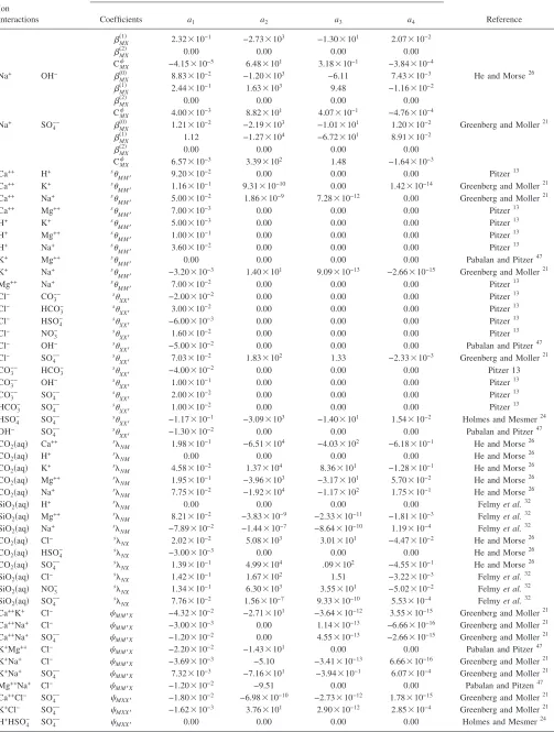
TABLE II. 共Continued.兲
Ion interactions
Pitzer interaction parameters
Reference
Coefficients a1 a2 a3 a4
MX
共1兲 2.32⫻10−1 −2.73⫻103 −1.30⫻101 2.07⫻10−2
MX
共2兲 0.00 0.00 0.00 0.00
CMX −4.15⫻10−5 6.48⫻101 3.18⫻10−1 −3.84⫻10−4
Na+ OH− 
MX
共0兲 8.83⫻10−2 −1.20⫻103 −6.11 7.43⫻10−3 He and Morse26
MX
共1兲 2.44⫻10−1 1.63⫻103 9.48 −1.16⫻10−2
MX
共2兲 0.00 0.00 0.00 0.00
CMX 4.00⫻10−3 8.82⫻101 4.07⫻10−1 −4.76⫻10−4
Na+ SO
4
−− 
MX
共0兲 1.21⫻10−2 −2.19⫻103 −1.01⫻101 1.20⫻10−2 Greenberg and Moller21
MX
共1兲 1.12 −1.27⫻104 −6.72⫻101 8.91⫻10−2
共MX
2兲 0.00 0.00 0.00 0.00
CMX 6.57⫻10−3 3.39⫻102 1.48 −1.64⫻10−3
Ca++ H+ s
MM⬘ 9.20⫻10
−2 0.00 0.00 0.00 Pitzer13
Ca++ K+ s
MM⬘ 1.16⫻10−1 9.31⫻10−10 0.00 1.42⫻10−14 Greenberg and Moller
21
Ca++ Na+ s
MM⬘ 5.00⫻10
−2 1.86⫻10−9 7.28⫻10−12 0.00 Greenberg and Moller21
Ca++ Mg++ s
MM⬘ 7.00⫻10
−3 0.00 0.00 0.00 Pitzer13
H+ K+ s
MM⬘ 5.00⫻10
−3 0.00 0.00 0.00 Pitzer13
H+ Mg++ s
MM⬘ 1.00⫻10−1 0.00 0.00 0.00 Pitzer
13
H+ Na+ s
MM⬘ 3.60⫻10
−2 0.00 0.00 0.00 Pitzer13
K+ Mg++ s
MM⬘ 0.00 0.00 0.00 0.00 Pabalan and Pitzer
47
K+ Na+ s
MM⬘ −3.20⫻10
−3 1.40⫻101 9.09⫻10−13 −2.66⫻10−15 Greenberg and Moller21
Mg++ Na+ s
MM⬘ 7.00⫻10−2 0.00 0.00 0.00 Pitzer
13
Cl− CO
3
−− s
XX⬘ −2.00⫻10
−2 0.00 0.00 0.00 Pitzer13
Cl− HCO
3
− s
XX⬘ 3.00⫻10
−2 0.00 0.00 0.00 Pitzer13
Cl− HSO
4
− s
XX⬘ −6.00⫻10
−3 0.00 0.00 0.00 Pitzer13
Cl− NO
3
− s
XX⬘ 1.60⫻10
−2 0.00 0.00 0.00 Pitzer13
Cl− OH− s
XX⬘ −5.00⫻10
−2 0.00 0.00 0.00 Pabalan and Pitzer47
Cl− SO
4
−− s
XX⬘ 7.03⫻10
−2 1.83⫻102 1.33 −2.33⫻10−3 Greenberg and Moller21
CO3−− HCO
3
− s
XX⬘ −4.00⫻10−2 0.00 0.00 0.00 Pitzer 13
CO3−− OH− s
XX⬘ 1.00⫻10
−1 0.00 0.00 0.00 Pitzer13
CO3−− SO4−− s
XX⬘ 2.00⫻10
−2 0.00 0.00 0.00 Pitzer13
HCO3− SO4−−
s
XX⬘ 1.00⫻10
−2 0.00 0.00 0.00 Pitzer13
HSO4− SO
4
−− s
XX⬘ −1.17⫻10−1 −3.09⫻103 −1.40⫻101 1.54⫻10−2 Holmes and Mesmer
24
OH− SO
4
−− s
XX⬘ −1.30⫻10
−2 0.00 0.00 0.00 Pabalan and Pitzer47
CO2共aq兲 Ca++
s
NM 1.98⫻10−1 −6.51⫻104 −4.03⫻102 −6.18⫻10−1 He and Morse
26
CO2共aq兲 H+ sNM 0.00 0.00 0.00 0.00 He and Morse
26
CO2共aq兲 K+
s
NM 4.58⫻10−2 1.37⫻104 8.36⫻101 −1.28⫻10−1 He and Morse
26
CO2共aq兲 Mg++ sNM 1.95⫻10−1 −3.96⫻103 −3.17⫻101 5.70⫻10−2 He and Morse
26
CO2共aq兲 Na+
s
NM 7.75⫻10−2 −1.92⫻104 −1.17⫻102 1.75⫻10−1 He and Morse26
SiO2共aq兲 H+ sNM 0.00 0.00 0.00 0.00 Felmyet al.
32
SiO2共aq兲 Mg++
s
NM 8.21⫻10−2 −3.83⫻10−9 −2.33⫻10−11 −1.81⫻10−3 Felmyet al.32
SiO2共aq兲 Na+ sNM −7.89⫻10−2 −1.44⫻10−7 −8.64⫻10−10 1.19⫻10−4 Felmyet al.
32
CO2共aq兲 Cl− s
NX 2.02⫻10−2 5.08⫻103 3.01⫻101 −4.47⫻10−2 He and Morse
26
CO2共aq兲 HSO4−
s
NX −3.00⫻10−3 0.00 0.00 0.00 He and Morse
26
CO2共aq兲 SO4−− s
NX 1.39⫻10−1 4.99⫻104 .09⫻102 −4.55⫻10−1 He and Morse
26
SiO2共aq兲 Cl− sNX 1.42⫻10−1 1.67⫻102 1.51 −3.22⫻10−3 Felmyet al.
32
SiO2共aq兲 NO3−
s
NX 1.34⫻10−1 6.30⫻103 3.55⫻101 −5.02⫻10−2 Felmyet al.
32
SiO2共aq兲 SO4
−− s
NX 7.76⫻10−2 1.56⫻10−7 9.33⫻10−10 5.53⫻10−4 Felmyet al.
32
Ca++K+ Cl−
MM⬘X −4.32⫻10−2 −2.71⫻101 −3.64⫻10−12 3.55⫻10−15 Greenberg and Moller21
Ca++Na+ Cl−
MM⬘X −3.00⫻10−3 0.00 1.14⫻10−13 −6.66⫻10−16 Greenberg and Moller21
Ca++Na+ SO 4
−−
MM⬘X −1.20⫻10−2 0.00 4.55⫻10−13 −2.66⫻10−15 Greenberg and Moller21
K+Mg++ Cl−
MM⬘X −2.20⫻10−2 −1.43⫻101 0.00 0.00 Pabalan and Pitzer47
K+Na+ Cl−
MM⬘X −3.69⫻10−3 −5.10 −3.41⫻10−13 6.66⫻10−16 Greenberg and Moller21
K+Na+ SO
4
−−
MM⬘X 7.32⫻10−3 −7.16⫻101 −3.94⫻10−1 6.07⫻10−4 Greenberg and Moller21
Mg++Na+ Cl−
MM⬘X −1.20⫻10−2 −9.51 0.00 0.00 Pabalan and Pitzen47
Ca++Cl− SO 4
−−
MXX⬘ −1.80⫻10−2 −6.98⫻10−10 −2.73⫻10−12 1.78⫻10−15 Greenberg and Moller21
K+Cl− SO
4
−−
MXX⬘ −1.62⫻10−3 3.76⫻101 2.90⫻10−12 2.85⫻10−4 Greenberg and Moller21
H+HSO 4 − SO
4
−−
MXX⬘ 0.00 0.00 0.00 0.00 Holmes and Mesmer
crease in calculated sodium concentration to neutralize the charge discrepancy. The charge balance correction resulted in a sodium concentration that differed from the original共 mea-sured兲 concentration by 21% in the first leg, 13% in the second leg, 1% in the third leg, and 5% in the fourth leg. Since sodium saturation did not occur until the formation of halite late in fourth leg, we believe this sodium correction did not significantly affect the quality of our calculations.
There is also good agreement between experimental compositions and model prediction for calcium and sulfate
关Figs. 3共c兲 and 4兴. At a concentration factor of roughly 10
⫻ in leg 2, both calcium and sulfate begin to precipitate as can be seen in the decrease in their slopes. Although calcium sulfate precipitation continues over the duration of the ex-periment, dissolved calcium decreases as the sulfate
in-creases with continued evaporation at a concentration factor of about 1000⫻. This is consistent with the chemical divide theory and the initial composition of the water which con-tained SO4: Ca⬎1. This behavior was best modeled by using
bassanite as the solubility limiting phase 共using gypsum or anhydrite resulted in an overprediction and underprediction, respectively, of the calcium and sulfate concentrations兲. This finding is in partial agreement with the experiments, which identified both anhydrite and bassanite共Table IV兲. This dif-ference may be an artifact of the experimental protocol be-cause calcium sulfate hydration states can be readily altered by changes in temperature and humidity, such as those found in the drying and preparation of the precipitate prior to XRD analysis. The model overestimates calcium and sulfate by about a factor of 2 in concentrated brines共1000⫻ concentra-tion factor兲, and appears to increase with continued evapora-tion. It is possible that the overprediction in calcium and sulfate concentrations observed using bassanite and gypsum solubility controls, and the underprediction observed with anhydrite controls indicates a metastable mixture of these solubility limiting phases.
Comparison between both magnesium and silica experi-mental concentrations and model predictions during the evaporation show reasonable agreement in legs 2 and 3 and only fair agreement in legs 1 and 4关Fig. 3共f兲兴. Experiment and prediction both show that magnesium and silica are re-moved from solution as solid precipitates. The model pre-dicts that sepiolite, amorphous silica, and brucite are the solubility controls共Fig. 4兲. These phases were not observed in the experiment possibly because the amount was too small to be detected or because they were amorphous. It is possible that a noncrystalline magnesium silicate phase precipitated, similar to the solid that formed at 25 ° C 共Legs 3 and 4兲.16 The Pitzer database contained only two magnesium silicate minerals, talc 共Mg3Si4O10共OH兲2兲 and sepiolite FIG. 2. 共Color兲Chemical evolution of dilute calcium chloride共synthetic
Topopah Spring tuff porewater—Ref. 5兲, Na-bicarbonate 共synthetic J-13 groundwater—Ref. 5兲, and sulfate共synthetic Topopah Spring tuff porewater, this study兲waters upon evaporation.
TABLE II. 共Continued.兲
Ion interactions
Pitzer interaction parameters
Reference
Coefficients a1 a2 a3 a4
Mg++Cl− SO 4
−−
MXX⬘ −7.96⫻10−3 3.26⫻101 0.00 0.00 Pabalan and Pitzer47
Na+Cl− OH−
MXX⬘ −6.01⫻10−3 −9.93 0.00 0.00 Pabalan and Pitzer47
Na+Cl− SO 4
−−
MXX⬘ −9.09⫻10−3 −7.86⫻101 −5.52⫻10−1 9.46⫻10−4 Greenberg and Moller21
Na+HSO 4 − SO
4
−−
MXX⬘ 1.44⫻10−2 2.58⫻102 1.16 −1.26⫻10−3 Holmes and Mesmer24
Na+OH− SO 4
−−
MXX⬘ −9.10⫻10−3 −1.17⫻101 0.00 0.00 Pabalan and Pitzer47
CO2共aq兲 Ca++Cl− NMX −1.61⫻10−2 6.25⫻103 3.90⫻101 −6.04⫻10−2 He and Morse26
CO2共aq兲 H+Cl− NMX −4.65⫻10−3 −1.31⫻103 −7.26 9.96⫻10−3 He and Morse26
CO2共aq兲 H+SO−−4 NMX 0.00 0.00 0.00 0.00 He and Morse26
CO2共aq兲 K+Cl− NMX −1.27⫻10−2 −9.33⫻103 −5.65⫻101 8.56⫻10−2 He and Morse26
CO2共aq兲 K+SO 4
−−
NMX −4.10⫻10−4 −1.12⫻105 −6.84⫻102 1.04 He and Morse
26
CO2共aq兲 Mg++Cl− NMX −1.53⫻10−2 −3.32⫻103 −1.97⫻101 2.94⫻10−2 He and Morse26
CO2共aq兲 Mg++SO 4
−−
NMX −9.28⫻10−2 −6.09⫻104 −3.64⫻102 5.44⫻10−1 He and Morse
26
CO2共aq兲 Na+Cl− NMX −5.50⫻10−4 −3.97⫻103 −2.44⫻101 3.73⫻10−2 He and Morse26
CO2共aq兲 Na+SO4−− NMX −3.73⫻10−2 −8.84⫻103 −5.48⫻101 8.49⫻10−2 He and Morse26
SiO2共aq兲 H+NO3
−
NMX −3.30⫻10−3 0.00 0.00 0.00 Felmyet al.32
SiO2共aq兲 Mg++Cl− NMX −5.15⫻10−2 1.50⫻10−8 8.99⫻10−11 5.94⫻10−4 Felmyet al.32
共Mg4Si6O15共OH兲2·6H2O兲. A better model fit was achieved
when sepiolite was allowed to precipitate and talc formation was suppressed.
There is good agreement between the experimental and predicted total dissolved carbonate in the final leg关shown in Fig. 3共d兲 as 兺CO2共aq兲兴, assuming equilibrium with atmo-spheric CO2共g兲 at temperature. In more dilute legs 1 to 3,
total dissolved carbonate was not detected after the first few samples for each leg. Predicted carbonate concentrations for legs 1, 2, and 3 are all below the detection limit and are consistent with the experiment. The failure of the model to capture the initial dissolved carbonate concentrations sug-gests that兺CO2共aq兲in starting solution synthesized at 25 ° C had not degassed to the lower equilibrium amount at 95 ° C. Model predictions show that carbonate concentrations de-crease throughout the evaporation process as carbonate is lost to the atmosphere as gaseous CO2in conjunction with a decreasing pH. No carbonate minerals were predicted to form until leg 4, where a very small amount of calcite pre-cipitates, which was too small to be detected by XRD.
Model prediction ofpH in the first two legs is in reason-able agreement with experimental data showing that thepH values decrease during the evaporation in each leg 关Fig. 3共e兲兴. However, in legs 3 and 4 where the ionic strength exceeds 0.1 molal, measuredpH values are uncorrected and are as much as 2pH units lower than the predictedpH. The measured values were not corrected for ionic strength effects in these complex solutions. Rai and Felmy17report that mea-suredpH will be lower than the actualpH by 0.14 units in 1 molal NaCl and by 0.97 0.97pH in 6 molal NaCl due to the
ionic strength effects on the liquid junction potential of a commercially available 3 M KCl combination electrode similar to that used in these experiments. Even larger dis-crepancies between measured and realpH values are seen in more complex systems containing mixtures of mono and di-valent ions at high ionic strength. The difference in measured pH at the end of one leg and the start of the next leg is an artifact of the experimental protocol. The waters were syn-thesized at room temperature, equilibrated with atmospheric CO2共g兲 and have higher dissolved carbon and higher pH
than they possess at 95 ° C.
Accurate prediction ofpH is very important because the solubility of many solid phases, such as sepiolite, calcite, and amorphous silica are strongly influenced by solution pH. Therefore, it is possible that the discrepancy between experi-mental and predicted values of magnesium, silica, and
cal-FIG. 3. 共Color兲Evaporation of dilute sulfate water based on a Topopah Spring tuff porewater chemistry. Comparison of experimental and model solution concentrations vs concentration factor. Symbols indicate experimental data and lines indicate model data.
cium reflect an underprediction of solution pH, although the pH in our models is below that which would affect amor-phous silica. Unfortunately, in our study, pH is one of the most difficult parameters to predict because values at el-evated temperature must be extrapolated to 25 ° C to com-pare with the measured values. The measured and predicted pH are then subject to change due to possible mineral pre-cipitation and equilibration with atmospheric CO2共g兲at room
temperature. Furthermore, measured pH values in
concen-trated solutions are uncorrected and do not represent real H+
activity. We have minimized the contribution of pH uncer-tainty to the observed discrepancy by constraining predicted pH by fitting the兺CO2共aq兲concentration in leg 4, where we
observed measurable concentrations. This yields a solution in equilibrium with atmospheric CO2and an initialpH of 7.5 at
95 ° C. This is consistent with the experiment, because fil-tered laboratory air was continually passed over the solution as the waters evaporated, and because carbonate samples
TABLE III. Concentration共molal兲of a synthetic “sulfate type” Topopah Spring Tuff pore water as it evaporated at 95° C.
Sample
Concentration
factor pHa HCO3− Ca Mg Si Na K Cl NO3 SO4
Leg 1 FEC9-1 1.00 nab 3.11⫻10−4 1.25⫻10−3 6.48⫻10−4 9.21⫻10−4 3.04⫻10−3 1.63⫻10−4 3.31⫻10−3 3.94⫻10−4 1.85⫻10−3
FEC9-2 1.07 nab 2.46⫻10−4 1.64⫻10−3 3.11⫻10−4 6.27⫻10−4 3.11⫻10−3 1.73⫻10−4 3.56⫻10−3 3.97⫻10−4 1.95⫻10−3
FEC9-3 1.23 nab 1.16⫻10−4 1.91⫻10−3 2.56⫻10−4 6.07⫻10−4 3.68⫻10−3 1.99⫻10−4 4.06⫻10−3 4.48⫻10−4 2.23⫻10−3
FEC9-4 1.55 7.94 ndc 2.31⫻10−3 2.95⫻10−4 6.97⫻10−4 4.42⫻10−3 2.46⫻10−4 5.09⫻10−3 5.27⫻10−4 2.80⫻10−3
FEC9-5 2.08 7.18 ndc 3.11⫻10−3 3.86⫻10−4 8.86⫻10−4 5.93⫻10−3 3.37⫻10−4 6.97⫻10−3 6.94⫻10−4 3.74⫻10−3
FEC9-6 3.15 7.57 ndc 4.36⫻10−3 5.58⫻10−4 1.15⫻10−3 9.23⫻10−3 5.15⫻10−4 1.00⫻10−2 1.15⫻10−3 4.54⫻10−3
Leg 2 FEC12-1 3.15 8.6 1.59⫻10−4 4.69⫻10−3 6.05⫻10−4 1.38⫻10−3 1.10⫻10−2 5.82⫻10−4 9.80⫻10−3 1.32⫻10−3 4.64⫻10−3
FEC12-2 3.44 8.29 ndc 5.12⫻10−3 6.05⫻10−4 1.46⫻10−3 1.20⫻10−2 5.65⫻10−4 1.08⫻10−2 1.40⫻10−3 5.12⫻10−3
FEC12-3 3.63 7.91 ndc 5.43⫻10−3 6.17⫻10−4 1.51⫻10−3 1.28⫻10−2 6.70⫻10−4 1.14⫻10−2 1.45⫻10−3 5.42⫻10−3
FEC12-4 4.23 7.87 ndc 6.53⫻10−3 7.08⫻10−4 1.77⫻10−3 1.53⫻10−2 7.70⫻10−4 1.37⫻10−2 1.69⫻10−3 6.46⫻10−3
FEC12-5 4.85 7.59 ndc 7.49⫻10−3 8.14⫻10−4 2.05⫻10−3 1.74⫻10−2 8.91⫻10−4 1.62⫻10−2 1.92⫻10−3 7.65⫻10−3
FEC12-6 5.93 7.19 ndc 9.25⫻10−3 9.95⫻10−4 2.53⫻10−3 2.16⫻10−2 1.15⫻10−3 1.91⫻10−2 2.29⫻10−3 9.00⫻10−3
FEC12-7 7.65 7.61 ndc 1.17⫻10−2 1.26⫻10−3 3.18⫻10−3 2.72⫻10−2 1.42⫻10−3 2.49⫻10−2 2.92⫻10−3 1.17⫻10−2
FEC12-8 11.79 7.47 ndc 1.77⫻10−2 1.92⫻10−3 4.79⫻10−3 4.14⫻10−2 2.28⫻10−3 3.79⫻10−2 4.43⫻10−3 1.77⫻10−2
FEC12-9 28.42 7.32 ndc 2.25⫻10−2 4.52⫻10−3 7.91⫻10−3 1.05⫻10−1 5.66⫻10−3 9.80⫻10−2 1.12⫻10−2 2.35⫻10−2
Leg 3 FEC13-1 28.42 7.69 1.92⫻10−4 2.17⫻10−2 1.06⫻10−3 2.24⫻10−3 1.11⫻10−1 6.54⫻10−3 1.05⫻10−1 1.18⫻10−2 2.24⫻10−2
FEC13-2 38.63 7.07 ndc 2.06⫻10−2 8.99⫻10−4 2.87⫻10−3 1.37⫻10−1 8.90⫻10−3 1.29⫻10−1 1.64⫻10−2 2.28⫻10−2
FEC13-3 47.95 6.99 ndc 2.04⫻10−2 9.80⫻10−4 3.38⫻10−3 1.57⫻10−1 1.27⫻10−2 1.52⫻10−1 2.00⫻10−2 2.42⫻10−2
FEC13-4 64.87 6.4 ndc 2.71⫻10−2 1.54⫻10−3 4.24⫻10−3 2.37⫻10−1 1.34⫻10−2 2.00⫻10−1 2.89⫻10−2 2.80⫻10−2
FEC13-5 129.02 6.21 ndc 2.91⫻10−2 2.62⫻10−3 6.41⫻10−3 4.55⫻10−1 2.55⫻10−2 3.66⫻10−1 4.59⫻10−2 3.24⫻10−2
FEC13-6 187.64 6.34 ndc 3.38⫻10−2 3.52⫻10−3 6.60⫻10−3 6.18⫻10−1 4.13⫻10−2 5.46⫻10−1 7.36⫻10−2 4.27⫻10−2
FEC13-7 306.40 nab ndc 4.21⫻10−2 6.43⫻10−3 6.32⫻10−3 1.15⫻100 6.99⫻10−2 9.93⫻10−1 1.29⫻10−1 5.85⫻10−2
Leg 4 FEC14-1 306.40 8.076 1.95⫻10−4 4.06⫻10−2 1.88⫻10−3 3.09⫻10−4 1.12⫻100 7.89⫻10−2 1.09⫻100 1.32⫻10−1 5.80⫻10−2
FEC14-2 361.93 7.82 1.74⫻10−4 4.27⫻10−2 1.95⫻10−3 1.98⫻10−4 1.35⫻100 9.22⫻10−2 1.28⫻100 1.54⫻10−1 6.28⫻10−2
FEC14-3 409.63 7.476 1.67⫻10−4 4.38⫻10−2 2.10⫻10−3 1.53⫻10−4 1.52⫻100 1.05⫻10−1 1.46⫻100 1.76⫻10−1 6.67⫻10−2
FEC14-4 465.88 7.899 1.52⫻10−4 4.51⫻10−2 2.27⫻10−3 1.25⫻10−4 1.76⫻100 1.21⫻10−1 1.68⫻100 2.00⫻10−1 7.09⫻10−2
FEC14-5 632.48 7.772 1.39⫻10−4 4.19⫻10−2 2.81⫻10−3 1.05⫻10−4 2.37⫻100 1.62⫻10−1 2.23⫻100 2.73⫻10−1 7.24⫻10−2
FEC14-6 820.18 7.946 1.69⫻10−4 3.89⫻10−2 3.41⫻10−3 8.62⫻10−5 3.09⫻100 2.13⫻10−1 2.90⫻100 3.51⫻10−1 7.70⫻10−2
FEC14-7 1227.81 7.376 1.53⫻10−4 2.82⫻10−2 4.83⫻10−3 6.16⫻10−5 4.66⫻100 3.15⫻10−1 4.40⫻100 5.26⫻10−1 8.41⫻10−2
FEC14-8 1734.09 6.87 1.30⫻10−4 1.94⫻10−2 6.40⫻10−3 4.65⫻10−5 6.60⫻100 4.40⫻10−1 6.20⫻100 7.44⫻10−1 9.97⫻10−2
FEC14-9 2601.94 6.971 2.94⫻10−4 1.23⫻10−2 8.48⫻10−3 3.12⫻10−5 7.20⫻100 6.44⫻10−1 6.61⫻100 1.09⫻100 1.28⫻10−1
FEC14-10 3389.64 7.322 2.66⫻10−4 1.03⫻10−2 9.02⫻10−3 1.89⫻10−5 7.42⫻100 8.09⫻10−1 6.59⫻100 1.42⫻100 1.36⫻10−1
aMeasured at room temperature. bNot analyzed.
cNot detected. Detection limits: F = 0.25 ppm, HCO 3= 1 ppm.
TABLE IV. Results of x-ray diffraction analysis of precipitates formed from complete evaporation.
Leg 1 共Exp. FEC 9兲
Leg 2 共Exp. FEC 12兲
Leg 3 共Exp. FEC 13兲
Leg 4 共Exp. FEC 14兲
Halite共NaCl兲 X X X X
Anhydrite共CaSO4兲 X X X X
Bassanite共2CaSO4·H2O兲 X X
Niter共KNO3兲 X
were stored in gas-tight vials eliminating exchange with at-mospheric CO2 at room temperature. We also assume that
the undiluted, sealed samples taken forpH measurement did not re-equilibrate with atmospheric CO2as they cooled from
95 ° C to room temperature. The good agreement between measured and predictedpH at lower ionic strengths in legs 1 and 2 supports these modeling constraints.
IV. DISCUSSION A. Chemical divides
The important chemical divides that control the compo-sition of brines formed from dilute sulfate type waters are halite, bassanite共or other calcium sulfates兲, magnesium sili-cate, amorphous silica, and possibly fluorite and brucite based on experimental results and model predictions. The early removal of fluoride from the starting solution is an important geochemical control for eliminating the evolution of a potentially corrosive fluoride containing brine. The pre-cipitation of calcium as a calcium carbonate is not a major chemical divide for this solution. At 95 ° C and atmospheric CO2共g兲, carbonate is partitioned into the gas phase rather
than the precipitation of calcium carbonate. The solution is below calcite solubility for most of the experiment. The pre-cipitation of calcium as bassanite and magnesium as a mag-nesium silicate are important geochemical controls that limit the calcium and magnesium content in these brines. Addi-tionally, the very low fluoride solubility limits chloride to be the most corrosive agent of Yucca Mountain sulfate type pore waters. High nitrate to chloride ratios of brines are known to limit susceptibility to localized corrosion of corrosion resis-tant materials such as the candidate waste package material.18,19The brine contained a nitrate to chloride ratio of 0.2:1 at 99.97% evaporation. This ratio will increase with increasing evaporation because the chloride will be trolled by halite solubility, and nitrate will continue to con-centrate until the solution reaches saturation with respect to nitratine共NaNO3兲 and/or niter共KNO3兲.
Although the Ca: SO4: HCO3 ternary diagrams do not capture all of the important chemical divides that affect the composition of Yucca Mountain pore waters, they can be used to categorize the types of brines that will form from the wide range of Yucca Mountain pore waters. Evaporation of dilute sulfate共this study兲, bicarbonate and calcium chloride5 type Yucca Mountain waters evolve toward their respective sulfate, carbonate, and calcium chloride brines indicated by their initial Ca: SO4: HCO3ratios 共Fig. 2兲.
B. High temperature Pitzer model
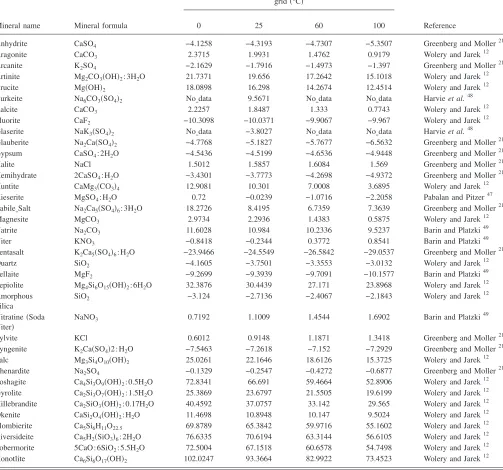
The comparison of experimental results and model pre-dictions of the evaporation of synthetic Topopah Spring Tuff pore water at 95 ° C indicates that the current high-temperature Pitzer database used by the Yucca Mountain pro-gram adequately describes the chemical evolution of brines at elevated temperature for most species共Fig. 3兲. In this sec-tion we discuss our results in light of the high temperature Pitzer ion interaction database that includes solubility prod-ucts for solids. Table II lists temperature-dependent Pitzer
interaction parameters for binary and ternary reactions and Table V details the solubility products relevant to this work. The Yucca Mountain Project high temperature Pitzer ion interaction database is the most comprehensive database available to account for the nonideal behavior of highly con-centrated electrolytes over a wide range of temperature
共0 – 140 ° C兲. The database was founded on the original variable-temperature Pitzer parameters20,21supplemented by parameter data from several other sources.13,22–32 It also in-cludes thermodynamic parameters converted from non-standard Pitzer equations from the published literature.14 Temperature-independent parameters based on 25 ° C data are used for several parameters where temperature dependent data are lacking.13 The database contains temperature-dependent ion interaction parameters for most ion groups relevant to our experimental system at 95 ° C. Exceptions include 25 ° C models for potassium nitrate interactions and some calcium and magnesium ion interactions;13 and 20– 90 ° C models for CO2共aq兲ion interactions.26Substantial
database and model validation has been performed,1 how-ever, it is acknowledged that the results of any model are only as good as the input parameters and database used, and typically, improvements will always be made to bridge the gaps between experimental observations and model predic-tions.
1. Na+, Cl−, K+, and NO 3 −
The excellent agreement between model prediction and experiment for sodium, chloride, potassium, and nitrate sug-gests that the high temperature Pitzer ion interaction data-base and halite solubility product adequately describes the nonideal solution chemistry at high ionic strength and el-evated temperature for these elements, as well as the halite solubility product. The agreement is expected for sodium and chloride because interaction parameters for binary and ter-nary ion groups are well defined as a function of temperature.14,21,25,27,33–35
The excellent agreement between prediction and experi-ment for potassium and nitrate suggests that Pitzer param-eters for the K+– NO
3
−ion interaction will yield accurate
pre-dictions of pore water concentrations in evaporating solutions despite being measured at 25 ° C and applied to 95 ° C systems. The reason for this is that high sodium to potassium, and chloride to nitrate mole ratios seen in our experiments may effectively mask any mismatch due to con-stant 25 ° C parameters. Clearly, this is true for undersatu-rated brines with respect to KNO3共niter兲because Na+– NO3−
and K+– Cl− interactions will be more important than
K+– NO 3
− interactions in determining solution properties.
However, when brines are saturated with niter共KNO3兲, then
K+– NO 3
−interactions are more important. The extent that the
constant temperature K+– NO 3
− interaction parameter does
not accurately predict behavior was shown in KNO3– NaNO3 deliquescence experiments at 90 ° C. In