PREDICTING HEART DISEASES IN LOGISTIC REGRESSION OF MACHINE LEARNING ALGORITHMS BY PYTHON JUPYTERLAB

Predicting Heart Diseases In Logistic Regression Of

Machine Learning Algorithms By Python Jupyterlab

A. S. Thanuja Nishadi

University of Colombo, Faculty of Graduate Studies, Sri Lanka, [email protected]

Abstract: Healthcare expenditures are overwhelming national and corporate budgets due to asymptomatic diseases including cardiovascular diseases. Therefore, there is an urgent need for early detection and treatment of such diseases. Machine learning is one of the trending technologies which used in many spheres around the world including healthcare industry for predicting diseases. The aim of this study is to identify the most significant predicators of heart diseases and predicting the overall risks by using logistic regression. Thus, binary logistic model which is one of the classification algorithms in machine learning is used in this study to identify thepredicators. Further, data analysis is carried out in Python using JupyterLab in order to validate the logistic regression.

Keywords: machine learning, logistic regression, classification algorithms, heart diseases

1.

Introduction

The number of deaths due to cardiovascular diseases increased by 41% between 1990 and 2013, climbing from 12.3 million deaths to 17.3 million deaths in globally. In addition to that, half of the deaths in the United States and other developed countries are due to the same issue [1].Therefore, early detection of heart diseases is required to reduce the health complications. Machine learning has been widely used in modern healthcare sector for diagnosing and predicting the presence of diseases using data models. Logistic regression is one such relatively used machine learning algorithms for studies involving risk assessment of complex diseases. Thus, the study intends to identify the most significant predicators of cardiovascular diseases and predicting the overall risk by using logistic regression.

2.

Background of the study

The dataset which used for the logistic regression analysis is available on the Kaggle website(https://www.kaggle.com), from an ongoing cardiovascular study of Framingham, Massachusetts. The classification goal of this study is to predict whether the patient has 10-year risk of future heart diseases. The Framingham dataset consists with 4238 records ofpatients’dataand15attributes.Thedataanalysisiscarried out in Python programming by using JupyterLab which is more flexible and powerful data science applicationsoftware.

3.

Machine Learning (ML)

Machine learning is widely used in almost many fields in the world including healthcare sector. Machine learning is an application of artificial intelligence (AI) that provides systems the ability to automatically learn and improve from experience without being explicitly programmed [2]. Further, machine learning at its most basic is the practice of using algorithms to parse data, learn from it, and then make a determination or prediction about something in the world [3]. There are two major categories of problems often solved by machine learning i.e. regression and classification. Mainly, the regression algorithms are used for numeric data and classification problems include binary and multi-category problems [4].Machine learning algorithms are

further divided into two categories such as supervised learning and unsupervised learning [5]. Basically, supervised learning is performed by using prior knowledge in output values whereas unsupervised learning does not predefined labels hence the goal of this is to infer the natural structures within the dataset [6]. Therefore, selection of machine learning algorithm need to carefully evaluated.

4.

Logistic Regression Model

Logistic regression is a one of the machine learning classification algorithm for analyzing a dataset in which there are one or more independent variables (IVs) that determine an outcome and also categorical dependent variable (DV)[7]. Linear regression uses output in continuous numeric whereas logistic regression transforms its output using the logistic sigmoid function to return a probability value which can then be mapped to two or more discrete classes [8]. The logistics regression forms three types as below.

a) Binary logistics regression (two possible outcomes in a DV)

b) Multinomial logistics regression (three or more categories in DV without ordering)

c) Ordinal logistics regression (three or more categories in DV with ordering) [9]

Furthermore, logistic regression model uses more

complex costfunction

(knownassigmoidfunctionorlogisticfunction) instead of linear function[10]. Logistic regression limits the cost function between 0 and1.

Figure 1: Logistic Regression

According to the given data set, 1 indicates the high risk of 10-year future coronary heart disease and 0 indicates non or no heart risks. The independent variables n in the logistic model as x1, x2, x3……., xn

(

)

Logisticregressionachievesthisbytakingthelogoddsofthe event ln(P/1−P), where, P is the probability of event which is risk of CHD. Therefore, P always lies between 0 and1.

5.

Methodology

5.1 Workflow of Machine Learning ModelBuilding

Figure 2 indicates the steps followed in order to build the logistic regression model in machine learning.

Figure 2: Workflow of Logistic Regression Model

5.1.1Data Acquisition

The dataset is collected from Kaggle website.

5.1.2Data Pre-Processing

In order to build up more accurate ML model, data pre- processing is required. Data pre-process is the process of cleaning the data. This includes identification of missing data, noisy data and inconsistent data.

5.1.3Select Machine LearningModel

The pre-processed data are identified using machine learning algorithms.

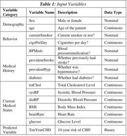
a) Input Variables of the study

The data set consists with 14 IVS and predicted value. ML model is based on identification of DV. It has used binary logistic regression which is one of the classification algorithms due to target variable is categorical.

Table 1: Input Variables

Variable

Category Variable Name Description Data Type

Demographic Sex Male or female Nominal age Age of the patient Continuous

Behavior currentSmoker Current smoker or not? Nominal cigsPerDay Cigarettes per day? Continuous

Medical History

BPMeds Blood

pressuremedication? Nominal

prevalentStroke Whether previously had

stroke? Nominal

prevalentHyp Whether was

hypertensive? Nominal

diabetes Whether had diabetes? Nominal

Current Medical Status

totChol Total Cholesterol Level Continuous

sysBP Systolic Blood Pressure Continuous

diaBP Diastolic Blood Pressure Continuous

BMI Body Mass Index Continuous

heartRate Heart Rate Continuous

glucose Glucose Level Continuous Predicted

Variable TenYearCHD 10-year risk of CHD Binary

6.

Data Analysis

Data Analysis was carried out using Jupyter Lab using Python. The following steps were implemented in order to process the logistics regression.

6.1 Loading Data and Other Required Libraries

It has loaded the heart prediction data using Framingham CSV file into Jupiter Lab in Order to build the logistic regression model. In addition to that, required libraries which used as supportive applications are loaded. It has removed the education field from the database.

6.2 Exploratory Data Analysis(EDA):

6.3 Identify Missing Values

Further, the number of missing values has identified for cleaning existing dataset. The summarized total number of missing values based on the attributes are given below.

Then, the total percentage of missing values in column was identified using Pandas Data Frame. Total number of rows with missing values is 489 since it is only 12 percent of the entire dataset the rows with missing values are excluded. It has used Pandas dropna() method which was used to analyze the drop rows/columns with Null values.

The descriptive figures related to 10year risk of CHD has indicated below.

According to the above data, there are 3179 patents with no heart disease and 572 patients with risk of heart disease.

6.4 Implementing Logistic Regression

The following outcomes are used to indicate the logistic regression. Logistic regression is mainly used to for prediction and also calculating the probability of success.

The above output indicates the result after using backward elimination. The logistic regression equation for the heart prediction data as follows.

( ) ( )

6.5 Interpreting Logistic Results

The following methods indicates the accuracy measurements.

a) Interpreting Odds Ratio(OR):

This is used to measure the association between an exposure with outcome. Further, the odds ratio can also be used to determine whether a particular exposure is a risk factor for a particular outcome, and to compare the magnitude of various risk factors for that outcome.

 OR=1 Exposure does not affect odds of outcome

 OR>1 Exposure associated with higher odds of outcome

 OR<1 Exposure associated with lower odds of outcome

b) Confidence Intervals(CI):

The accuracy of OR is estimated by using 95% confidence interval (CI). A large CI represents the low level of precision of OR and also small CI represents the higher precision of OR. However, 95% CI does not indicate the statistical significance unlike the p value.

 According to the fitted model, the odds of diagnosed with heart disease of males (78.8%) is higher than the females.

 Further, the odds of diagnosis with CHD is increase approximately 7% for a one-year age increase (1.067571)

 In addition to that, additional cigarette has risk of 2% increase in odds of CHD.

 Furthermore, odds of sysBP has 1.7% increase in every unit increase.

 No significance changes in the total cholesterol level and glucose level.

6.6 Training and testing sets

Data set was separated into training and testing sets for evaluation process. This has been done using scikit-learn library.

The accuracy of the model is 0.87.

6.7 Confusion Matrix Outcomes

This has used to indicate the summary of prediction results including correct and incorrect on a classification problem. Further, this was used to not only errors but also types of errors. The segments of the confusion matrix indicate the following parameters.

 True Positives (TP): cases which are predicted yes (they have the disease), and they do have the disease.

 True Negatives (TN): cases which are predicted no, and they do not have the disease.

 False Positives (FP): cases which are predicted yes, but they do not actually have the disease (Type I error).

 False Negatives (FN): cases which are predicted no, but they actually do have the disease (Type II error).

Correct predictions (646+4) =650 Incorrect predictions (99+1) =100

Therefore, True Positives:4 True Negatives:646

False Positives:1(Type I error) False Negatives:99(Type II error)

This is a list of rates that are often computed from a confusion matrix for a binary classifier:

It has been checked the accuracy of the model using confusion matrix.

Terms Formula

Accuracy of the model (overall, how often the classifer correct)

(TP+TN)/(TP+TN+FP+FN)

Misclassification Rate (overall, how often it wrong or error rate)

(FP+FN)/(TP+TN+FP+FN)

Sensitivity or True Positive Rate

(when it is actually yes, how often does it predict yes)

TP/(TP+FN)

Specificity or True Negative Rate

(when it is actually no, how often does it predict no)

TN/(TN+FP)

With analyzing confusion matrix data, it is evident that the model is highly specific than sensitive. Further, the negative values in the model are predicted more accurately than the positives.

6.8 ROC Curve

The ROC Curve is a simple plot which used to visualize the performance of a binary classifier. Further, this shows the tradeoff between the true positive rate and the false positive rate of a classifier for various choices of the probability threshold.

Good classification accuracy models should have significantly more true positives than the false positives at all thresholds. Area Under the Curve(AUC) quantifies the model classification accuracy.

7.

Conclusion

References

[1]. Mozaffarian, D., Benjamin, E., Go, A., Arnett, D., Blaha, M.Cushman, M. et al. (2015). Heart Disease

and Stroke Statistics—2015,

Update. Circulation, 131(4). doi:

10.1161/cir.0000000000000152.

[2]. Das, S., Dey, A., Pal, A., & Roy, N. (2015). Applications of Artificial Intelligence in Machine Learning: Review and Prospect. International Journal of Computer Applications, 115(9), 31-41. doi: 10.5120/20182-2402

[3]. Abduljabbar, R., Dia, H., Liyanage, S., & Bagloee, S. (2019). Applications of Artificial Intelligence in Transport: An Overview. Sustainability, 11(1), 189. doi: 10.3390/su11010189

[4]. Strecht, Pedro & Cruz, Luís & Soares, Carlos & Moreira, João & Abreu, Rui. (2015). A Comparative Study of Classification and Regression Algorithms for Modelling Students' Academic

Performance, ,

https://www.researchgate.net/publication/27803068 9_A_Comparative_Study_of_Classification_and_R egression_Algorithms_for_Modelling_Students'_Ac ademic_Performance, viewed: 10th June 2019.

[5]. Sathya, R & Abraham, A (2013) International Journal of Advanced Research in Artificial Intelligence, Vol. 2, No. 2, 2013, http://ijarai.thesai.org/Downloads/IJARAI/Volume2

No2/Paper_6-Comparison_of_Supervised_and_Unsupervised_Le arning_Algorithms_for_Pattern_Classification.pdf, viewed: 10th June 2019.

[6]. CVA, K. (2017),

https://www.medwinpublishers.com/JOBD/JOBD1 6000139.pdf. Journal of Orthopedics & Bone Disorders, 1(7). doi: 10.23880/jobd-16000139

[7]. Miguel-Hurtado, O., Guest, R., Stevenage, S., Neil, G., & Black, S. (2016). Comparing Machine Learning Classifiers and Linear/Logistic Regression to Explore the Relationship between Hand

Dimensions and Demographic

Characteristics. PLOS ONE, 11(11), e0165521. doi: 10.1371/journal.pone.0165521

[8]. Ng, A. Y. and Jordan, M. I. (2002). On discriminative vs. generative classifiers: A comparison of logistic regression and naive bayes. In NIPS 14, pp. 841–848.

[9]. Peng, C., Lee, K., & Ingersoll, G. (2002). An Introduction to Logistic Regression Analysis and Reporting. The Journal of Educational

Research, 96(1), 3-14. doi:

10.1080/00220670209598786

[10]. Park, H. (2019). An Introduction to Logistic Regression: From Basic Concepts to Interpretation