IMAGE DENOISING USING SPATIAL DOMAIN FILTERS

42 | P a g e

IMAGE DENOISING USING SPATIAL DOMAIN

FILTERS

Iffat Rehman Ansari

University Women’s Polytechnic, Aligarh Muslim University, Aligarh 202002, U.P., India

ABSTRACT

In image processing, the first pre-processing step is to denoise an image and it is supposed to be one of the most

important tasks. In order to perform image denoising, an image is processed in such a way that various

restoration techniques are used to remove induced noise as image may be corrupted with noise during

acquisition, transmission or, compression process. Noise is a very common problem in images due to which the

visual quality of an image is degraded and it may be Additive white gaussian noise, Impulsive noise and

Multiplicative noise etc. The main aim of restoration techniques is to produce an image that closely resembles

to the original image. In this research work, noisy images are generated by introducing various types of noise

models in the original noise-free image and image denoising is performed by applying various types of spatial

filters to different noise models. As far as the quality of an image is concerned here, it is examined by objective

evaluation of an image. In this paper, one of the most important metrics called peak signal to noise ratio (PSNR

in dB) is used which shows the filtering performance of a particular spatial domain filter and it also gives

quantitative information of the noisy and denoised image.

Keywords:

Noisy Image, Denoised/Filtered Image, Peak Signal to Noise Ratio (PSNR).

I. INTRODUCTION

Image Denoising/ Noise Reduction is one of the traditional crisis in image processing [1]. As far as image

denoising is concerned, it has remained a major problem in the field of image processing [2]. Often, images are

corrupted by noise due to some imperfections in image acquisition systems &transmission channels that results

in image degradation which in turn causes a significant reduction of image quality and this makes high-level

vision tasks like recognition, 3D reconstruction, or scene interpretation much more difficult. There are several

reasons that may cause an image degradation such as blur, motion and noise [3] but denoising has been always a

major concern in image processing since decades [4]. Thus image denoising is itself an important image

processing task as well as an important pre-processing step in image processing pipeline[5].The operation which

is performed on an image affected by unwanted noise is referred to as an image denoising as unwanted noise

adds spurious and extraneous information to an original image. This kind of unwanted noise leads to destruction

of minute details in the image and such a noisy image is undesirable for human perception and for machine tasks

too. Image denoising is performed to reduce or remove the noise while retaining most of the important signal

features as it is [6].

The technique in which a noise free image is recovered from a corrupted and degraded image is referred to as an

43 | P a g e

degradations and then an inverse procedure is applied to get an approximation of the original image [7].

Generally, denoising and de-blurring tasks come under this category. Thus image denoising is one of the most

effective and efficient restoration process [8].

Digital filters are used to remove noise from the degraded image as any noise in the image can cause serious

errors [9]. Thus the filters are the inverse degradation models of the image and when they are applied to a

corrupted or degraded image, an original image can be reconstructed. As far as an image is concerned, edges

and fine details are actually the high frequency contents and carry very important information. So, those filters

are highly suitable for digital image filtering which can efficiently preserve edge and image detail [10]. The

filters can be broadly classified into two major types i.e. Spatial Domain Filters and Transform Domain Filters.

Such filters are designed in such a way that they can be used for one specific type of degradation & noise model

and some filters can be useful for other types as well but no image restoration technique is universal that is

suitable for all types of noise models [11]. In order to remove the noise, the noisy signal has to be passed

through a filter which in turn removes the undesirable components while retaining the desirable one and the

filters used for image denoising may be linear or non-linear depending on the type of noise [12].

In this paper, various spatial domain filters used for the removal of noise are discussed. These filters are applied

on different noisy images having different types of noise models induced, their performance is evaluated in

terms of PSNR and noisy & denoised signals are compared on the basis of PSNR.

II. NOISE MODELS

It is to be noted that the noise is undesired information which contaminates the original image. There are various

types of noise that corrupts an image and the noise may be present in an image either in an additive form or in

multiplicative form [7] but for an efficient denoising technique, information about the type of noise present in

the degraded image is very important. A model comprises of image degradation process as well as image

restoration process is shown in figure (1).

Here, the degradation function and inverse degradation function can be mathematically represented by following

equations:

g(x, y) = f(x, y) ∗ h(x, y) + n(x, y) (1)

f̂(x, y) = D . g(x, y) (2)

where, f(x,y) is the original noise free image, h(x,y) be the degradation function, n(x,y) is the additive noise

44 | P a g e

restoration model. The various types of noise models are discussed below:

2.1 GAUSSIAN NOISE

It is one of the most commonly found noise in images and also called Additive White Gaussian Noise (AWGN)

or normal noise. This type of noise is generally added to an image during image acquisition like sensor noise

which is caused by low light, high temperature and transmission such as electronic circuit noise or Amplifier

noise [14].The Probability Density Function (PDF) of Gaussian distribution [15] is given by equation (3) and its

plot is shown in figure (2).

P(z) = 1

√2πσe −(z−μ)2

2σ2 (3)

where, z represents the gray level, µ is the mean or average value of z, σ be the standard deviation of the noise

and σ2 _{is the variance of z.}

2.2 SALT & PEPPER NOISE

Another kind of noise that is present during the image transmission is Salt &Pepper noise [16]. Salt and pepper

noise is also called an Impulse noise or Spike noise. It appears as white and/or black impulse of the image and

caused due to malfunctioning of pixels in camera sensors, faulty memory locations in hardware, or transmission

in a noisy channel [17]. Due to this type of noise, white and black spots are appeared in gray scale images. In

other words, salt &pepper noise results in dark pixels in bright regions and bright pixels in dark regions in an

image [18].The PDF of Impulse noise is given by equation (4) and it is represented graphically as shown in

figure (3).

P(z) = {ppba, for z = a, for z = b

0, otherwise

(4)

2.3 POISSON NOISE

The Poisson noise is a type of electronic noise and it is also referred to as Photon noise or Shot noise. If number

of photons sensed by the sensor is not sufficient enough to provide detectable statistical information, then such

type of noise occurs having Poisson distribution [19]. The PDF of Poisson Noise [13] is given by equation (5)

and its plot is shown in figure (4).

P(z) = (e−λ λz

z!) , for z = 0,1,2, … … … .. (5)

45 | P a g e

The Uniform noise arises due to quantization of pixels of an image to a number of discrete levels. Hence it is

also known as Quantization noise and has approximately uniform distribution. Thus various levels of gray

values of the noise are uniformly distributed over a specified range and this type of noise provides one of the

most neutral noise. The PDF of Uniform noise [13] is given by equation (6) and its plot is shown in figure (5).

P(z) = {

1

(𝑏−𝑎), for a ≤ z ≤ b

0, otherwise (6)

The mean and variance of Uniform noise are defined as:

μ =(a+b)₂ and 𝜎2₌(𝑏−𝑎)2 12

2.5 RAYLEIGH NOISE

This type of noise can be modeled by the Rayleigh distribution and is typically found in RADAR range and

velocity images. The PDF of Rayleigh noise is given by equation (7) and it is represented graphically as shown

in figure (6).

P(z)={2b(z − a)e

−(z−a)2

b , for z ≥ a

0, 𝑓𝑜𝑟 𝑧 < 𝑎 (7)

The mean and variance of Rayleigh noise are given as:

μ = 𝑎 + √𝜋𝑏₄ and 𝜎2₌𝑏(4−𝜋) 4

2.6 GAMMA NOISE

The Gamma noise is also known as Erlang noise. The PDF of Gamma noise is given by equation (8) and its plot

is shown in figure (7).

P(z)={

ab_z(b−1)

(b−1)! e−az, for z ≥ 0

0, 𝑓𝑜𝑟 𝑧 < 0 (8)

46 | P a g e

μ =b_a and 𝜎2= b

a2

2.7 EXPONENTIAL NOISE

This type of noise is a special kind of Gamma noise having value of positive integer b equal to unity. The PDF

for Exponential noise is given by equation (9) and it is represented graphically as shown in figure (8).

P(z)={_{0, 𝑓𝑜𝑟 𝑧 < 0}𝑎𝑒−𝑎𝑧, for z ≥ 0 (9)

The mean and variance of Exponential noise can be defined as:

μ =1_a and 𝜎2= 1

𝑎2

2.8 SPECKLE NOISE

The Speckle noise is a granular noise, multiplicative in nature and severely corrupts an image [20]. When the

magnitude of image pixel is high then the noise will also be high. Thus, this type of noise is a signal dependent

noise and it is also known as multiplicative noise. As far as speckle noise is concerned, it is usually encountered

in almost all coherent imaging systems like laser, acoustics, SAR (Synthetic Aperture Radar), bio-medical

applications like ultrasonic imaging. Such type of noise reduces the image resolution and contrast due to which

the diagnostic value of this imaging modality is affected. Hence, reduction of speckle noise is an essential

pre-processing step especially in the case of ultrasound imaging used for medical imaging. This particular noise

47 | P a g e

III. IMAGE DENOISING FILTERS IN SPATIAL DOMAIN

By using various filters, the noise in the noisy image can be filtered out while retaining the desirable

components. Thus filter is supposed to be one of the most important subsystem of any signal processing

systems. In the spatial domain, filters are broadly classified into two major categories i.e. linear filters and

non-linear filters. In non-linear filtering, lines &other fine details present in the image are destroyed and sharp edges are

generally blurred. In order to preserve signal structure especially edge information, non-linear filtering

techniques are used and become more popular. The median filter first suggested by Tukey in 1971 is the most

popular order statistics filter among non-linear image filters [10]. Actually, the type and amount of noise present

in an image decides the type of filter to be used for denoising a particular noisy image because various filters are

capable of removing various types of noise efficiently and some of the filters under spatial domain category are

discussed below:

3.1 ARITHMETIC MEAN FILTER

The filtering operation which is performed directly on the image pixels is referred to as Spatial Filtering and in

this filtering process, the filter mask is simply moved from one point to another point in an image. The

arithmetic mean filter is supposed to be one of the most simplest linear filter among the existing spatial filters

and it is also known as the averaging filter because its output is actually the average of all pixels lying in the

neighbourhood of the filter mask. In other words, it simply determines the average value of all intensities of the

neighbourhood of the centre pixel in an input image and this particular centre pixel is replaced by the average

value in the output image. This filter is also called a smoothing filter because it decreases the variations of

intensity between adjacent pixels [11] but it blurs the edges of the image and is commonly useful in removing

irrelevant details from an image [13]. Mathematically, the mean filter can be represented by equation (10):

f̂(x, y) =_(mn)1 ∑{g(s, t)} where, (s, t) ∈ sxy (10)

Here, the filter operates on (m x n) mask, Sxy represents the set of coordinates in a rectangular subimage window having a center at (x,y). This particular filter calculates the mean or, average of the corrupted image g(x,y) under

the area Sxy, and f̂(x,y) represents the reconstructed or, restored image. Generally, linear filters are used for noise suppression [19].

3.2 MEDIAN FILTER

The median filter is one of the most popular order statistic or, rank filter due to its edge preserving nature [21]. It

is most commonly used non-linear filter and non-linear filter can be effectively used in noise reduction. In this

particular filter, the pixel value of image is actually replaced by the median value. The median filter is excellent

at noise removal and can be mathematically represented by equation (11):

f̂(x, y) = median {g(s, t)} where, (s, t) ∈ sxy (11)

3.3 MINIMUM (MIN) FILTER

The minimum filter is also referred to as the 0th _{percentile filter. This type of filter replaces the value of the pixel} with the minimum intensity level of the neighbourhood of that pixel and it actually finds the darkest points in an

48 | P a g e

f̂(x, y) = min {g(s, t)} where, (s, t) ∈ sxy (12)

IV. RESULTS & DISCUSSION

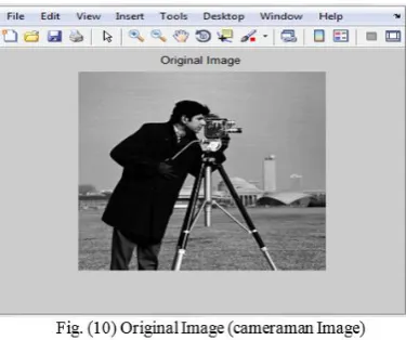
To perform the simulation, matlab software is used. Here, the original image shown in figure (10) is a standard

grayscale cameraman image of size256 x 256.

The main aim is to introduce different types of noises in an original image and filtering out them using various

types of filters. The results obtained are discussed and shown in figures (11) to (18).

 Firstly, noisy image shown in figure (11a) is created by adding gaussian noise to an original image which is

then filtered out by median filter. Now, the filtered image shown in figure (11b) is produced which resembles

to an original image. It shows that the median filter is the best to discard gaussian noise.

 Again, noisy image shown in figure (12a) is generated by introducing salt & pepper noise in an original image

and this type of noise is well filtered out by using median filter that gives us a filtered image as shown in

figure (12b). With this filter, the salt & pepper noise is almost completely filtered out and the final image

looks like the original one. As far as the quality and clarity of filtered image is concerned, median filter gives

49 | P a g e

then this noise is filtered out by using median filter. Hence, filtered image shown in figure (13b) is created but

the final image shows that this filter does not completely remove the noise.

 Now, the noisy image shown in figure (14a) is created by adding uniform noise to an original image. This

type of noise is filtered out by using min filter and the filtered image shown in figure (14b) looks like an

original image but not exactly same. It means that this type of filter does not remove the noise completely but

partially.

 Another noise that is added to an original image is of rayleigh type and the noisy image is shown in figure

(15a). To filter out this noise from the noisy image, min filter is used and the filtered image shown in figure

(15b) is generated but the quality of the final image is not good.

 Now, the noisy image shown in figure (16a) is generated by adding exponential noise to an original one and

noise filtering is accomplished by using arithmetic mean filter. This filter removes the noise to a certain extent

50 | P a g e

shown in figure (17a). To remove this noise, median filter is used and the filtered image shown in figure (17b)

is obtained which closely resembles to that of the original image. It means that the median filter is best fit for

the gamma noise.

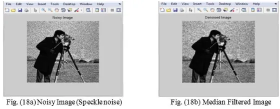
 Finally, the noise that corrupts an original image is the speckle noise and the noisy image is shown in figure

(18a). In order to discard this type of noise, median filter is used. It gives best result in terms of clarity of an

image that can be depicted from figure (18b).

In this research work, the quantitative performance of the spatial filters is accessed by one of the most important

quality metrics i.e., peak signal to noise ratio (PSNR) measured in decibel (dB) and for gray scale, it can be

mathematically represented by equation (13):

PSNR = 10 log10(255

2

MSE) (13)

where, MSE is the mean square error between the original and the denoised image.

Table (1) depicts the filtering performance of various spatial domain filters in terms of PSNR operated on

51 | P a g e

PSNR for various noise models.

The more the value of PSNR of denoised signal with respect to the PSNR of noisy signal, the better is the

quality of the filtered/denoised image.

V. CONCLUSION

In this research work, the concept of image degradation and restoration has been discussed. Here, the eight

different types of noise models including gaussian, salt & pepper, poisson, uniform, rayleigh, exponential,

gamma and speckle noise have been discussed and simulated on the standard cameraman image. The linear and

non-linear spatial domain filtering techniques also have been discussed. Then different spatial filters including

arithmetic mean, median and min filter have been discussed and applied on various noisy images to filter out the

noise. The performance of various filters has been evaluated on the basis of PSNR. According to the simulation

results, the best filter is the median filter to remove gaussian, salt & pepper, poisson, gamma and speckle noise

respectively while min filter removes uniform & rayleigh noise efficiently and arithmetic mean filter performs

well in removing exponential noise. On the other hand, there are certain limitations of image filtering in spatial

domain as it does not remove the noise from the degraded image completely rather partially and increase in the

density of noise in an image would result in the blurred image after filtering which is undesirable. But

irrespective of these limitations, most of the spatial filters reconstructs the original image from the degraded

52 | P a g e

REFERENCES

[1] Rangaraj M. Rangayyan, “Biomedical Signal Analysis: A Case study Approach”, IEEE Press, 2005

[2] M. C. Motwani, M. C. Gadiya, R. C. Motwani, Jr. F. C. Harris, “Survey of image denoising techniques”,

Proceedings of Global Signal Processing Expo and Conference, Santa Clara, CA, USA, September 2004

[3]Charu Khare and Kapil Kumar Nagwanshi, “Image Restoration Technique with Non Linear Filter”,

International Journal ofAdvanced Science and Technology, Vol. 39, pp. 67-44, February 2012

[4] H. J. Seo, et al, “A comparison of some state of the art image denoising methods", Conference Record of the

Forty-First Asilomar Conference on Signals, Systems and Computers, 2007, pp. 518 – 522, ACSSC, 2007

[5] Xiang-Yang Wang, Hong-Ying Yang, Zhong-Kai Fu, “A New Wavelet-based image denoising using

undecimated discrete wavelet transform and least squares support vector machine”, Expert Systems with

Applications (37)- Elsevier, pp. 7040–7049, 2010

[6] S. Gupta, L. Kaur, R. C. Chauhan and S. C. Saxena, “A Versatile technique for visual enhancement of medical ultrasound images”, Digital Signal Processing, Vol. 17, No. 3, pp. 542-560, May 2007

[7] A. K. Kanithi, “Study of Spatial and Transform Domain Filters for Efficient Noise Reduction”,Master Of

Technology Thesis submitted to National Institute of Technology, Rourkela in 2011

[8]Kalavathy. K, “Image Denoising using Filtering andThreshold techniques in WaveletDomain”, Doctor of

Philosophy Thesis submitted to Educational and Research Institute, Dr. M.G.R University, Chennai inJuly 2012

[9]A.K.Jain, "Fundamentals of Digital Image Processing", Engelwood Cliff, N. J., Prentice Hall, 2006

[10]T. K. Thivakaran and Dr. RM. Chandrasekaran, “Nonlinear Filter Based Image Denoising Using AMF

Approach”, International Journal of Computer Science and Information Security(IJCSIS), ISSN: 1947-5500,

Vol. 7, No. 2, 2010

[11] Jappreet Kaur, et al, “Comparative Analysis of Image Denoising Techniques”, International Journal of

Emerging Technology and Advanced Engineering, Vol. 2, June 2012

[12] T.S. Huang, G.J. Yang, and G.Y. Tang, "A Fast Two Dimensional Median Filtering Algorithm", IEEE

Transaction on Acoustics Speech, Signal Processing, Vol. ASSP-27, No.1, Feb 1997

[13] R. C. Gonzalez and R. E. Woods, “Digital Image Processing”, Pearson Education India, 2009

[14] J. H. Wang, W. J. Liu, and L. D. Lin, “Histogram-based fuzzy filter for image restoration,” IEEE Trans.

Syst. Man Cybern. B, bern, vol. 32, no. 2, pp. 230–238, Apr. 2002

[15] A. Aboshosha, et al, "Image denoising based on spatial filters, an analytical study", International

Conference on Computer Engineering & Systems, 2009, ICCES 2009, pp. 245-250, IEEE 2009

[16] J.S.Lee,"Digital Image Enhancement and Noise Filtering by use of Local Statistics", IEEE Trans. On

Pattern Analysis and Machine Intelligence, Vol. PAMI-29, March, 1980

[17] A. Bovik, “Handbook of Image and Video Processing”, New York: Academic, 2000

[18]Charles Boncelet & Alan C. Bovik, “Image Noise Models”, Handbook of Image and Video Processing,

53 | P a g e

of Computer Applications (0975 – 8887), Volume 9– No.4, November 2010

[20] Guo H., Odegard J. E., Lang M., Gopinath R. A., Selesnick I. W and Burrus C. S., “Wavelet based speckle

reduction with application to SAR based ATD/R”, First International Conference on Image Processing, Vol. 1,

1994

[21] Raymond H. Chan, Chung-Wa Ho, and Mila Nikolova, “Salt&Pepper Noise Removal by Median Type

Noise Detectors & Detail Preserving Regularization”, IEEE Trans. on Image Processing, Vol. 14, No.