© Global Society of Scientific Research and Researchers http://ijcjournal.org/
Comparative Study of Image Denoise Algorithms
Tram Tran Nguyen Quynh
a, Hung Do Phi
b*a,bFaculty of Information Department, Ho Chi Minh City University of Foreign Languages and Information
Technology 155 Su Van Hanh (extent), District 10, Ho Chi Minh City, 700000, Vietnam
aEmail: [email protected]
bEmail: [email protected]
Abstract
Denoising is a pre-processing step in digital image processing system. It is also typical image processing challenges. Many works proposed to solve problem with new approaching. They can be divided into two main categories: spatial-based or transform-based. Some denoising methods apply in both spatial and transform domains. The goal of this paper focuses on reviewing denoise methods, classifying them into different categories, and identifying new trends. Moreover, we do experiments to compare pros, cons of methods in survey.
Keywords: Denoise; Bilateral Filter; Guided Image Filter; ROF; TV-L1; Total Variation; Wavelet shrinkage; Dual-domain image denoise; Non-local dual denoising.
1.Introduction
Digital image can degraded by noise in the process of capture, acquisition, processing and transmission. Therefore, image denoising is one of the challenges in image processing and computer vision with removing the noise from given noisy image in data acquisition to predict original image. A good image denoising model is eliminating noise as much as possible while preserving the characteristics of the image such as edges, corners and other sharp structures, etc. [1]. Two main approach to image denoising is based on spatial domain, and transform domain. Besides, there are some image denoising methods applied in both spatial and transform domain. Approaching denoise in spatial domain, Tomasi and his colleagues [2] proposed a smoothing filter with properties edge preserving and noise-removing for images called Bilateral Filter. Bilateral filter [3] solves the limitation of Gaussian filter [4] by the difference in values with the neighborhood to preserve edges. In bilateral filter, the influence of a pixel to another one should not only occupy a nearby location but also have a similar value.
Though bilateral may not be the best noise reducing filter but it is good and simple. Also, it can be used for tone mapping, relighting and texture editing. However, the nonlinear operator is hard to compute since it is complex and spatially varying kernels. Besides, it causes staircase effect, gradient reversal, and artifact near edges. All the shortcomings are covered with the improved with Guided image filter.
Guided image filter [5] is an edge preserving smoothing filter which output is locally a linear transform of the guidance image. It has good edge-preserving smoothing properties like bilateral filter but it solves the unwanted problems which occurs in bilateral filter. Guided filter has a O(N) time non-approximate algorithm, independent of the window radius and the intensity range. Also, it is easily implement and avoid staircase effect and artifacts. It is good to be applied in feathering, matting, single image haze removal and joint up sampling. However, despite its advantage, guided filter also has its own limitation which is the exhibit halos near some edges when the image is being smoothing which is shown in Figure5. Besides, it does not effectively reduce noise because its output values are unchanged within high-variance region.
Among methods in denoise using spatial domain, non-linear variational methods such ROF and TV-L1 total variational method [6, 7] were one of effective method to reduce noise but also keep edge-preserving. It bases on principle that signal detail is dense and smooth in variability. To obtain denoise image, it is an ill-pose problem with many solutions. So, the best solution is image with slowest variation or smoothness. All of properties above result to minimization problem with solving energy function with data term for assuming noise distribution with mean 0 and smoothness term about softness variability in details.
Approaching transform domain, image will transform into frequency domain to eliminate noise signals corresponding to "small" coefficients. Hard and soft thresholding will remove these values when they are less than specific thresholding. Wavelet shrinkage method [8] bases on thresholding of small wavelet coefficients. By eliminating theses values, the noise will be removed out of data. It takes pros than spatial domain method when keeping low contrast details. However, it produces many artifacts.
The current state-of-the-art denoise methods is approach on taking advantages of spatial and transform domain. On spatial domain, these methods discover self-similarity in the image itself. In other words, they model patch space of an image and denoise by normalization similar patches. Besides, it will reduces noise signal in the patches by transforming frequency domain and thresholding small coefficients.
Dual-domain image denoise [9] is unmistakably simple method in implementing. Besides, it also has good results in PSNR comparing with different methods in same approach [10, 11]. However, because of using noise image for guided image, it also procedures artifacts as common errors of transform domain methods. Non-local dual denoising [12] is a faster and better method more than Non-local dual denoising method. It avoids artifacts by applying NL-Bayes for building guided image. And it only uses one step to remove noise on spatial and frequency domain.
Next, in transform domain, we also introduce about wavalet shrinkage denoise. Last, we will study methods approaching spatial and transform domain for denoise such dual domain image denoise, Non-Local dual denoise.
The organization of this paper is as follows. In Section II, III, IV, we introduce about image denoising and a synthesis of image filtering methods. Experiments results are discussed in Section V, followed by the conclusion and future work in the Section VI.
2.Spatial Domain methods
2.1.Bilateral Filter
In 1998, Carlo Tomasi and Roberto Manduchiis [2] proposed a new a nonlinear, edge preserving and noise-reducing smoothing filter for images called Bilateral Filter. Bilateral filter [3] solves the limitation of Gaussian filter [1-3] by taking in account the difference in value with the neighborhood to preserve edges while smoothing.
Figure 1: Bilateral filter for smoothing an input image [3]
In bilateral filter, the influence of a pixel to another one should not only occupy a nearby location but also have a similar value which is defined by:
𝐵𝐵𝐵𝐵[𝐼𝐼]𝑝𝑝≜𝑤𝑤1
𝑝𝑝� 𝐺𝐺𝑞𝑞∈𝑆𝑆 𝜎𝜎𝑆𝑆(‖𝑝𝑝 − 𝑞𝑞‖)𝐺𝐺𝜎𝜎𝑟𝑟��𝐼𝐼𝑝𝑝− 𝐼𝐼𝑞𝑞��𝐼𝐼𝑞𝑞 (1)
where 𝐺𝐺𝜎𝜎𝑆𝑆 is a spatial Gaussian weighting that decreases the influence of distant pixels, 𝐺𝐺𝜎𝜎𝑟𝑟 is a range Gaussian
that decreases the influence of pixels 𝑞𝑞 when their intensity value different from 𝐼𝐼𝑝𝑝, and 𝑊𝑊𝑝𝑝 is normalization
factor that ensures pixel weight sum to 1.0, defined by:
𝑊𝑊𝑝𝑝=� 𝐺𝐺𝜎𝜎𝑆𝑆(‖𝑝𝑝 − 𝑞𝑞‖)𝐺𝐺𝜎𝜎𝑟𝑟��𝐼𝐼𝑝𝑝− 𝐼𝐼𝑞𝑞��
𝑞𝑞∈𝑆𝑆
(2)
The improvement in bilateral filter can clearly been seen when we compare the results in Figure [1], which are got from applying bilateral filter and Gaussian filter [1, 4].
𝐵𝐵𝐵𝐵[𝐼𝐼]𝑝𝑝≜𝑤𝑤1
𝑝𝑝� 𝐺𝐺𝑞𝑞∈𝑆𝑆 𝜎𝜎𝑆𝑆(‖𝑝𝑝 − 𝑞𝑞‖)𝐺𝐺𝜎𝜎𝑟𝑟��𝐶𝐶𝑝𝑝− 𝐶𝐶𝑞𝑞��𝐶𝐶𝑞𝑞 (3)
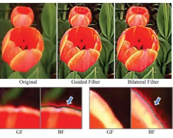
Though bilateral may not be the best noise reducing filter but it is good and simple. Also, it can be used for tone mapping, relighting and texture editing. However, the nonlinear operator is hard to compute since it is complex and spatially varying kernels. Besides, it causes staircase effect, gradient reversal, and artifact near edges as in Figure2.
Figure 2: Comparison between Bilateral and Gauss Filter with increasing spatial and intensity parameter [3]
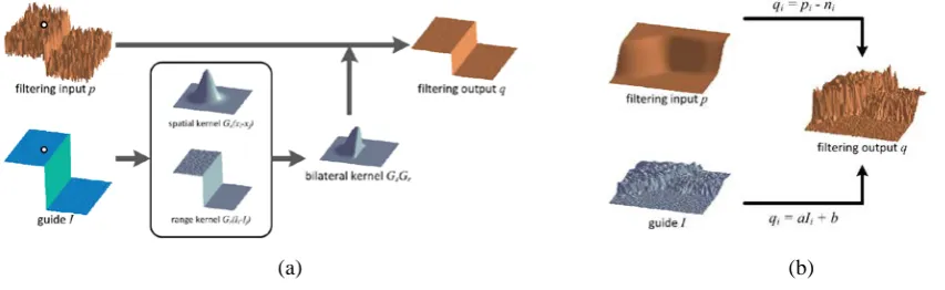
2.2.Guided Image Filtering
Guided image filter [5] is an edge preserving smoothing filter, which output is locally a linear transform of the guidance image. It has good edge-preserving smoothing properties like bilateral filter but it solves the unwanted problems which occurs in bilateral filter as in Figure3.
(a) (b)
Figure 3: (a) Bilateral Filter Process and (b) Guided Filter Process
𝑞𝑞𝑖𝑖=𝑎𝑎𝑘𝑘𝐼𝐼𝑖𝑖+𝑏𝑏𝑘𝑘,∀𝑖𝑖 ∈ 𝜔𝜔𝑘𝑘,𝑤𝑤ℎ𝑒𝑒𝑒𝑒𝑒𝑒 �𝑎𝑎𝑘𝑘= 1
|𝜔𝜔|∑𝑖𝑖∈𝜔𝜔𝑘𝑘𝐼𝐼𝑖𝑖𝑝𝑝𝑖𝑖− 𝜇𝜇𝑘𝑘𝑝𝑝̅𝑘𝑘 𝜎𝜎𝑘𝑘2+𝜖𝜖 𝑏𝑏𝑘𝑘=𝑝𝑝̅ − 𝑎𝑎𝑘𝑘𝜇𝜇𝑘𝑘
(4)
In Eq.4, 𝜇𝜇𝑘𝑘 and 𝜎𝜎𝑘𝑘2 are the mean and variance of 𝐼𝐼 in𝜔𝜔𝑘𝑘, |𝜔𝜔| is the number of pixels in 𝜔𝜔𝑘𝑘 and 𝑝𝑝̅𝑘𝑘 is the mean of 𝑝𝑝 in𝜔𝜔𝑘𝑘.
We can also model the output 𝑞𝑞 as the input 𝑝𝑝 subtracting unwanted components 𝑛𝑛 as follows:
𝑞𝑞𝑖𝑖=𝑝𝑝𝑖𝑖− 𝑛𝑛𝑖𝑖 (5)
There are two cases in an input filter that should be consider which are "high variance" region and "flat patch". The idea of guided filter is that it determine "what is an edge that should be preserved"; hence, guided filter keep the high variance patch while the flat patch is smoothed which results in its good edge-preserving property. Not only guided filter can preserve edges, it can also preserve gradient and transfer structure. Guided image filter can be fast implemented with the following Alg.1 as in [5].
Table 3
Algorithm 1: Guided Image Filtering
Input:
𝑝𝑝: filtering input image 𝐼𝐼: guidance image r: radius
𝜖𝜖: regularization
Output:
q: filtering output image
Begin
1. 𝑚𝑚𝑒𝑒𝑎𝑎𝑛𝑛𝐼𝐼 =𝑓𝑓𝑚𝑚𝑚𝑚𝑚𝑚𝑚𝑚(𝐼𝐼), 𝑚𝑚𝑒𝑒𝑎𝑎𝑛𝑛𝑃𝑃=𝑓𝑓𝑚𝑚𝑚𝑚𝑚𝑚𝑚𝑚(𝑃𝑃)
2. 𝑣𝑣𝑎𝑎𝑒𝑒𝐼𝐼=𝑐𝑐𝑐𝑐𝑒𝑒𝑒𝑒𝐼𝐼− 𝑚𝑚𝑒𝑒𝑎𝑎𝑛𝑛𝐼𝐼.∗ 𝑚𝑚𝑒𝑒𝑎𝑎𝑛𝑛𝐼𝐼, 𝑐𝑐𝑐𝑐𝑣𝑣𝐼𝐼𝑝𝑝=𝑐𝑐𝑐𝑐𝑒𝑒𝑒𝑒𝐼𝐼𝑝𝑝− 𝑚𝑚𝑒𝑒𝑎𝑎𝑛𝑛𝐼𝐼.∗ 𝑚𝑚𝑒𝑒𝑎𝑎𝑛𝑛𝑝𝑝
3. 𝑎𝑎= 𝑐𝑐𝑐𝑐𝑐𝑐𝐼𝐼𝑝𝑝
𝑐𝑐𝑚𝑚𝑎𝑎𝐼𝐼+𝜖𝜖 , 𝑏𝑏=𝑚𝑚𝑒𝑒𝑎𝑎𝑛𝑛𝑝𝑝− 𝑎𝑎.∗ 𝑚𝑚𝑒𝑒𝑎𝑎𝑛𝑛𝐼𝐼
4. 𝑚𝑚𝑒𝑒𝑎𝑎𝑛𝑛𝑚𝑚=𝑓𝑓𝑚𝑚𝑚𝑚𝑚𝑚𝑚𝑚(𝑎𝑎) , 𝑚𝑚𝑒𝑒𝑎𝑎𝑛𝑛𝑏𝑏=𝑓𝑓𝑚𝑚𝑚𝑚𝑚𝑚𝑚𝑚(𝑏𝑏) 5. 𝑞𝑞=𝑚𝑚𝑒𝑒𝑎𝑎𝑛𝑛𝑚𝑚.∗ 𝐼𝐼+𝑚𝑚𝑒𝑒𝑎𝑎𝑛𝑛𝑏𝑏
End
Figure 4: Detail enhancement comparing with Bilateral Filter with 𝑒𝑒 = 16,𝜖𝜖 = 0.12 for Guided Filter , and $𝜎𝜎𝑠𝑠 = 16,𝜎𝜎𝑎𝑎 = 0.1 for Bilateral Filter. [5]
In the Figure4, we can clearly see that guided image can avoid staircase effect and artifact that bilateral filter has. The result got from guided image is much better than the one got from bilateral filter.
Figure 5: The halo artifacts with𝑒𝑒= 16, $𝜖𝜖= 0.42 for guided filter,𝜎𝜎𝑠𝑠= 16,𝜎𝜎𝑎𝑎= 0.4 for bilateral filter.[5]
To sum up, guided filter has a 𝑂𝑂(𝑁𝑁) time non-approximate algorithm, independent of the window radius and the intensity range. Also, it is easily implement and avoid staircase effect and artifacts. It is good to be applied in feathering, matting, single image haze removal and joint up sampling. However, despite its advantage, guided filter also has its own limitation which is the exhibit halos near some edges when the image is being smoothing which is shown in Figure5.
2.3.Non-linear variational methods with Total variational denoise
The total variational method is first mentioned in the inverse problem when proposing regularizing criteria. It is based on the principle that signal has smooth details. So, denoise becomes the minimization problem, which finds a image in set of all images with bounded variation. It is applied effectively in noise reduction with smoothing image but preserving the edges [6].
The original image can be approximated by ideal and noise image as
where 𝑓𝑓 is noisy image, 𝑢𝑢 is ideal image and 𝑛𝑛 is noise image which shows as Gaussian distribution with mean 0.
Observing that 𝑢𝑢 has smooth in details, Rudin and his colleagues [6] proposes the regularizing constraint for ensuing existing unique solution in an ill-posed problem for Eq.[6] as
𝑚𝑚𝑖𝑖𝑛𝑛
𝑢𝑢∈𝐵𝐵𝐵𝐵(𝛺𝛺)�|𝛻𝛻𝑢𝑢(𝑥𝑥)|𝑑𝑑𝑥𝑥 𝛺𝛺
(7)
where first constraint assumes Gaussian Noisy with mean 0 as
� 𝑢𝑢(𝑥𝑥)𝑑𝑑𝑥𝑥 𝛺𝛺
=� 𝑓𝑓(𝑥𝑥)𝑑𝑑𝑥𝑥 𝛺𝛺
(8)
and second constraint expresses noisy derivation 𝜎𝜎 as
�|𝑢𝑢(𝑥𝑥)− 𝑓𝑓(𝑥𝑥)|2 𝛺𝛺
𝑑𝑑𝑥𝑥=𝜎𝜎2|𝛺𝛺|
(9)
In [7], Chambolle And his colleagues changed Eq.[7] into the following unconstrained minimization problem as
𝑚𝑚𝑖𝑖𝑛𝑛
𝑢𝑢∈𝐵𝐵𝐵𝐵(𝛺𝛺)�|𝛻𝛻𝑢𝑢|𝑑𝑑𝑥𝑥+ 𝜆𝜆
2‖𝑢𝑢 − 𝑓𝑓‖22𝑑𝑑𝑥𝑥 𝛺𝛺
(10)
where first term is the smoothness term, second term is data term to evaluate the accuracy of data and 𝜆𝜆 is regularization constant.
Depend on normalization for the smoothness term, there are two model energy. First, ROF (Rudin, Osher and Fatemi) model uses 𝐿𝐿1 normalization in the smoothness term as in Eq.10. Second, TV-L1 model uses 𝐿𝐿2 normalization in data term as
𝑚𝑚𝑖𝑖𝑛𝑛
𝑢𝑢∈𝐵𝐵𝐵𝐵(𝛺𝛺)�|𝛻𝛻𝑢𝑢|𝑑𝑑𝑥𝑥+𝜆𝜆‖𝑢𝑢(𝑥𝑥)− 𝑓𝑓‖ 𝑑𝑑𝑥𝑥 𝛺𝛺
(11)
TV-L1 and ROF models are the specific cases in general minimization energy problem [7, 13, 14], which defined as
𝑚𝑚𝑖𝑖𝑛𝑛𝑥𝑥 𝐵𝐵(𝐾𝐾𝑥𝑥) +𝐺𝐺𝑥𝑥 (12)
𝐵𝐵(𝐾𝐾𝑥𝑥)≜ �|𝛻𝛻𝑢𝑢| (13)
𝐺𝐺𝑅𝑅𝑅𝑅𝑅𝑅≜ �𝜆𝜆2‖𝑥𝑥 − 𝑓𝑓‖2 (14)
𝐺𝐺𝑇𝑇𝐵𝐵−𝐿𝐿1≜ � 𝜆𝜆‖𝑥𝑥 − 𝑓𝑓‖ (15)
Applying the Legendre-Fenchel transformation for 𝐵𝐵 with any 𝑝𝑝𝜖𝜖𝑋𝑋, we obtain the dual formula 𝐵𝐵∗ of 𝐵𝐵 in Eq.12 as
𝐵𝐵∗(𝑝𝑝) =𝑠𝑠𝑢𝑢𝑝𝑝
𝑥𝑥∈𝑋𝑋〈𝑝𝑝,𝑥𝑥〉 − 𝐵𝐵(𝑋𝑋) (16)
Similarly, applying the transformation for 𝐵𝐵∗ where 𝐵𝐵 and 𝐵𝐵∗ are the convex function, we obtain the formula below:
𝐵𝐵=𝐵𝐵∗∗(𝑝𝑝) =𝑠𝑠𝑢𝑢𝑝𝑝
𝑥𝑥∈𝑋𝑋〈𝑝𝑝,𝑥𝑥〉 − 𝐵𝐵 ∗(𝑋𝑋)
(17)
Applying the above formula to 𝐵𝐵, we get the saddle formula as follows:
min𝑥𝑥 max𝑝𝑝 𝐵𝐵(𝐾𝐾𝑥𝑥,𝑝𝑝) +𝐺𝐺𝑥𝑥− 𝐵𝐵∗(𝑝𝑝) (18)
in which
𝐵𝐵∗(𝑝𝑝) =𝜎𝜎
𝑃𝑃(𝑝𝑝) =�+0∞ 𝑝𝑝 ∉ 𝑃𝑃𝑝𝑝 ∈ 𝑃𝑃 (19)
where 𝑃𝑃= {𝑝𝑝:∀𝑖𝑖‖𝑝𝑝𝑖𝑖‖ ≤1}
In primal-dual algorithm, we define proximity operator which is equivalent to implicit gradient descent step, as below
(𝐼𝐼+𝜏𝜏𝜏𝜏𝐵𝐵)−1(𝑥𝑥) =𝑎𝑎𝑒𝑒𝑎𝑎𝑚𝑚𝑖𝑖𝑛𝑛 𝑥𝑥
1
2‖𝑦𝑦 − 𝑥𝑥‖2+𝜏𝜏𝐵𝐵(𝑦𝑦) (20)
To implement Primal-Dual algorithm, 𝐵𝐵∗ and 𝐺𝐺 for ROF and TV-L1 are calculated as below
(𝐼𝐼+𝜎𝜎𝜏𝜏𝐵𝐵∗)−1(𝑝𝑝) = 𝑝𝑝
𝑚𝑚𝑎𝑎𝑥𝑥(‖𝑝𝑝‖, 1) (21)
(𝐼𝐼+𝜏𝜏𝜏𝜏𝐺𝐺𝑅𝑅𝑅𝑅𝑅𝑅)−1(𝑥𝑥) =𝑥𝑥1 ++𝜆𝜆𝜏𝜏𝑓𝑓𝜆𝜆𝜏𝜏 (22)
(𝐼𝐼+𝜏𝜏𝜏𝜏𝐺𝐺𝑇𝑇𝐵𝐵−𝐿𝐿1)−1(𝑥𝑥) =�
𝑥𝑥 − 𝜆𝜆𝜎𝜎 𝑥𝑥>𝑓𝑓+𝜆𝜆𝜎𝜎 𝑥𝑥+𝜆𝜆𝜎𝜎 𝑥𝑥<𝑓𝑓 − 𝜆𝜆𝜎𝜎 𝑓𝑓 |𝑥𝑥 − 𝑓𝑓|≤ 𝜆𝜆𝜎𝜎
Table 4
Algorithm 2: Primal Dual Algorithm
Data
+ Step size 𝜎𝜎> 0, 𝜏𝜏> 0 + 𝜎𝜎𝜏𝜏𝐿𝐿2< 1, where 𝐿𝐿=‖𝐾𝐾‖ + 𝜃𝜃= 1
+ 𝑋𝑋: Input
Begin
1. 𝑥𝑥𝑖𝑖=𝑋𝑋 2. 𝑝𝑝𝑖𝑖=∇𝑥𝑥𝑖𝑖
3. while not convergence or not enough iteration do
4. 𝑝𝑝𝑖𝑖= (𝐼𝐼+𝜎𝜎𝜏𝜏𝐵𝐵∗)−1(𝑝𝑝𝑖𝑖+𝜎𝜎𝐾𝐾𝑥𝑥𝑖𝑖) % Eq.21 5. 𝑥𝑥�𝑖𝑖= (𝐼𝐼+𝜏𝜏𝜏𝜏𝐺𝐺)−1(𝑥𝑥𝑖𝑖− 𝜏𝜏𝐾𝐾𝑇𝑇𝑝𝑝𝑖𝑖) % Eq.22 or 23 6. 𝑥𝑥𝑖𝑖=𝑥𝑥�𝑖𝑖+𝜃𝜃(𝑥𝑥�𝑖𝑖− 𝑥𝑥𝑖𝑖)
End
3.Frequency Domain using Wavelet Shrinkage Denoising
Wavelet shrinkage denoising [8] is considered a non-parametric method which attempts to remove noise and retain signal regardless of the frequency content of the signal. The basic idea behind this techniques is to use wavelets to transform the data into a different basis, where "large" coefficients correspond to the signal while "small" ones represent mostly noise. The wavelet coefficients are suitably modified and the denoised data is obtained by an inverse wavelet transform of the modified coefficients.
Let 𝒀𝒀, 𝑿𝑿 and 𝜀𝜀 denote the observed data, the noiseless data and the error matrices respectively. The three main steps of denoising using the wavelet shrinkage technique are as follows:
Calculate the wavelet coefficient matrix 𝒘𝒘 by applying a wavelet transform 𝑾𝑾 to the data:
𝒘𝒘=𝑾𝑾𝒀𝒀=𝑾𝑾𝑿𝑿+𝑾𝑾𝜀𝜀 (24)
• Modify the detail coefficients to obtain the estimate 𝒘𝒘 of the coefficients of 𝑿𝑿:
𝒘𝒘 ⟶ 𝒘𝒘� (25)
𝑿𝑿�=𝑾𝑾−1𝒘𝒘� (26)
Figure 6: (left) Noisy "Lena" image with 𝜀𝜀= 20 and (right) result output provided by Wavelet Shrinkage [8]
Observing Figure[6], it notes that the noise is removed yet the detail of the image is not smooth compared to other spatial filters. However, the color contrast is not consistent as well as the computation complexity is high. Also, in some cases, wavelet shrinkage create noticeable artifact that can considerably degrade the image.
4.Integrated Spatial and Frequency Domain
4.1.Dual domain image denoising
Dual domain image denoising (DDID) [9] is an iterative denoising method which combines both spatial and transform domains. Since each domain has its advantages and shortcomings, this combination complements and solves the problems that effects on the result output.
Before DDID, there are several state-of-art approaches which combine both domain such as BM3D [15], shape-adaptive BM3D (SA-BM3D) [16] and BM3D with shape-shape-adaptive principal component analysis (BM3D-SAPCA) [10]. They denoise based on block-matching which introduces visible artifacts in homogeneous regions, expressing as low-frequency noise. Also, they are sophisticated which pay for the high quality with implementation complexity [11]. DDID offers a simpler way to implement yet competes BM3D in quality. It combines two popular filters for two domains. For the spatial domain, the bilateral filter is used to preserve features like edges; however, it has difficulties preserving low contrast details. For the transform domain, short time Fourier transform [17] with wavelet shrinkage [8, 18-20] is applied to preserve good detail though it suffers from ringing artifacts near steep edges.
Given a noise-contaminated image 𝑦𝑦=𝑥𝑥+𝜂𝜂 with a stationary variance 𝜎𝜎2=𝑉𝑉𝑎𝑎𝑒𝑒[𝜂𝜂], the goal of DIDD is to estimate the original image 𝑥𝑥. The image is separated into two layers which are denoised separately. The high-contrast layer is bilateral filtered and the low-high-contrast layer is denoised using wavelet shrinkage. Thus, the original image can be approximated by the sum of two denoised layers as
𝑥𝑥�=𝑠𝑠̃+𝑆𝑆̃ (27)
where 𝑠𝑠̃ and 𝑆𝑆̃ are the denoised high-contrast and low-contrast images.
In the first step, the denoised high-contrast values 𝑠𝑠̃𝑝𝑝 for a pixel 𝑝𝑝 is computed using a joint bilateral filter [3].
The joint bilateral uses the guide image 𝑎𝑎 to filter the noisy image y. The bilateral kernel is defined over a square neighborhood window 𝒩𝒩𝑝𝑝 centered on every pixel 𝑝𝑝 with window radius 𝑒𝑒. The parameter 𝜎𝜎𝑠𝑠 and 𝛾𝛾𝑎𝑎 shape the spatial and range kernels respectively. The two denoised image high-contrast images is obtain as following:
𝑎𝑎�𝑝𝑝=
�𝑞𝑞∈𝒩𝒩𝑝𝑝𝑘𝑘𝑝𝑝,𝑞𝑞𝑎𝑎𝑞𝑞 �𝑞𝑞∈𝒩𝒩𝑝𝑝𝑘𝑘𝑝𝑝,𝑞𝑞
(28)
𝑠𝑠̃𝑝𝑝=
�𝑞𝑞∈𝒩𝒩𝑝𝑝𝑘𝑘𝑝𝑝,𝑞𝑞𝑦𝑦𝑞𝑞 �𝑞𝑞∈𝒩𝒩𝑝𝑝𝑘𝑘𝑝𝑝,𝑞𝑞
(29)
where the bilateral kernel is
𝑘𝑘𝑝𝑝,𝑞𝑞=𝑒𝑒 −|𝑝𝑝−𝑞𝑞|2
2𝜎𝜎𝑠𝑠2 𝑒𝑒−
(𝑔𝑔𝑝𝑝−𝑔𝑔𝑞𝑞)2
𝛾𝛾𝑟𝑟𝜎𝜎𝑠𝑠2 (30)
In the second step, in the transform domain, with the wavelet shrinkage, the low contrast signals are take out by taking off the bilaterally filtered values 𝑎𝑎�𝑝𝑝 and 𝑠𝑠̃𝑝𝑝 from 𝑎𝑎𝑞𝑞 and 𝑦𝑦𝑞𝑞, followed by multiplication with the range
kernel of Eq. 30. Then, the STFT is performed to transition these low-contrast signals to the frequency domain. The resulting coefficients𝐺𝐺𝑝𝑝,𝑓𝑓, and 𝑆𝑆𝑝𝑝,𝑓𝑓, are presented for frequencies 𝑓𝑓 in the frequency window ℱ𝑝𝑝 with the
same size as 𝒩𝒩𝑝𝑝.
𝐺𝐺𝑝𝑝,𝑓𝑓= � 𝑒𝑒−𝑖𝑖2𝜋𝜋(𝑞𝑞−𝑝𝑝).𝑓𝑓/(2𝑎𝑎+1)𝑘𝑘𝑝𝑝,𝑞𝑞�𝑎𝑎𝑞𝑞− 𝑎𝑎�𝑝𝑝� 𝑞𝑞∈𝒩𝒩𝑝𝑝
(31)
𝑆𝑆𝑝𝑝,𝑓𝑓= � 𝑒𝑒−𝑖𝑖2𝜋𝜋(𝑞𝑞−𝑝𝑝).𝑓𝑓/(2𝑎𝑎+1)𝑘𝑘𝑝𝑝,𝑞𝑞�𝑦𝑦𝑞𝑞− 𝑠𝑠̃𝑝𝑝� 𝑞𝑞∈𝒩𝒩𝑝𝑝
(32)
𝜎𝜎𝑝𝑝,𝑓𝑓2 =𝜎𝜎2 � 𝑘𝑘𝑝𝑝,𝑞𝑞2 𝑞𝑞∈𝒩𝒩𝑝𝑝
(33)
In the last step, shrinkage factors like to the bilateral filter range kernel. For the wavelet shrinkage factor 𝐾𝐾𝑝𝑝,𝑓𝑓, the signal needs keeping and the noise needs discarding:
𝐾𝐾𝑝𝑝,𝑓𝑓=𝑒𝑒 −𝛾𝛾𝑓𝑓𝜎𝜎𝑝𝑝,𝑓𝑓
2
|𝐺𝐺𝑝𝑝,𝑓𝑓|2 (34)
The shrinkage factors 𝐾𝐾𝑝𝑝,𝑓𝑓 uses the spectral guide 𝐺𝐺𝑝𝑝,𝑓𝑓, and the wavelet shrinkage parameter 𝛾𝛾𝑓𝑓 shows a similar
part as the bilateral range parameter 𝛾𝛾𝑎𝑎. And the low-contrast value is yielded as following:
𝑆𝑆̃𝑝𝑝=|ℱ1𝑝𝑝| � 𝐾𝐾𝑝𝑝,𝑓𝑓𝑆𝑆𝑝𝑝,𝑓𝑓 𝑓𝑓∈ℱ𝑝𝑝
(35)
Dual domain image denoise can be fast implemented as in [9].
4.2.Nonlocal dual denoising
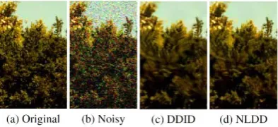
DDID provides better quality of denoised output as well as a simpler way to implement denoising method in both spatial and transform domains than any other state-of-art algorithms sharing the same idea. However, its processing time is slow and it also causes strong frequency domain artifacts unexpectedly. A later approach named Nonlocal Dual Denoising (NLDD) [12] has overcome those drawbacks.
Figure 8: Non-local dual denoising process
Figure 9: A detail of the artifacts produced by DDID and the corresponding result of NLDD. In this example𝜎𝜎= 30 [12]
5.Experiments and Discussions
5.1.Evaluation Measures
MSE (Mean-Square Error) is the average of the squares of the errors about difference between original image and restored image
𝑀𝑀𝑆𝑆𝑀𝑀=𝑚𝑚𝑛𝑛 �1 𝑚𝑚−1
𝑖𝑖=0
�[𝐼𝐼(𝑖𝑖,𝑗𝑗)− 𝐾𝐾(𝑖𝑖,𝑗𝑗)]2 𝑚𝑚−1
𝑗𝑗=0
(36)
where 𝐼𝐼 and 𝐾𝐾 respectively are the original image and restored image with size 𝑚𝑚 ×𝑛𝑛.\\
RMSE (Root-mean-square error) is dervied from MSE as below
𝑅𝑅𝑀𝑀𝑆𝑆𝑀𝑀=√𝑀𝑀𝑆𝑆𝑀𝑀 (37)
PSNR (Peak Signal to Noise Ratio) is a term used to calculate the ratio between the maximum energy value of a signal and the noise energy influences the accuracy of the information. Because there are many wide variation signals, the PSNR is usually represented by the dB unit. The bigger the PSNR is, the better the image is. The formula is used to calculate PSNR as below
𝑃𝑃𝑆𝑆𝑁𝑁𝑅𝑅= 10𝑙𝑙𝑐𝑐𝑎𝑎10�𝑀𝑀𝑀𝑀𝑋𝑋𝐼𝐼 2
𝑀𝑀𝑆𝑆𝑀𝑀 � (38)
where 𝑀𝑀𝑀𝑀𝑋𝑋𝐼𝐼 is the maximum value of the pixel on the image.
5.2.Noise models
probability density function p of the Gaussian random variable z is given by the formula [4]:
𝑝𝑝(𝑧𝑧) = 1
√2𝜋𝜋𝜎𝜎𝑒𝑒−(𝑧𝑧−𝜇𝜇)
2
/2𝜎𝜎2 (38)
where 𝑧𝑧 represents the grey level, 𝜇𝜇 the mean value and 𝜎𝜎 the standard deviation.
5.3.Experiments
In paper, we implement benchmark for denoise methods introduced above. Bilateral method has code from OpenCV. Guided image filter implements from guide of author in [5]. In Guided image filter, we use guide images from bilateral filter and original filter. With TV-L1, we implements from [13]. Lastly, we use reports from [12] on homepage to take results of DDID and NLDD methods.
Table 1 shows comparison methods such bilateral filter, guided image filter using bilateral filter and original input for guided image:
Table 1: PSNR comparision among noise image, Bilateral filter, Guided image filter with guide image using
Bilater and original image
Noise Bilateral Bilateral Guide Original Guide
Alley 11.6 20.51 20.94 24.44
Computer 11.96 20 19.99 24.36
Dice 11.67 22.44 24.51 36.84
Flowers 12.39 20.29 20.66 31.28
Girl 11.69 22.8 25.08 30.3
Traffic 11.78 19.83 19.74 23.35
Trees 11.82 18.3 17.63 19.41
Table 2 shows results of remain methods:
Table 2: PSNR comparision among TV-L1, Dual-domain image denoise and non-local dual denoise method
TVL1 DDID NLDD
Alley 22.16 25.3 25.23
Computer 21.67 25.95 25.91
Dice 25.66 32.33 33.54
Flowers 21.84 28.81 29.46
Girl 26.47 32.11 32.94
Traffic 21.41 24.63 24.77
From Table 1 and 2, DDID and NLDD methods have results better than remain methods. They take advantages of spatial and transform domain in denoise. Besides, we also see that images with many details such as Trees image, Traffic image will take lower results for all methods as Figure10.
Figure10: Comparision PSNR between denoise methods
6.Conclusions
To sum up, paper makes a survey for denoise methods. Bilateral filter, guided image filter and total variational methods process by spatial domain. In which, total variational method has good result more than remain methods.
Besides, the results also shows NLDD, DDID are effective methods in denoise with not only hybrid approach but also spatial methods. From the survey, denoise also has many challenges when denoising on images too small details.
References
[1] M. Motwani, M. Gadiya, R. Motwani, and F. Harris Jr, “Survey of image denoising techniques,” in Proceedings of GSPx, 2004, pp. 27 30.
[2] C. Tomasi and R. Manduchi, “Bilateral filtering for gray and color images,” Sixth International Conference on Computer Vision (IEEE Cat. No.98CH36271), pp. 839–846, 1998. [Online]. Available: http://ieeexplore.ieee.org/document/710815/
[4] R. C. Gonzalez and R. E. Woods, Digital Image Processing (3rd Edition). Upper Saddle River, NJ, USA: Prentice-Hall, Inc., 2006.
[5] K. He, J. Sun, and X. Tang, “Guided image filtering,” IEEE Transactions on Pattern Analysis and Machine Intelligence, vol. 35, no. 6, pp. 1397–1409, 2013.
[6] L. I. Rudin, S. Osher, and E. Fatemi, “Nonlinear total variation based noise removal algorithms,” Phys. D, vol. 60, no. 1-4, pp. 259–268, 1992.
[7] A. Chambolle, V. Caselles, D. Cremers, M. Novaga, and T. Pock, “An Introduction to Total Variation for Image Analysis,” Theoretical foundations and numerical methods for sparse recovery, vol. 9, pp. 263–340, 2010.
[8] I. K. Fodor and C. Kamath, “Denoising through wavelet shrinkage: an empirical study,” Journal of Electronic Imaging, vol. 12, no. 1, pp. 151–160, 2003.
[9] C. Knaus and M. Zwicker, “Dual-domain image denoising,” IEEE International Conference on Image Processing, ICIP 2013 Proceedings, no. 4, pp. 440–444, 2013.
[10] K. Dabov, R. Foi, V. Katkovnik, and K. Egiazarian, “BM3D image denoising with shape-adaptive principal component analysis,” Proc. Workshop on Signal Processing with Adaptive Sparse Structured Representations, p. 6, 2009.
[11] M. Lebrun, “An Analysis and Implementation of the BM3D Image Denoising Method,” Image Processing On Line, vol. 2, no. May, pp.175–213, 2012. [Online]. Available: http://www.ipol.im/pub/art/2012/l- bm3d/?utm_source=doi
[12] N. Pierazzo, M. Lebrun, M. E. Rais, J. M. Morel, and G. Facciolo, “Non-local dual image denoising,” in 2014 IEEE Internationa Conference on Image Processing, ICIP 2014, 2014, pp. 813–817.
[13]A.Mordvintsev.(2013)Rofandtv-l1denois-ingwithprimal-dualalgorithm.[Online].Available: https://github.com/znah/notebooks/blob/master/TV_denoise.ipynb
[14] J. Duran, B. Coll, and C. Sbert, “Chambolle’s Projection Algorithm for Total Variation Denoising,” Image Processing On Line, vol. 2013, pp.311–331, 2013.
[15] K. Dabov, A. Foi, V. Katkovnik, and K. Egiazarian, “Image restoration by sparse 3D transform-domain collaborative filtering,” Proceedings of SPIE-IS&T, Image Processing: Algorithms and Systems VI, San Jose, California, USA, 28 January 2008, vol. 6812, no. 213462, p. 12, 2008.
[17] J. Allen, “Short term spectral analysis, synthesis, and modification by discrete Fourier transform,” Acoustics, Speech and Signal Processing, IEEE Transactions on, vol. 25, no. 3, pp. 235–238, 1977.
[18] D. L. Donoho, I. M. Johnstone, G. Kerkyacharian, and D. Picard, “Wavelet Shrinkage: Asymptopia?” Journal of the Royal Statistical Society. Series B (Methodological), vol. 57, no. 2, pp. 301–369, 1995. [Online]. Available: http://statweb.stanford.edu/ imj/WEBLIST/1995/asymp.pdf
[19] X. Zong, “De-noising and contrast enhancement via wavelet shrinkage and nonlinear adaptive gain,” Proceedings of SPIE, vol. 2762, pp. 566–574, 1996. [Online]. Available: http://link.aip.org/link/?PSI/2762/566/1&Agg=doi
![Figure 1: Bilateral filter for smoothing an input image [3]](https://thumb-us.123doks.com/thumbv2/123dok_us/8398442.1685576/3.595.207.386.333.453/figure-bilateral-filter-smoothing-input-image.webp)