Modeling And Analysis Of Turning Process On
Lathe Machine By Taguchi And Anova Approach
Manoj Modi, Gopal Agarwal, V.Patil, Ashish Khare, Saloni Shukla, Advitiya Sankhala
Abstract: In the today‘s competitive era, it is very important to an edge over the others to survive and flourish. One of the easiest yet most complicated
areas to expertise is ‗fast delivery‘ and to obtain that the cycle time has to be reduced. Keeping this in mind certain investigations are carried out to increase the material removal rate. This research work explains the effects of certain lathe parameters namely Speed, Feed and Depth of Cut on the output parameter Material Removal Rate. A mild steel test piece is taken and different experiments are conducted on it by a nine foot conventional lathe machine by changing the input parameters using Taguchi methodology. Taguchi method is used to formulate the experimental layout. A Taguchi L9 design of experiment (DOE) and the analysis of variance (ANOVA) is applied to analyze the effect of each parameter on the response. Mathematical formula is also developed among the Speed, Feed and Depth of Cut and MRR. It will be found that these parameters have a significant influence on machining characteristic metal removal rate.
Index Terms: Speed, Feed, Depth of Cut, Taguchi, ANOVA, and MRR.
—————————— ——————————
1.
INTRODUCTION
Conventional machines are manually controlled by hand wheels or levers. The machines take more time to make one component and needs one man one machine for supervision. This make the manufactured product costly as well as quality of the product vary according to man expertise on that machine, which is not feasible in this competitive environment. The development of manufacturing technologies to improve machining and obtain high productivity has become a very important goal in modern industry. The challenge of modern machining industries is mainly focused on the achievement of high quality, in terms of work piece dimensional accuracy, surface finish, high production rate, less wear on the cutting tools, economy of machining in terms of cost saving and increase the performance of the product with reduced environmental impact.
1.1 MATERIALS AND METHODS
Turning operation is one of the most basic machining processes in which the part is rotated while a single point cutting tool is moved parallel to the axis of rotation to cut and finish the work piece to obtain a desired shape and size, it can be done externally and internally (boring) on the work-piece and can be optimised through various parameters like cutting speed, depth of cut, feed value, material removal rate, power drawn, etc. For finding the effects of LATHE machine parameters like speed (RPM), feed (mm) and depth of cut (mm) on material removal rate, a mild steel work piece was taken. The work piece weighed 1.5 kgs with a solid cylindrical
The outer diameter was 40.6 mm. We then used a high speed steel (HSS) single point cutting tool to carry on with the experiment. The idea behind deciding material of the single point cutting tool was that it is harder than mild steel and is easily available in the market. We then carried our experiment with the help of L9 orthogonal array of Taguchi Approach.
1.2 Introduction to Taguchi Methodology
Taguchi Method was proposed by Genichi Taguchi, a Japanese quality management consultant. The method explores the concept of quadratic quality loss function and uses a statistical measure of performance called signal to noise (S/N) ratio. Taguchi method is usually used in an analysis that uses a number of factors. When the total factors have been more than two, the number of experiment also will increase, and then the solution will be used Taguchi method. Taguchi Methods is a system of cost driven quality engineering that emphasizes on the effective application of engineering strategies rather than advanced statistical technique. It includes both upstream and shop floor quality engineering. Upstream methods efficiently use small scale experiments to reduce variability and find cost effective, robust designs for large scale production and the market place. Shop floor techniques provide cost based real time methods for monitoring and maintaining quality in production. Taguchi Methods allow a company to rapidly and accurately acquire technical information to design and produce low cost, highly reliable products and processes. Its most advanced applications allow engineers to develop flexible technology for the design and production of families of high quality products, greatly reducing research, development and delivery time. The DOE with Taguchi approach is divided into three main phases-
1. Planning phase, 2. Conducting phase, and 3. Analysis phase
1.3 Principle of ANOVA Approach
The basic principle of ANOVA is to test for differences among the means of the populations by examining the amount of variation within each of these samples, relative to the amount of variation between the samples. In terms of variation within the given population, it is assumed that the values of (Xij) differ from the mean of this population only because of random effects i.e., there are influences on (Xij) which are unexplainable, whereas in examining differences between
1
_______________________________
Department of Mechanical Engineering, Acropolis Institute of Technology and Research, Indore, India.
Corresponding Author E-mail: [email protected]
Department of Mechanical Engineering,, Malaviya National Institute of Technology, Jaipur, Rajasthan, India.
Department of MechanicalEngineering, Acropolis Institute of Technology and Research, Indore, India.
populations we assume that the difference between the mean of the jth population and the grand mean is attributable to what is called a ‗specific factor‘ or what is technically described as treatment effect. Thus while using ANOVA; we assume that each of the samples is drawn from a normal population and that each of these populations has the same variance. We also assume that all factors other than the one or more being tested are effectively controlled. We further assume the absence of many factors that might affect our conclusions concerning the factor(s) to be studied. Here we have used the regression method to find out the mathematical model in each case of experimentation.
2
LITERATURE REVIEW
Many studies have been made using Taguchi Method to optimize the turning parameter. M. Nalbalt et al (2006) use L9 orthogonal array with nine total experiments, to study the performance characteristics in turning operations of AISI 1030 steel bars using Tin coated tools. Three cutting parameters namely, insert radius, feed rate, and depth of cut, are optimized with considerations of surface roughness. The experimental results demonstrate that the insert radius and feed rate are the main parameters among the three controllable factors (insert radius, feed rate and depth of cut) that influence the surface roughness in turning AISI 1030 carbon steel. W.H Yang and Y.S Tang (1998) carried out an experiment consist of eighteen combination on an engine lathe using tungsten carbide with the grade of P-10 for the machining of S45C steel bars. The cutting parameters that have been selected are cutting speed, feed rate and depth of cut with the response variable, tool life and surface roughness. Result show that cutting speed and feed rate are the significant cutting parameters for affecting tool life, while the change of the depth of cut in the range has an insignificant effect on tool life. For surface roughness, all the cutting parameters have the significant effect. The confirmation experiments then were conducted to verify the optimal cutting parameters. The improvement of tool life and surface roughness from the initial cutting parameters to the optimal cutting parameters is about 250%. E.D Kirby et al (2005) use the application of the Taguchi parameter design method to optimizing the surface finish in a turning operation. This study was conducted using samples cut from a single length of 1-in diameter 6061-T6 aluminum alloy rod. Feng and Wang [4] found that many published studies include spindle speed and feed rate, and a few included the depth of cut. Decreased feed rate has been found to generally reduce surface roughness; however, the effects of the spindle speed and depth of cut on surface roughness seem to have different interpretations by different authors [4–6].
2.1 Research Gap
On the basis of above literature we came to the conclusion that very little work has been done in the area of optimization of material removal rate using combinations of the input parameters like speed, feed and depth of cut. So we decided to focus on these by opting for mild steel as our working material through the ANOVA method and MINITAB software.
3
PROBLEM
DEFINITION/DESCRIPTION
―Machining a work piece‖ is itself a self sufficient statement which means to get the rough work piece in a desired shape and size with the desired surface finish. The end product or
the finished component of desired dimensions can be achieved by various methods and one has to choose the most suitable method for the job which is cost and time efficient. Choosing such a method or changing a predetermined method is known as optimization. Machine optimization involves the determination of efficient machining parameters such as cutting speed, feed rate and depth of cut in process planning stage. It directly impacts the production economics of machining processes in terms of meeting the minimum production cost, minimum production time, maximum production rate, and maximum production profit objectives. Therefore, to make sure that highest profit is obtained, one has to understand all these areas. In this project some of the areas like material removal rate, specimen temperature and tool wear are covered. We decided to optimize the material removal rate by changing the input parameters such as speed (RPM), feed (mm) and depth of cut. This led to change in MRR and also gave us the highest rate. Hence we could optimize the same.
3.1 Objective of the Project
Since we are focusing on the MRR in the light of 3 input parameters, our objectives are as follows:
1) To find out the changes in material removal rate when we change the speed (RPM).
2) To find out the changes in material removal rate when we change the feed input.
3) To find out the changes in material removal rate when we change the depth of cut.
4
METHODOLOGY
We have chalked out our method of working on the project as- Study of Taguchi Methodology.
Deciding and acquirement of work piece. Deciding the tool to be used.
Deciding the input parameters. Mounting the job on the lathe. Setting the input parameters.
Carrying out the experiment while changing the input values and noting down the readings. Measuring the material removed after each step. Repeating the experiment till all the values are obtained.
4.1 STUDY OF TAGUCHI METHODOLOGY
After reading various research papers present on the internet and going through other reading material we came to know about a method of experimentation known as Taguchi method. Taguchi method appeared to be the exact form of working we required and hence decided to go for it. We opted for L9 orthogonal array to conduct and represent our experiment. It is a form of experimentation in which 3 to 4 input parameters can be taken, but each parameter has to have 3 levels. L9 orthogonal array compels the user to conduct not less than 9 experiments to get the optimum readings. This satisfied our requirement completely as we had 3 input parameters, namely speed, feed and depth of cut, and also had 3 levels for each of the inputs. Our requirement to find material removal rate needed 9 experiments in all by creating constants in the input parameters one by one. This was also fulfilled by L9 orthogonal array.
An example of the array we used- 3
Experiment No. Level 1 Level 2 Level 3
1 1 1 1
2 1 1 2
3 1 1 3
4 2 2 1
5 2 2 2
6 2 2 3
7 3 3 1
8 3 3 2
9 3 3 3
This table was used to put input values and attain the output.
4.2 Deciding and acquirement of work piece
On deciding the type of the experiment we wanted to perform. The next big thing was deciding which material should be used to conduct the experiment. After doing extensive research, we picked out mild steel as our test piece material for its availability, cheap cost and wide-spread uses along the range of industries. We thought of experiment on MS as that would provide plenty of opportunities of us as well as might find optimisation methods which might be useful in other institutes too.
We then decided the dimensions of the work piece which was easy to handle and could easily be fitted in a LATHE machine, hence decided upon-
Weight- 1.5 kgs
Outer diameter- 40.6 mm
Length- 154 mm
4.3 Deciding the tool to be used
To machine a piece of mild steel solid shaft on the LATHE machine, we decided to go for single point cutting tool as it provides the desired finish and is easily available.
Now came the step in which we had to make our mind as to which tool material should be used as single point cutting tool. We settled on high speed steel (HSS) as it is harder than mild steel, gives high quality finish, is cheaper and is easily available.
4.4 DECIDING THE INPUT PARAMETERS We chose the input parameters as-
Speed- material removal rate depends directly on the RPMs of the job, hence taking speed as one of the parameters was legit.
Feed- the distance the tool has moved obviously had an effect on the material removal rate, therefore taking it as another input parameter made sense.
Depth of cut- the deeper the tool went in the work piece, the more the material was removed, so depth of cut was taken as the third parameter.
4.5 Mounting the job on the lathe
The work piece was fixed on the Lathe machine through a four-jaw chuck and centered.
4.6 SETTING THE INPUT PARAMETERS
All the input parameters were set according to L9 orthogonal array, such as-
Speed- the RPM of the job would be same as the rotational speed of the driven pulleys. This was found out by reducing the speed in accordance with the pulley diameter ratios with the pulleys connected to the motor. To change the pulley combination we pulled a lever, the belt over the pulleys slackened and we could then shift it on another pulley combination. Therefore as the motor RPM were 1940 and there were 3 pulley sets of different diameters, we were able to obtain 3 different levels of the speed. Another foolproof method of finding out the speed is to use a tachometer.
Feed- the distance the tool moved parallel to the axis of rotation was measured by starting the machine and stopping it after 1 minute. Since in each cycle the RPMs varied, we got 3 different levels of feed too.
Depth of cut- the deeper the tool went in the work piece was fixed by setting it on the LATHE machine. Hence we set it thrice with different values.
We decided on 3 levels of each input parameters as-
Parameters Level 1 Level 2 Level 3
Speed (RPM) 810 1280 1750
Feed (mm) 12.7 19.7 26.7
DOC (mm) 0.5 1.0 1.5
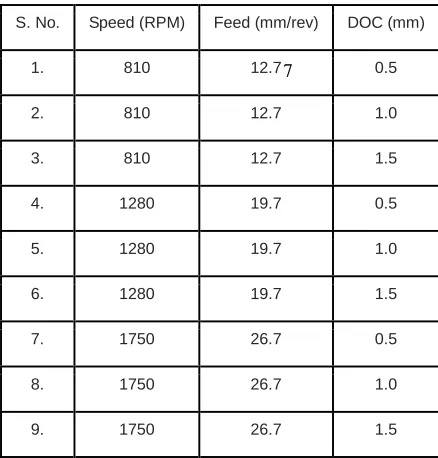
4.7 Carrying out the experiment while changing the input values and noting down the readings
With these three levels, we carried out our experiment by creating combinations of them according to L9 orthogonal array and found out the material removal rate in each case by weighing the material removed in the form of chips as-
S. No. Speed (RPM) Feed (mm/rev) DOC (mm)
1. 810 12.7 0.5
2. 810 12.7 1.0
3. 810 12.7 1.5
4. 1280 19.7 0.5
5. 1280 19.7 1.0
6. 1280 19.7 1.5
7. 1750 26.7 0.5
8. 1750 26.7 1.0
9. 1750 26.7 1.5
7 Table 1: L9 orthogonal array
5
OBSERVATIONS AND RESULT
5.1 Observations
After carrying out the experiment nine times (as we used L9 orthogonal array) with different values, we found out that the material removal rate changed as under-
S. No Speed (RPM)
Feed (mm/rev)
DOC (mm)
MRR (kg/min)
1. 810 12.7 0.5 0.006
2. 810 12.7 1.0 0.012
3. 810 12.7 1.5 0.017
4. 1280 19.7 0.5 0.009
5. 1280 19.7 1.0 0.018
6. 1280 19.7 1.5 0.027
7. 1750 26.7 0.5 0.013
8. 1750 26.7 1.0 0.026
9. 1750 26.7 1.5 0.049
5.2 Results
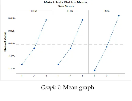
The results obtained show that material removal rate can be mathematically modeled and can be displayed with the help of MINITAB software as-
Table 4: Observations
Graph 1: Mean graph
3.0 2.5 2.0 1.5 1.0 0.05
0.04
0.03
0.02
0.01
0.00
S 0.0121610 R-Sq 35.1% R-Sq(adj) 13.5%
RPM
M
R
R
Fitted Line Plot
3.0 2.5
2.0 1.5
1.0 0.05
0.04
0.03
0.02
0.01
0.00
S 0.0104828
R-Sq 51.8%
R-Sq(adj) 35.7%
DOC
M
R
R
Fitted Line Plot
MRR = 0.00300 + 0.00483 DOC + 0.001500 DOC^2
6 CONCLUSIONS
It is found that the relation between RPM and MRR is as- Material removal rate increases with increase the speed (RPM). The regression equation is
MRR = 0.01033 - 0.00117 RPM + 0.002500 RPM^2It is found that the relation between Feed and MRR is as-
Material removal rate increases with increase the feed input. The regression equation is
MRR = 0.01033 - 0.00117 FEED + 0.002500 FEED^2
It is found that the relation between Depth of Cut and MRR is as-
Material removal rate increases with increase the depth of cut. The regression equation is
MRR = 0.00300 + 0.00483 DOC + 0.001500 DOC^2
REFERENCES
[1] Dragomir, C., & Surugiu, F. Implementing Lean in a Higher Education University. Constanta Maritime University's Annals, 18 , pp.279–282, 2013.
[2] Muammer Nalbant, H. Gökkaya, Gökhan Sur, Application of Taguchi method in the optimization of cutting parameters for surface roughness in turning, Materials and Design December 2007, 28(4):1379-1385.
[3] Yang WH, Tarng YS (1998) Design optimisation of cutting parameters for turning operations based on Taguchi method. J Mater Process Technol 84:122–129. [4] E. Daniel Kirby, Zhe Zhang, Joseph C. Chen,
Jacob Chen, Optimizing surface finish in a turning operation using the Taguchi parameter design method [5] Feng C-X, Wang X-F (2003) Surface roughness
predictive modeling: neural networks versus regression. IIE Trans 35:11–27.
[6] Davim JP (2001) A note on the determination of optimal cutting conditions on the surface finish obtained in turning using design experiments. J Mater Process Technol 116(2/3):305–308
[7] Kopac J, Bahor M, SokoviC M (2002) Optimal machining parameters for achieving the desired surface roughness in fine turning of cold pre-formed steel workpieces. Int J Mach Tools Manuf 42(6):707– 716.
3.0 2.5
2.0 1.5
1.0 0.05
0.04
0.03
0.02
0.01
0.00
S 0.0121610
R-Sq 35.1%
R-Sq(adj) 13.5%
FEED
M
R
R
Fitted Line Plot
MRR = 0.01033 - 0.00117 FEED + 0.002500 FEED^2
Graph 3: FEED Vs MRR