Accounting Conservatism,
Changes In Real Investment,
And Analysts’ Earnings Forecasts
Kyong Soo Choi, Keimyung University, South Korea
Se Joong Lee, Ph.D student, The University of Hong Kong, Hong Kong Soo Yeon Park, Korea University, South Korea
Yong Keun Yoo, Korea University, South Korea
ABSTRACT
This study examines whether sell-side analysts fully incorporate into their earnings forecasts the joint effects between accounting conservatism and changes in real investment on the quality of current earnings. Our results indicate that sell-side analysts do not fully incorporate such effects when they forecast future earnings so that they overestimate (underestimate) future earnings when current earnings are inflated (depressed) by those effects. Thus, we conclude that sell-side analysts do not recognize fully the joint effects between accounting conservatism and real activity on the earnings quality and that they need to mitigate their bias to enhance market efficiency by providing investors with a good benchmark for their earnings expectation.
Keywords: Analysts’ Earnings Forecasts; Earnings Quality; Market Efficiency
1. INTRODUCTION
his paper examines whether sell-side analysts fully incorporate into their earnings forecasts the effects of interaction between accounting conservatism and changes in real investment on the quality of current earnings. Penman and Zhang (2002) demonstrate that investors do not fully recognize the varying quality of current earnings, arising from the joint effect of accounting conservatism and changes in real investment, when they forecast future earnings. This evidence implies that the market valuations can be biased, at least, in a short term, since investors value firms without fully appreciating the quality of current earnings. Given the market’s mispricing of earnings quality, it is worthwhile to evaluate the factors which might mitigate or exacerbate the market’s mispricing. This is because the stock market’s pricing errors, i.e., the stock price’s deviation from the intrinsic value of equity, could substantially impede the efficient allocation of resources among competing stocks. Given that sell-side analysts are the most prominent information intermediaries in the capital market, we investigate whether they identify and communicate information about the quality of current earnings with investors.
Our research builds largely on the seminal study by Penman and Zhang (2002). Penman and Zhang (2002) is unique in examining how accounting methods affect the quality of reported earnings. Most of the existing studies related to this subject stress that the quality of earnings depends highly on the changes in accounting methods or estimates (Healy 1985; Beaver and Engel 1996; Moehrle 2002). Penman and Zhang (2002), on the other hand, argue that the quality of earnings can be affected by the interaction between permanent choice of accounting methods and changes in real investment, not merely by changes in accounting methods or estimates. Specifically, using their own constructed index of accounting conservatism (C-score) and earnings quality (Q-score), they empirically show that conservative accounting coupled with temporary changes in real investment does affect the quality of current earnings. Furthermore, Penman and Zhang (2002) demonstrate that investors fail to fully appreciate the effects of accounting conservatism and changes in real investment on the quality of current earnings, which leads to the market’s mispricing.
Our study extends their study by exploring whether sell-side analysts’ earnings forecasts fully incorporate such effects. So far, many accounting literature has been interested in the efficiency of analysts’ earnings forecasts and has provided mixed results on whether they can function as a signal for the market’s mispricing (e.g., Abarbanell 1991; Stickel 1991; Gleason and Lee 2003; Liu 2003; Gunny 2005). However, all of these studies examine the analysts’ ability to recognize fully the effects of accounting method choice or the effects of real activity on earnings quality individually, not simultaneously. Hence, this void of previous literature motivates us to examine whether analysts’ earnings forecasts can facilitate investors to better understand the effects of interaction between accounting conservatism and changes in real investment on the quality of current earnings.
To address this issue, we empirically examine the association between analysts’ earnings forecast errors and the index (i.e. Q score) of quality of current earnings. If analysts fully incorporate the quality of current earnings, which relates to the effect of interaction between accounting conservatism and changes in real investment on future earnings, analysts’ earnings forecast errors should not be associated with the index of quality of current earnings. Using the U.S. data for the fiscal years of 1985-2008, however, we find a significant association between analysts’ earnings forecasts errors and the index of earnings quality. This result indicates that sell-side analysts do not fully incorporate the quality of current earnings affected by the joint effect of accounting conservatism and changes in real investment on future earnings when they forecast future earnings. It implies that investors cannot fully mitigate their mispricing of such an effect by using analysts’ earnings forecast as the benchmark for their earnings expectation.
This study contributes to the growing body of evidence relating to the efficiency of analysts’ earnings forecast. Although prior research has accumulated abundant evidence with respect to the efficiency of analysts’ earnings forecasts, none of these studies examine analysts’ ability to incorporate the joint effect of permanent accounting policy (accounting conservatism) and changes in real activity (changes in real investment) on the quality of current earnings. Thus, our study may promote investors’ assessment of the usefulness or limitation of analysts’ earnings forecasts when investors make their own earnings expectation1. This study also supplements the findings provided by Penman and Zhang (2002). Our evidence suggests that even professional financial intermediaries, who may have superior ability to interpret accounting information, do not fully incorporate the joint effect of accounting conservatism and changes in real investment on future earnings. Thus, our evidence reinforces the previous findings that investors do not appear to fully understand how accounting conservatism and changes in real investment jointly affect the quality of current earnings.
The remainder of this paper is organized as follows. The next section summarizes related studies and develops our hypothesis. Section 3 describes our research method and sample selection. Section 4 presents the empirical results and Section 5 concludes.
2. BACKGROUND AND HYPOTHESIS DEVELOPMENT
The question of whether investors fully appreciate the implication of current earnings on future earnings when predicting future earnings is a matter of primary concern to accounting policy makers as well as academic researchers. A number of literature suggests that investors do not fully appreciate the implication of current earnings on future earnings when predicting future earnings (e.g., Dechow et al. 1996; Sloan 1996; Xie 2001). These findings can be viewed as one of the most prominent pieces of evidence which establish the phenomenon of market inefficiency. Note that these studies are mainly characterized by focusing on the earnings quality which is affected by the changes in accounting methods or estimates (Collins and Hribar 2000; Richardson et al. 2005; Thomas and Zhang 2002; Pincus et al. 2007). For example, if the changes in estimates of bad debts or loan loss reserves are temporary, current earnings are of poor quality since this temporary effect reverses soon. In this line of reasoning,
1 On the one hand, various previous studies provide the evidence which supports the analysts’ ability to lessen the market’s mispricing (e.g.,
current earnings seem to become more sustainable and so be of high quality when consistent accounting methods or estimates are applied.
Penman and Zhang (2002), however, substantially differ from this line of research by suggesting that the concerns on earnings quality still remain even when firms apply an accounting principle consistently. They show that even if firms implement conservative accounting permanently without changing accounting methods or estimates, temporary changes in real investment coupled with conservative accounting significantly affects the quality of current earnings. More specifically, conservative accounting reduces current earnings because it recognizes investment as expenses more than do the normal accounting. So, it builds up “hidden reserve” (hereafter, “reserve”) that might have been booked as assets under less conservative accounting and would be reported as profits when the growth of investment slows or investment declines. This phenomenon can arise from any application of conservative accounting. For example, LIFO inventory method produces higher cost of goods sold and lowers earnings, creating reserves, than FIFO inventory method. The recognition of R&D and advertisement expenses has similar effects on current earnings. That is, under conservative accounting, increase in real investment leads to lower current earnings than the ones which might have been reported by less conservative accounting, while it leads to higher future earnings. If the change in real investment is temporary, the resulting change in current earnings is also temporary and thus the current earnings become of low quality. Therefore, Penman and Zhang (2002) conclude that earnings quality can be affected by the interaction between conservative accounting and the change of real activity, as well as by the changes in accounting methods or estimates.
Furthermore, Penman and Zhang (2002) suggest that investors do not fully incorporate the joint effect of accounting conservatism and changes in real investment on future earnings when predicting future earnings. Since investors fixate on current earnings, without incorporating fully such an effect, stock price deviates from the intrinsic value of equity. Given that the market’s mispricing of current earnings severely threatens the economically efficient allocations of resources in the capital market, it is of primary importance to assess which factors might mitigate or exacerbate the market’s mispricing. Accordingly, we examine whether sell-side analysts fully incorporate into their earnings forecasts the effects of interaction between accounting conservatism and changes in real investment on the quality of current earnings.
Given the prominent role of sell-side analysts as information intermediaries in the capital market, many research pays great attention to whether analysts’ earnings forecasts can mitigate the market inefficiency. On the one hand, various studies provide the evidence which supports the analysts’ ability to lessen the market’s mispricing (e.g., Abarbanell and Bernard 1992; Frankel and Lee 1998; Lee et al. 1999; Ali et al. 2003). For example, Elgers et al. (2003) conclude that analysts’ earnings forecasts are less biased than investors’ earnings expectation in interpreting accruals. Also, Gunny (2005) suggests that analysts recognize the future earnings implications of earnings manipulation through the change of real activities while investors do not. These studies, as a whole, demonstrate that a significant portion of the market’s mispricing arises from the investors who are not able to incorporate fully information contents contained in analysts’ earnings forecasts.
On the other hand, a number of literature provides the evidence which indicates the inefficiency of analysts’ earnings forecasts (e.g., Stober 1992; Ababanell and Bushee 1997; Easterwood and Nutt 1999). Ababanell and Bushee (1997) suggest that analysts’ forecast revisions fail to impound fully all the information about future earnings contained in the fundamental signals. Bradshaw et al. (2001) suggest that analysts do not fully incorporate the lower earnings quality associated with higher accruals into their earnings forecasts. Also, Kang and Yoo (2007) argue that analysts’ earnings forecasts are more biased than the market’s earnings expectation in interpreting accruals, which is contradictory to Elgers et al. (2003). Moreover, another set of studies examines the effect of accounting conservatism on analysts’ earnings forecasts errors (Mensah et al. 2004; Louis et al. 2008; Pae and Thornton 2010). These studies provide consistent evidence that analysts’ earnings forecasts errors are systematically associated with the level of conservative accounting. These results can be interpreted as analysts forecast future earnings as if they do not fully understand the implications of conservative accounting for future earnings.
Correspondingly, the question of whether analysts fully incorporate into their earnings forecasts the effect of interaction between accounting conservatism and changes in real investment on the quality of current earnings remains unexplored.
Thus, we examine whether analysts’ earnings forecast errors are systematically associated with the quality of current earnings affected by the interaction between conservative accounting and changes in real investment. Following Penman and Zhang (2002), we construct C-score as the level of estimated reserves created by the conservative accounting relative to net operating assets. We measure the estimated reserves as the unrecorded net assets resulting from using LIFO inventory method, R&D expensing and advertising expenditures. Penman and Zhang (2002) suggest that the change in estimated reserves relative to net operating assets captures the joint effect of accounting conservatism and changes in real investment on the quality of current earnings. So, in order to measure the earnings quality, we construct the earnings quality index, i.e., the Q-score, as the change of C-score. Penman and Zhang (2002) empirically show that the Q-score has the ability to identify the effects of interaction between accounting conservatism and temporary change in real investment on current and future earnings, suggesting that the Q-score is an appropriate measure to capture the quality of earnings. More specifically, they show that a relatively higher (lower) Q-score implies current earnings that are lower (higher) than that expected in the future.
Our empirical hypothesis with respect to the association between analysts’ earnings forecasts errors and the Q-score is straightforward. We hypothesize that analysts’ earnings forecasts reveal a greater pessimistic (optimistic) bias when the level of Q-score is relatively high (low), or a positive association between analysts’ earnings forecasts errors (measured as the difference between actual earnings and forecasted earnings) and the level of Q-score. If so, it indicates that analysts fail to incorporate fully into their earnings forecasts the effect of interaction between accounting conservatism and changes in real investment on earnings quality. More formally, our alternative hypothesis proceeds as follows:
H1: Analysts’ earnings forecasts errors are positively associated with the level of Q-score.
3. RESEARCH DESIGN
3.1 Measurement of Earnings Quality
We adopt the Q-score constructed by Penman and Zhang (2002) as the index to measure the level of earnings quality, which incorporates the joint effects between accounting conservatism and changes in real investment on earnings quality. Following Penman and Zhang (2002), we regard earnings quality as low when Q-score is either excessively high or excessively low. The Q-Q-score consists of two subordinated measures, QA and QB. QA is derived from the change of estimated reserves (ER) relative to net operating assets (NOA) (hereafter, C-score), while QB is derived from the difference between firm-level C-score and its median within the firm’s industry.
𝑄!=!"#!"! !−
!"!!!
!"#!!! (1)
𝑄!= !"!
!"#!−𝐼𝑛𝑑𝑢𝑠𝑡𝑟𝑦 𝑀𝑒𝑑𝑖𝑎𝑛(
!"!
!"#!) (2)
Where:
ERt = INVtres + RDtres + ADVtres
The estimated reserves, ER, are calculated as the sum of three components:
(1) INVtres: The Inventory Reserve (Invtres) Is The LIFO Reserve Reported In The Footnotes Of Financial
Statements, Which Is The Difference Between The Costs Of Goods Sold Under LIFO And FIFO;
(2) RDtres: The R&D reserve (RDtres) equals the estimated amortized R&D assets that would have been on the
balance sheet if R&D had not been expensed. Amortized R&D assets are measured by the difference between five year weighted average of R&D expenditure of current year and five year weighted average of R&D expenditure of last year;
(3) ADVtres: The advertising reserve (ADVtres) is the estimated brand asset created by advertising expenditures.
Brand asset is measured by the difference between two year weighted average of advertising cost of current year and two year weighted average of advertising cost of last year.
Also, we calculate the net operating assets, NOAt, as the book value of operating assets minus the book
value of operating liabilities in order to measure the net investment in operations.
As noted by Penman and Zhang (2002), the joint effect of accounting conservatism and changes in real investment on current earnings can be measured by the change in estimated reserves relative to net operating assets. To examine the earnings quality, it is essential to focus on whether this effect is temporary or not. If a firm’s reserve increases due to growing investments and it continues to grow in the future, then the joint effect of accounting conservatism and changes in real investment on current earnings might not be temporary. QA is defined as the change in estimated reserves relative to net operating assets, implying that this score is determined by the growth rate in the estimated reserves relative to the growth rate in net operating assets. If estimated reserves increase at a higher (lower) rate than net operating assets, the score is greater (less) than 0. Thus, by positing that the growth in the estimated reserve is temporary when it differs from the growth in net operating assets, we can measure the earnings quality by QA measure.
We also measure the earnings quality by QB by positing that the portion of a firm’s estimated reserves relative to net operating assets that differs from the industry median is likely to be temporary. For instance, relatively higher C-score of a firm will subsequently reverts toward the industry median, resulting that the portion of firm’s estimated reserves will flow into future earnings. Since it is ambiguous which benchmark, i.e., the firm’s prior-period C-score or the current-period industry median, might be the best one to identify temporary effects on earnings, we weight the two measures equally as in Penman and Zhang (2002):
Q=(0.5xQA)+(0.5xQB) (3)
It should be noticed that both high (positive) and low (negative) Q-scores can reveal that current earnings are subject to poor quality, while a Q-score of zero reveals good quality. Specifically, as demonstrated by Penman and Zhang (2002), a relatively high (low) Q-score exhibits that current earnings are temporarily depressed (inflated) and therefore resulting in higher (lower) earnings in the future. This clearly suggests that both high and low Q-scores identify the poor quality of current earnings.
3.2 Regression Equation
We construct a regression equation to examine the association between analysts’ earnings forecasts errors and Q-scores, while adding control variables previously identified as determinants of analysts’ earnings forecast errors. The regression equation is as follows:
FERRt+1 = α0 + α1Qt + α2ACCt + α3GRLTNOAt + α4EARNSURPt
Where:
FERRt+1 = One-Year-Ahead Analysts’ Earnings Forecasts Errors, Measured By One-Year-Ahead Actual Earnings
Per Share Minus One-Year-Ahead Analysts’ Earnings Forecasts Per Share (Median Consensus) Scaled By Stock Price;
Qt = Q-Score As Described In Section 3.1;
Acct = Accruals, Measured By [Δ Current Asset – Δ Current Liability – Δ Cash + Δ Short Term Debt + Δ Income
Taxes Payable – Depreciation Expense], Scaled By Average Total Assets;
Grltnoat = The Growth Rates In Long Term Net Operating Assets, Scaled By Average Total Assets;
Earnsurpt= The Standardized Unexpected Quarterly Earnings, Which Is Equal To The Current Fourth Quarter’s
Actual Earnings Minus The Previous Fourth Quarter’s Actual Earnings Divided By The Standard Deviation Of The Unexpected Quarterly Earnings Over The Previous Seven Quarters;
Momentumt = The Stock Returns During The Prior Twelve Months;
Betat = The Systematic Risks Estimated By Regressing At Least Thirty But Up To Sixty Prior Monthly Stock
Returns Against The Corresponding Market Returns;
Ln(Size)T = The Natural Logarithm Of Total Assets; And
Oivolt = The Standard Deviation Of Operating Income Before Depreciation For Last Five Years, Scaled By Average
total assets.
First, one-year-ahead analysts’ earnings forecast errors (FERR) are calculated as the difference between one-year-ahead actual earnings and analysts’ earnings forecasts (median consensus) scaled by current stock price. If analysts do not fully incorporate the quality of current earnings affected by the joint effect of accounting conservatism and changes in real investment on subsequent year’s earnings, the association between current year’s Q-scores and subsequent year’s analysts’ forecast errors should be positive. This is because currently higher (lower) Q-score indicates higher (lower) future earnings. So, we expect α1 to be significantly positive.
Second, we control for various factors that may affect analysts’ earnings forecast errors. First, a number of prior studies present that analysts’ earnings forecasts are biased when they fail to fully incorporate the accounting information into their earnings forecasts. Specifically, analysts’ earnings forecasts are optimistically biased either when accruals are relatively high (Bradshaw et al. 2001) or when growth in long-term net operating assets is relatively high (Choi et al. 2008). In addition, analysts’ earnings forecasts tend to be low in case of positive earnings surprises (Abarbanell 1991) and higher stock price momentum (Mendenhall 1991). Thus, to control these effects, we include accruals (ACC), the growth in long-term net operating assets (GRLTNOA), quarterly earnings surprises (EARNSURP), and past stock returns (MOMENTUM)2 as the control variables.
Third, we add several additional control variables, which are related with the general information environments. The extant research documents that analysts issue more optimistically biased earnings forecasts for firms with greater informational uncertainty (Das et al. 1998; Lim 2001). Thus, we control for firm size (ln(SIZE)) and historical earnings volatility (OIVOL), which represent commonly identified measures of firm-specific informational uncertainty. We also control for market beta (BETA) which represents systematic risk based on Capital Asset Price Model (CAPM). The magnitude of informational uncertainty is likely to be lower for larger firms while it is likely to be higher for firms with greater volatility of historical earnings and higher market beta.
3.3 Sample
We collect the data from three sources. First, financial statements data are obtained from the COMPUSTAT annual and quarterly database. Second, we obtain the data on stock returns from the CRSP daily stock returns files. Third, analysts’ earnings forecasts data are obtained from the I/B/E/S summary statistics file. We cover NYSE and AMEX non-financial firms whose fiscal years end in December. We exclude observations when there are missing variables, which are necessary for our analysis, such as stock price, number of shares and analysts’ earnings forecasts etc. Our sample period begins in 1985 and ends in 2008. The main reason that we limit our sample period to post-1984 is that we could get only a few analysts’ earnings forecasts data prior to 1985. We truncate the highest 1% and the lowest 1% of the samples based on main variables (Q-score, FERR, etc) to exclude outliers. The number of our final sample is 8,071.
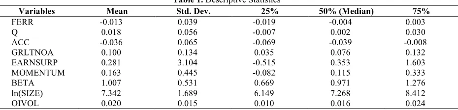
Table 1 presents the descriptive statistics for main variables. Analysts’ earnings forecasts errors (FERR) show a negative mean (-0.013), indicating that sell-side analysts are optimistically biased on average. The mean of Q-score is around zero (0.018) as expected.3 Accruals (ACC) are on average negative(mean : -0.036), while the growth in long-term net operating assets (GRLTNOA), quarterly earnings surprises (EARNSURP), and past stock returns (MOMENTUM) are on average positive (0.100, 0.281, 0.163, respectively). The distributions of these variables as well as the other variables are generally consistent with prior literature.
Table 1 presents the distributions of main variables used in this study. FERR is one-year-ahead analysts’ earnings forecasts errors, measured as one-year-ahead actual earnings per share minus analysts’ one-year-ahead median consensus forecasted earnings per share, scaled by stock price as of April. Q is the Q-score as described in Section 3.1. ACC is accruals, measured as [Δ current asset – Δ current liability – Δ cash + Δ short term debt + Δ
income taxes payable – depreciation expense], scaled by average total assets. GRLTNOA is the growth rates in long term net operating assets, scaled by average total assets. EARNSURP is the standardized unexpected quarterly earnings, which is equal to the current fourth quarter’s actual earnings minus the previous fourth quarter’s actual earnings divided by the standard deviation of the unexpected quarterly earnings over the previous seven quarters. MOMENTUM is the stock returns during the prior twelve months. BETA is the systematic risks estimated by regressing at least thirty but up to sixty prior monthly stock returns against the corresponding market returns. ln(SIZE) is natural logarithm of total assets. OIVOL is the standard deviation of operating income before depreciation of last five years, scaled by average total assets.
Table 1. Descriptive Statistics
Variables Mean Std. Dev. 25% 50% (Median) 75%
FERR -0.013 0.039 -0.019 -0.004 0.003
Q 0.018 0.056 -0.007 0.002 0.030
ACC -0.036 0.065 -0.069 -0.039 -0.008
GRLTNOA 0.100 0.134 0.035 0.076 0.132
EARNSURP 0.281 3.104 -0.515 0.353 1.603
MOMENTUM 0.163 0.445 -0.082 0.115 0.333
BETA 1.007 0.531 0.669 0.971 1.276
ln(SIZE) 7.342 1.689 6.149 7.268 8.412
OIVOL 0.020 0.015 0.010 0.016 0.024
3 The mean value of Q-score of our sample (0.018) exhibit a considerable difference from that of Penman and Zhang (2002)’s study (0.099). It
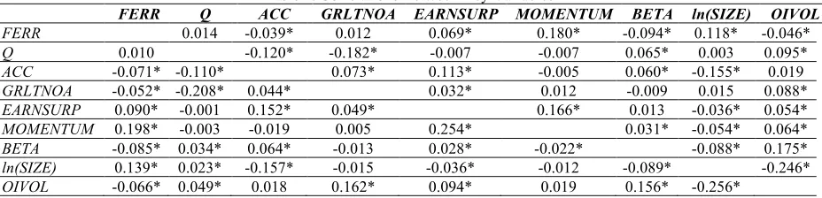
Table 2 reports the Pearson and Spearman correlations between main variables. Analysts’ earnings forecasts errors have a positive correlation with Q-score while it is not significant. And most of variables in the regression equation (1) show the expected signs of correlations with analysts’ earnings forecasts errors. The multicollinearity problem seems not to be so serious because the associations among independent variables stay at low level between -0.20 and 0.20. These uni-variate correlation results should be interpreted with caution because they do not control for differences in other firm characteristics. The multiple regression analysis discussed below controls for such differences.
This table presents Pearson correlation (above diagonal) and Spearman correlation (below diagonal) between analysts’ earnings forecasts errors, Q score and other key variables. Please refer to the note of Table 1 for the definition of the variables.
Table 2. Correlations Between Key Variables
FERR Q ACC GRLTNOA EARNSURP MOMENTUM BETA ln(SIZE) OIVOL
FERR 0.014 -0.039* 0.012 0.069* 0.180* -0.094* 0.118* -0.046*
Q 0.010 -0.120* -0.182* -0.007 -0.007 0.065* 0.003 0.095* ACC -0.071* -0.110* 0.073* 0.113* -0.005 0.060* -0.155* 0.019
GRLTNOA -0.052* -0.208* 0.044* 0.032* 0.012 -0.009 0.015 0.088*
EARNSURP 0.090* -0.001 0.152* 0.049* 0.166* 0.013 -0.036* 0.054*
MOMENTUM 0.198* -0.003 -0.019 0.005 0.254* 0.031* -0.054* 0.064*
BETA -0.085* 0.034* 0.064* -0.013 0.028* -0.022* -0.088* 0.175*
ln(SIZE) 0.139* 0.023* -0.157* -0.015 -0.036* -0.012 -0.089* -0.246*
OIVOL -0.066* 0.049* 0.018 0.162* 0.094* 0.019 0.156* -0.256*
Note: * denotes the significance levels at five percent or less
4. RESULTS
4.1 Replication of Penman and Zhang (2002)
We begin by replicating the results of Penman and Zhang (2002) to examine whether their results still hold in our sample. Using Q-score, the index of current earnings quality, they show that Q-score has a positive relation with the next year’s core return on net operating assets (RNOA), even after controlling for current year’s core RNOA. This result indicates that future earnings will be high (low) with higher (lower) Q-score. They also demonstrate that investors do not fully incorporate this earnings quality into their earnings expectations.
Table 3 presents our replication results. In Panel A, we test whether current year’s Q-score has a predictive power on one-year-ahead core RNOA (CRNOA). We conduct regressions of one-year-ahead core RNOA (CRNOA) on current year’s Q-scores controlling for current year’s core RNOA (CRNOA):
CRNOAt+1 = α0 + α1 CRNOAt + α2 Qt + εt, (5)
Where:
CRNOAt+1(or t) = Core return on net operating assets (RNOA), computed as [operating income after depreciation/
average net operating assets] at time t+1 (or t); and
Qt = Q-score at time t (as described in Section 3.1).
adjustment for serial correlation provided by Kemsley and Nissim (2002)4. As we expect, the estimated coefficient on Q-score is 0.239, with a significant t-statistics of 4.66. This result is consistent with Penman and Zhang (2002), indicating that it is valid to use the Q-score as an earnings quality indicator in our study.
Following Penman and Zhang (2002), we also re-examine whether investors price stocks as if they appreciate the different quality of current earnings implied by the Q-score. Specifically, we conduct regressions of one-year-ahead stock returns on current year’s Q-scores, controlling for frequently used risk proxies as in Penman and Zhang (2002):
RETt+1 = α0 + α1Qt + α2BETAt + α3ln(MV)t + α4ln(B/M)t + α5ln(LEV)t + α6E(+)/Pt + α7(E/P dummy)t + εt, (6)
Where:
RETt+1 = one-Ahead Annual Stock Returns After Q-Scoring (The Year Begins Four Months After Fiscal
Year-End);
Qt = Q-Score (As Described In Section 3.1);
Betat = The Systematic Risks Estimated By Regressing At Least Thirty But Up To Sixty Prior Monthly Stock
Returns Against The Corresponding Market Returns;
Ln(MV)T = The Natural Logarithm Of Market Value Of Equity;
Ln(B/M)T = The Natural Logarithm Of The Book Value Of Equity Divided By The Market Value Of Equity;
Ln(LEV)T = The Natural Logarithm Of The Book Value Of Total Assets Divided By The Book Value Of Equity;
E(+)/Pt = Earnings Per Share Before Extraordinary Items (Reported In I/B/E/S) Divided By Stock Price (Positive
Earnings Only); And
(E/P Dummy)T = Negative Earnings Dummy, 1 If Earnings Are Negative, 0 Otherwise.
Panel A in Table 3 presents the results of cross-sectional year-by-year regression for one-year-ahead core RNOA on Q-score and current core RNOA. CRNOAt(t+1) is core return on net operating assets (RNOA), computed
by [(operating income after depreciation) / average net operating assets] at year t (or t+1). Qt is the Q-score at year t
as described in Section 3.1. Panel B presents the results of cross-sectional year-by-year regression for one-year-ahead stock returns on Q-score and other control variables. RETt+1 is one-year-ahead annual stock returns after
Q-scoring (the year begins four months after fiscal year-end). Qt is Q-score at year t as described in Section 3.1. BETAt
is the systematic risks estimated by regressing at least thirty but up to sixty prior monthly stock returns against the corresponding market returns at year t. ln(MV)t is the natural logarithm of market value of equity at year t. ln(BM)t is
the natural logarithm of the book value of equity divided by the market value of equity at year t. ln(LEV)t is natural
logarithm of the book value of total assets divided by the book value of equity at year t. E(+)/Pt is earnings per share
before extraordinary items (reported in I/B/E/S) divided by stock price, positive earnings only, at year t. (E/P dummy)t is negative earnings dummy, 1 if earnings in year t are negative, 0 otherwise. The coefficients presented in
this table are the means of the annual regressions. The adj. t-stat is the Fama-MacBeth t-statistics (Fama and MacBeth 1973) which is adjusted for autocorrelation as in Kemsley and Nissim (2002). *, ** and *** denotes significance at 0.10, 0.05, 0.01 levels, respectively, using a two-tailed test.
As shown in Panel B, the coefficient of Q-score is significantly positive (coefficient = 0.170, t-stats. = 2.11) after controlling for risk proxies. Therefore, our finding confirms Penman and Zhang’s (2002) result that investors do not fully incorporate the implication of Q-score on future earnings.
4 Since we adopt Fama-MacBeth approach and Q-Score already incorporate the fixed effect, we do not control for year- and
Table 3. Results Of Regression Tests Of The Ability Of Q-Scores To Predict
One-Year-Ahead Core RNOA And Results Of Regression Of One-Year-Ahead Stock Returns On Q-Scores
Panel A : Results Of Regression Tests Of The Ability Of Q-Scores To Predict One-Year-Ahead Core RNOA CRNOAt+1 =α0 + α1 CRNOAt + α2 Qt + εt
Dep. Variable Intercept CRNOAt Qt
CRNOAt+1 0.036*** 0.790*** 0.239***
(adj. t – stat) (6.45) (26.53) (4.66)
Panel B: Results Of Regression Of One-Year-Ahead Stock Returns On Q-Scores RETt+1=α0 + α1 Qt + α2 BETAt + α3ln(MV)t + α4 ln(B/M)t + α5 ln(LEV)t + α6 E(+)/Pt + α7 (E/P dummy)t + εt
Intercept Qt BETAt ln(MV) t ln(B/M) t ln(LEV) t E(+)/Pt (E/P dummy)t
RET t+1 0.162*** 0.170** -0.021 -0.002 0.006 -0.003 0.049 -0.001
(adj. t – stat) (3.66) (2.11) (-1.30) (-0.28) (0.55) (-0.18) (0.49) (-0.05)
4.2 Main Results
In this section, we investigate whether analysts’ earnings forecasts fully reflect the information of current earnings quality indicated by the Q-score. If analysts fully incorporate the different quality of current earnings into their earnings forecasts, then their forecast errors should not be systematically associated with the current year’s Q-score. If not, their forecast errors will be more positive (negative) for firms with higher (lower) Q-Q-score. We first measure analysts’ earnings forecast errors for the subsequent year’s earnings as of April, when is one month after the announcement of the firm’s financial statements. Then, we trace analysts’ earnings forecast errors from April to January of following year to check the degree of effect that Q score has on the analysts’ earnings forecasts errors. We focus on the 10 months from April to January of following year and exclude the data of February and March of following year, because on February and March, a considerable number of I/B/E/S data of analysts’ earnings forecasts are omitted.
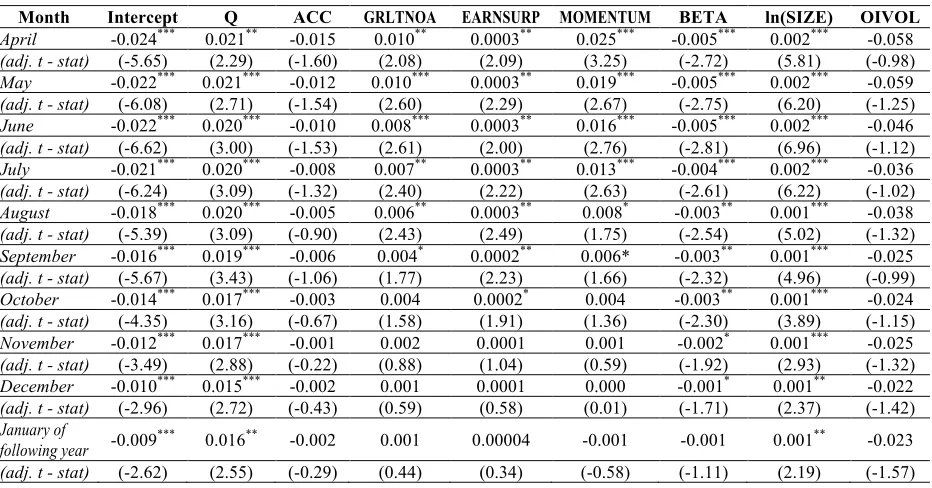
Table 4 provides the result of multivariate regression of analysts’ earnings forecast errors on Q-score. Regressions are performed for each of the 10 months between the April of the year of financial statement announcement and January of following year.
This table presents the results of cross-sectional year-by-year regressions for analysts’ earnings forecasts errors on Q-score and other control variables. Please refer to the note of Table 1 for the definition of the variables except for the following. FERRm,t+1 is one-year-ahead forecasts errors at the end of month m. The coefficients
Table 4. Multivariate Regressions of Analysts’ Earnings Forecast Error on Q-Scores
FERR m,t+1 =α0 + α1 Qt + α2 ACCt + α3 GRLTNOAt + α4 EARNSURPt + α5 MOMENTUMt
+ α6 BETAt + α7 ln(SIZE) t + α8 OIVOLt + εt
Month Intercept Q ACC GRLTNOA EARNSURP MOMENTUM BETA ln(SIZE) OIVOL
April -0.024*** 0.021** -0.015 0.010** 0.0003** 0.025*** -0.005*** 0.002*** -0.058
(adj. t - stat) (-5.65) (2.29) (-1.60) (2.08) (2.09) (3.25) (-2.72) (5.81) (-0.98) May -0.022*** 0.021*** -0.012 0.010*** 0.0003** 0.019*** -0.005*** 0.002*** -0.059
(adj. t - stat) (-6.08) (2.71) (-1.54) (2.60) (2.29) (2.67) (-2.75) (6.20) (-1.25) June -0.022*** 0.020*** -0.010 0.008*** 0.0003** 0.016*** -0.005*** 0.002*** -0.046 (adj. t - stat) (-6.62) (3.00) (-1.53) (2.61) (2.00) (2.76) (-2.81) (6.96) (-1.12) July -0.021*** 0.020*** -0.008 0.007** 0.0003** 0.013*** -0.004*** 0.002*** -0.036
(adj. t - stat) (-6.24) (3.09) (-1.32) (2.40) (2.22) (2.63) (-2.61) (6.22) (-1.02) August -0.018*** 0.020*** -0.005 0.006** 0.0003** 0.008* -0.003** 0.001*** -0.038
(adj. t - stat) (-5.39) (3.09) (-0.90) (2.43) (2.49) (1.75) (-2.54) (5.02) (-1.32) September -0.016*** 0.019*** -0.006 0.004* 0.0002** 0.006* -0.003** 0.001*** -0.025 (adj. t - stat) (-5.67) (3.43) (-1.06) (1.77) (2.23) (1.66) (-2.32) (4.96) (-0.99)
October -0.014*** 0.017*** -0.003 0.004 0.0002* 0.004 -0.003** 0.001*** -0.024
(adj. t - stat) (-4.35) (3.16) (-0.67) (1.58) (1.91) (1.36) (-2.30) (3.89) (-1.15)
November -0.012*** 0.017*** -0.001 0.002 0.0001 0.001 -0.002* 0.001*** -0.025
(adj. t - stat) (-3.49) (2.88) (-0.22) (0.88) (1.04) (0.59) (-1.92) (2.93) (-1.32)
December -0.010*** 0.015*** -0.002 0.001 0.0001 0.000 -0.001* 0.001** -0.022
(adj. t - stat) (-2.96) (2.72) (-0.43) (0.59) (0.58) (0.01) (-1.71) (2.37) (-1.42) January of
following year -0.009*** 0.016** -0.002 0.001 0.00004 -0.001 -0.001 0.001** -0.023 (adj. t - stat) (-2.62) (2.55) (-0.29) (0.44) (0.34) (-0.58) (-1.11) (2.19) (-1.57)
The estimated coefficient of Q-score is significantly positive (Coefficient = 0.021, t-stats. = 2.29) in April (the first month), demonstrating that analysts do not appreciate fully the varying quality of current earnings when they make their initial earnings forecasts. In other words, this result indicates that analysts initially underestimate (overestimate) one-year-ahead earnings when Q-score is relatively high (low). This association remains significant until it comes to January of following year, but the magnitude of coefficients declines from 0.021 to 0.016 as of January of following year (the last month) as illustrated in Figure 1.
The Journal of Applied Business Research – March/April 2015 Volume 31, Number 2
Figure 1. Regression Coefficients Of Q Scores On Analysts’ Earnings Forecasts Errors Across Following Months
We illustrate our result more graphically in Figure 2. Figure 2 depicts the movements of mean analysts’ earnings forecast errors for the one-year-ahead earnings as time goes. More specifically, the mean forecast errors are calculated for portfolios comprised of firm-years in the highest decile of Q-scores (High-Q group) and lowest decile of Q-scores (Low-Q group). The graphs of High-Q group and Low-Q group are depicted as dotted line and solid line, respectively. Also, Figure 2 plots the sample mean forecast errors (thick line) as a benchmark. These three lines are depicted over the 10 months (horizontal axis) following the announcement of financial statements. The left vertical axis lists the mean of analysts’ earnings forecast errors, defined as actual earnings less forecasted earnings, all scaled by the stock price at the end of April. In addition, the right vertical axis lists the difference of forecast errors between High-Q group and Low-Q group, and such differences over the 10 months are described by histograms.
Figure 2 presents analysts’ earnings forecasts errors for the highest and the lowest deciles of portfolios based on Q-scores during the 10 months following financial statement announcement. We defined the highest 10% Q-score portfolios as High-Q group and the lowest 10% Q-score portfolios as Low-Q group. Dotted line indicates High-Q group. Solid line indicates Low-Q group. Thick line indicates the sample mean forecast errors. Histogram is the difference of forecast errors between High-Q group and Low-Q group. Horizontal axis is months. Left vertical axis is the forecast errors, defined as actual earnings less forecasted earnings all scaled by the stock price at the end of April. Right vertical axis is the difference of forecast errors between High-Q group and Low-Q group.
(Months)
0.000 0.005 0.010 0.015 0.020 0.025
Figure 2. Analysts’ Earnings Forecasts Errors For Highest And Lowest Deciles
Of Portfolios Based On Q-Scores During The 10 Months Following Financial Statement Announcement
As depicted by Figure 2, analysts’ earnings forecast errors for the High-Q group are consistently higher than the sample average at all points of time, while the forecast errors of Low-Q group are consistently lower. In addition, as depicted by the histograms, the extent of the differences between High-Q and Low-Q group is the largest in the first month, and gradually decreases as the month progresses. This pattern, consistent with our expectation, implies that analysts do not initially appreciate the future earnings implications of the quality of current earnings indicated by the Q-score. However, analysts increasingly realize the implications of current earnings quality for subsequent year earnings as the month progresses. This may arise from the gradual release of additional earnings-relevant information that is available from subsequent quarterly earnings announcements.
Taken together, our results indicate that analysts do not incorporate fully the joint effect of accounting conservatism and changes in real investment on the quality of current earnings but they gradually correct their forecast errors during the subsequent months, as the future earnings become more predictable due to additional earnings-relevant information.
4.3 Additional Tests
There may be a concern that Q-score and accruals may capture a similar aspect of earnings quality related with the growth of real investment. That is, it might be possible that our main results were driven by the well-known accrual anomaly which was subsumed by Q-score in our sample. However, we believe that accruals anomaly (Sloan 1996) and investors’ mispricing of earnings quality captured by Q-score (Penman and Zhang 2002) are discriminated as follows.
While accruals capture a piece of information about overall fundamental investment (Zhang 2007), Q-score represents the effect of temporary change of real investment under continuous application of accounting conservatism on earnings quality (Penman and Zhang 2002). For example, Fairfield et al. (2001) interpret accruals as the growth in short-term net operating assets and show that investors overreact to accruals as well as the growth of long-term net operating assets. Although this effect may be partially attributed to accounting conservatism (i.e., new investment, rapid depreciation, and decreased subsequent earnings), the accrual anomaly may be interpreted mainly as investors’ overreaction to overall growth of investment. However, Penman and Zhang (2002) build up
Q-0 0.004 0.008 0.012 0.016
-0.02 -0.015 -0.01 -0.005 0
4 5 6 7 8 9 10 11 12 1
Average (Left Axis)
High-Q Group (Left Axis)
Low-Q Group (Left Axis)
(Means of Forecast Errors)(Months)
High-Q Group - Low-Q Group (Right Axis)
score to capture the effect of a temporary change of “hidden reserve”, which is largely affected by conservative accounting, relative to the growth of net operating assets on earnings quality. That is, Q-score captures the temporary growth of “hidden reserve” after controlling for the overall growth of investment. Thus, while accruals capture a piece of information regarding the overall fundamental investment, Q-score focuses on a part of investment, which is treated as expenses under conservative accounting, relative to the overall growth of investment. Based on this reasoning, Penman and Zhang (2002) also argue that Q-score provides incremental information beyond accruals on the effect of growth of real investment on earnings quality.
To address this concern, however, we re-conduct the regression analysis by including either only Q-score or accruals to isolate the effect of each variable on analysts’ earnings forecasts errors. Untabulated results indicate that, when only accruals are included in the regression, the majority of their coefficients are statistically insignificant except the coefficients during the first three months. Furthermore, when only Q-score is included in the regression, the coefficients of Q-score are all significant from April up to January of following year. In addition, we examine the variations of analysts’ earnings forecasts errors across portfolios based on either Q-score or level of accruals. Untabulated results show that the differences between analysts’ earnings forecasts errors of the highest and lowest Q-score portfolios are all statistically significant from April to January of following year, while they are all insignificant for the portfolios based on the level of accruals. Lastly, we rerun the regression equation (6) to identify which of Q-score or accruals dominates the other one in predicting future stock returns. Untabulated results indicate that the independent effect of Q-score on future stock returns is still significant after controlling for accruals.
Taken together, these additional analyses suggest that our main results are not driven by the accrual anomaly which might be subsumed by the Q-score in our sample.
5. CONCLUSION
This study examines whether sell-side analysts’ earnings forecasts fully incorporate the joint effect of accounting conservatism and changes in real investment on future earnings when they forecast future earnings. More specifically, we examine the association between analysts’ earnings forecast errors and the index (i.e. Q-score) of earnings quality. We find a significant association between analysts’ earnings forecasts errors and the index of earnings quality. This result indicates that sell-side analysts do not fully incorporate the quality of current earnings affected by the joint effect of accounting conservatism and changes in real investment on future earnings when they forecast future earnings. This result implies that investors cannot fully incorporate such information simply by using analysts’ earnings forecasts as their benchmark for earnings expectations. This study contributes to the growing body of evidence relating to the efficiency of analysts’ earnings forecast. In addition, our study may promote investors’ assessment of the usefulness or limitation of analysts’ earnings forecasts when they make their earnings expectations.
Notwithstanding a clear contribution of our study, our findings should be interpreted with the following caveats. First, since our analyses require the data of analysts’ earnings forecasts, our sample may be biased toward some types of firms, such as large firms. Accordingly, we admit that our results would not necessarily be generalized to a broader set of firms. We believe, however, that there is no ex-ante expectation that this potential sample selection bias due to the data availability drives our main results. Second, individual firms may have unique firm-specific factors, which affect the analysts’ earnings forecasts errors but are not captured by our control variables. Thus, we cannot fully rule out the possibility that our main empirical results may be driven by omitted variables that we have not controlled for. Lastly, in this study, we examine only the average bias of analysts’ earnings forecasts in incorporating the effects of interaction between accounting conservatism and changes in real investment on the quality of current earnings. However, future research needs to examine the determinants of the cross-sectional variation of association between analysts’ earnings forecasts errors and Q-score, such as information environments, to fully understand the systematic bias of analysts’ earnings forecasts in incorporating such an effect.
ACKNOWLEDGEMENTS
REFERENCES
Abarbanell, J. 1991. “Do analysts’ earnings forecasts incorporate information in prior stock price changes?” Journal of Accounting and Economics 14: 147-165.
Abarbanell, J., and V. Bernard. 1992. “Tests of analysts’ overreaction/underreaction to earnings information as an explanation for anomalous stock price behavior.” Journal of Finance 47 (3): 1181-1207.
Abarbanell, J., and B. Bushee. 1997. “Fundamental analysis, future earnings and stock prices.” Journal of Accounting Research 35 (1): 1-24.
Ali, A., L. Hwang, and M. Trombley. 2003. “Residual-income-based valuation predicts future stock returns: evidence on mispricing vs. risk explanations.” The Accounting Review 78 (2): 377-396.
Beaver, W., and E. Engel. 1996. “Discretionary behavior with respect to allowances for loan losses and the behavior of security prices.” Journal of Accounting and Economics 22: 177-206.
Bradshaw, M., S. Richardson, and R. Sloan. 2001. “Do analysts and auditors use information in accruals?” Journal of Accounting Research 39 (1): 45-74.
Choi, W., T. Kang, Y. Lee, and Y. Yoo. 2008. “A comparison of investors’ and analysts’ efficiency in incorporating accounting information.” Working Paper, Columbia University, Oklahoma State University, and Korea University.
Collins, D., and P. Hribar. 2000. “Earnings-based and accrual-based market anomalies: one effect or two?” Journal of Accounting and Economics 29: 101-123.
Das, S., C. Levine, and K. Sivaramakrishnan. 1998. “Earnings predictability and bias in analysts' earnings forecasts.” The Accounting Review 73 (2): 277-294.
Dechow, M., R. Sloan, and P. Sweeney. 1996. “Causes and consequences of earnings manipulation: An analysis of firms subject to enforcement actions by the SEC.” Contemporary Accounting Research 13 (1): 1-36. Easterwood, J., and S. Nutt. 1999. “Inefficiency in analysts' earnings forecasts: Systematic misreaction or systematic
optimism?” Journal of Finance 54 (5): 1777-1797.
Elgers, P., M. Lo, and R. Pfeiffer. 2003. “Analysts’ vs. investors’ weightings of accruals in forecasting annual earnings.” Journal of Accounting and Public Policy 22: 255-280.
Fama, E., and J. MacBeth. 1973. “Risk, return and equilibrium: Empirical test.” Journal of Political Economy 81: 607-636.
Frankel, R., and C. Lee. 1998. “Accounting valuation, market expectation and cross-sectional stock returns.” Journal of Accounting and Economics 25: 283-319.
Gleason, C., and C. Lee. 2003. “Analyst forecast revisions and market price discovery.” The Accounting Review 78 (1): 193–225.
Gunny, K. 2005. “What are the consequences of real earnings management?” Working Paper, University of California, Berkeley.
Healy, P. 1985. “The effect of bonus schemes on accounting decisions.” Journal of Accounting and Economics 7: 85-107.
Kang, T., and Y. Yoo. 2007. “A comparison of analysts’ and investors’ biases in interpreting accruals: A valuation approach.” Journal of Accounting, Auditing & Finance 22 (3): 383-422.
Kemsley, D., and D. Nissim. 2002. “Valuation of the debt tax shield.” The Journal of Finance 57 (5): 2045-2073. Lee, C., J. Myers, and B. Swaminathan. 1999. “What is the intrinsic value of the Dow?” Journal of Finance 54 (5):
1693-1741.
Lim, T. 2001. “Rationality and analysts' forecast bias.” Journal of Finance 56 (1): 369-385.
Liu, J. 2003. “Market and analyst reactions to earnings news: an efficiency comparison.” Working paper, UCLA. Louis, H., T. Lys, and A. Sun. 2008. “Conservatism and analyst earnings forecast bias.” Working Paper,
Pennsylvania State University.
Mendenhall, R. 1991. “Evidence on the possible underweighting of earnings-related information.” Journal of Accounting Research 29 (1): 170-179.
Mensah, Y., X. Song, and S. Ho. 2004. “The effect of conservatism on analysts’ annual earnings forecast accuracy and dispersion.” Journal of Accounting, Auditing & Finance 19 (2): 159–183.
Moehrle, S. 2002. “Do firms use restructuring charge reversals to meet earnings targets?” The Accounting Review 77 (2): 397-413.
Penman, S., and X. Zhang. 2002. “Accounting conservatism, the quality of earnings and stock returns.” The Accounting Review 77 (2): 237-264.
Pincus, M., S. Rajgopal, and M. Venkatachalam. 2007. “The accrual anomaly: International evidence.” The Accounting Review 82 (1): 169–203.
Richardson, S., R. Sloan, M. Soliman, and I. Tuna. 2005. “Accrual reliability, earnings persistence and stock prices.” Journal of Accounting and Economics 39 (3): 437-485.
Sloan, R. 1996. “Do stock prices fully reflect information in accruals and cash flows about future earnings?” The Accounting Review 71 (3): 289-315.
Stickel, S. 1991. “Common stock returns surrounding earnings forecast revisions: More puzzling evidence.” The Accounting Review 66 (2): 402-416.
Stober, T. 1992. “Summary financial statement measures and analysts’ forecasts of earnings.” Journal of Accounting and Economics 15: 347-372.
Thomas, J., and H. Zhang. 2002. “Inventory changes and future returns.” Review of Accounting Studies 7: 163–187. Xie, H. 2001. “The mispricing of abnormal accruals.” The Accounting Review 76 (3): 357-373.