Microwave radiometer to retrieve temperature proﬁles from the surface to the stratopause

(1)

www.atmos-meas-tech.net/6/2477/2013/ doi:10.5194/amt-6-2477-2013

Atmospheric

Measurement

Techniques

Microwave radiometer to retrieve temperature profiles from the

surface to the stratopause

O. Stähli1, A. Murk1, N. Kämpfer1,2, C. Mätzler1,2, and P. Eriksson3 1_{Institute of Applied Physics, University of Bern, Bern, Switzerland}

2_{Oeschger Centre for Climate Change Research, University of Bern, Bern, Switzerland}

3_{Department of Earth and Space Sciences, Chalmers University of Technology, Göteborg, Sweden}

Correspondence to: O. Stähli ([email protected])

Received: 6 March 2013 – Published in Atmos. Meas. Tech. Discuss.: 21 March 2013 Revised: 29 July 2013 – Accepted: 7 August 2013 – Published: 25 September 2013

Abstract. TEMPERA (TEMPERature RAdiometer) is a new ground-based radiometer which measures in a frequency range from 51–57 GHz radiation emitted by the atmosphere. With this instrument it is possible to measure temperature profiles from ground to about 50 km. This is the first ground-based instrument with the capability to retrieve temperature profiles simultaneously for the troposphere and stratosphere. The measurement is done with a filterbank in combination with a digital fast Fourier transform spectrometer. A hot load and a noise diode are used as stable calibration sources. The optics consist of an off-axis parabolic mirror to collect the sky radiation. Due to the Zeeman effect on the emission lines used, the maximum height for the temperature retrieval is about 50 km. The effect is apparent in the measured spec-tra. The performance of TEMPERA is validated by compar-ison with nearby radiosonde and satellite data from the Mi-crowave Limb Sounder on the Aura satellite. In this paper we present the design and measurement method of the in-strument followed by a description of the retrieval method, together with a validation of TEMPERA data over its first year, 2012.

1 Introduction

Temperature is a key parameter for dynamical, chemical and radiative processes in the atmosphere. There exist several techniques to measure atmospheric temperature profiles like radiosonde (e.g. Luers, 1997; Ruffieux and Joss, 2003), FTIR (Fourier transform infrared, e.g. Smith et al., 1999; Feltz et al., 2003), lidar (e.g. Evans et al., 1997; Alpers et al.,

2004), GPS occultation (e.g. Wickert et al., 2001; Hajj et al., 2002) or satellite and ground-based microwave radiometers (for examples see below). The advantage of ground-based radiometry is the high time resolution at a fixed location that allows for observing local atmospheric dynamics over a long time period. Furthermore, in the near future there might be a lack of satellites which are measuring middle atmospheric profiles of trace gases and temperature. Therefore ground-based radiometry is important to continuously observe the atmosphere.

In the troposphere the atmospheric temperature is im-portant for weather fore- and now-casting. Ground-based microwave radiometers for tropospheric temperature pro-files are well established and exist in different configu-rations. Examples are MICCY (microwave radiometer for cloud cartography) (Crewell et al., 2001), RPG-HATPRO (Radiometer Physics GmbH-Humidity and Temperature Pro-filer) (Rose et al., 2005), Radiometrics MP-3000A (Ware et al., 2003) and ASMUWARA (All-Sky MUlti WAvelength RAdiometer) (Martin et al., 2006).

In the stratosphere temperature can influence chemical processes, and the vertical temperature distribution is im-portant for atmospheric studies to investigate, for example, ozone or water vapor. The middle atmospheric temperature profile also can be affected by dynamical processes such as during sudden stratospheric warming (SSW, e.g. Scherhag, 1952; Flury et al., 2009; Scheiben et al., 2012) events when the temperature in the stratosphere can change by several tens of degrees within a very short time. Therefore it is necessary to obtain temperature profiles with a good temporal and spa-tial resolution. At present, data of stratospheric temperature

(2)

30 dB

R Q L

I 30 dB

5.40 GHz

BW: 0.25 GHz

Detector u1

3.85 GHz Detector

BW: 0.25 GHz

u2

u3

u4 7.00 GHz

BW: 1.00 GHz

Detector

BW: 0.25 GHz

Detector 2.25 GHz

6 1

LO 49−50 GHz

Multiplier (6x) Active Freq. 22 dB

8.50 GHz

BW: 1.20 GHz

50−58 GHz Mixer

20 dB

35 dB 30 dB

Attenuator

diode noise source

Synthesizer 2.8−3.8 GHz IQ Mixer < 4.3 GHz < 0.48 GHz

< 0.48 GHz Sky (30−70°)

10 dB FFT BACK−END

Frontend

Filterbank

Synthesizer 8−8.5 GHz

Ambient load (zenith: 0°)

> 2.3 GHz

digital fft spectrometer

power divider 2−8 GHz

Fig. 1. TEMPERA block diagram.

profiles are mostly obtained by remote sensing methods us-ing radiometers on satellites (e.g. MLS instrument on the Aura satellite as described in Waters et al. (2006), AMSU-A instrument on the AMSU-Aqua satellite as described in AMSU-Aumann et al. (2003) and SABER instrument on the TIMED satellite as described in Remsberg et al. (2003)).

The possibility of ground-based measurements of strato-spheric thermal emission from high-rotational, magnetic dipole transitions of molecular oxygen around 53 GHz was first shown in Waters (1973). It is interesting to note that no realization of a ground-based stratospheric temperature ra-diometer was reported in the literature for several decades. A recent realization of such an instrument was described by Shvetsov et al. (2010).

In this paper we describe the construction, calibration and utilization of a new ground-based TEMPERature RAdiome-ter, called TEMPERA, that is able to monitor temperature structures from ground to the upper stratosphere.

In the following section of this paper we present the mea-surement method and the instrumental set-up of TEMPERA. In the third section we describe the temperature retrieval. In the fourth section a validation of the TEMPERA data and comparison with radiosonde and satellite data is presented.

2 Measurement method and instrument description

2.1 Measurement method

TEMPERA measures thermal radiation from 51–57 GHz in the oxygen-emission region of the microwave spectrum. Oxygen is a well-mixed gas whose fractional concentration is independent of altitude below approx. 80 km. Therefore the radiation contains information primarily on atmospheric temperature.

For tropospheric temperature profiles we measure with a filterbank at 12 frequencies from 51–57 GHz on the wing of the 60 GHz oxygen emission complex. In addition, with a digital fast Fourier transform (FFT) spectrometer, we get in-formation on the temperature profile in the stratosphere by measuring two pressure-broadened emission lines centered at 52.5424 and 53.0669 GHz.

A ground-based microwave radiometer measures a super-position of emission and absorption of radiation at different altitudes. The intensityI can be described with the radiative transfer equation:

I (ν,0)=I0e−τ (ν,s0)₊ s0

Z

0

B(ν, T (s))e−τ (ν,s)α(ν, s)ds, (1)

(3)

Fig. 2. TEMPERA with its main components, the frontend and

the parabolic mirror. TEMPERA is 1.1 m wide. The instrument is placed inside in a thermally controlled lab in front of a blue styro-foam window through which the atmosphere is observed.

coefficient both along the integration paths.B(ν, T )is the Planck function:

B(ν, T )=2hν

3 c2

1 ekThν−1

, (2)

where h is the Planck’s constant, k is the Boltzmann’s constant andcis the speed of light.

The opacity or optical depthτ is defined as

τ (ν, s)= s

Z

0

α(ν, s0)ds0. (3)

In microwave radiometry the measured intensity of radia-tion is often expressed as brightness temperatureTB accord-ing to the Rayleigh–Jeans approximation (valid for the case hνkT) of Planck’s law:

TB(ν,0)=λ

2

2kI (ν,0), (4)

whereλis the wavelength.

The measured spectrum TB(ν,0) is used to retrieve the temperature profile, as described in Sect. 3.1.

2.2 Instrumental description

TEMPERA is a heterodyne receiver covering a frequency range of 51–57 GHz. Figures 1 and 2 give an overview of the instrument. Our instrument consists of three parts: the frontend to collect and detect the microwave radiation with two backends, a filterbank and a digital FFT spectrometer for the spectral analysis. The radiation is directed into the corrugated horn antenna using an off-axis parabolic mirror. The antenna beam has a half-power beamwidth (HPBW) of

4◦_{. The signal is then amplified and downconverted to an}

in-termediate frequency for further spectral analysis. A noise diode in combination with an ambient hot load is used for calibration. The hot load has the room temperature of the lab-oratory (around 293 K). The receiver noise temperatureTN is in a range from 475–665 K. An overview of the technical specifications is given in Table 1.

For the tropospheric measurements we use a filterbank (first backend) with 4 channels. However in the end we ac-tually measure at 12 frequencies, which are listed in Table 2, by adjusting the local oscillator (LO) frequency with a syn-thesizer. For every measured zenith angle the LO frequency is changed three times. In this way we uniformly cover the range from 51–57 GHz at positions between the emission lines (see Fig. 3). The lower 9 channels have a bandwidth of 250 MHz and the channels 10–12 have a bandwidth of 1 GHz to enhance the sensitivity in the flat spectral region.

The second backend is used for stratospheric measure-ments and contains a digital FFT spectrometer (Acqiris AC240) for the two emission lines centered at 52.5424 and 53.0669 GHz. The input signal is coupled from the main sig-nal before the filterbank. It passes an IQ-Mixer (Murk et al., 2009) before being fed to the spectrometer. When the LO frequency is changed by the synthesizer in the frontend, the second synthesizer, which is placed in front of the IQ-Mixer, also changes the frequency. With this method we can al-ways measure the same range with the FFT spectrometer. Furthermore, this allows us to measure the tropospheric and stratospheric part at the same time. With the FFT spectrom-eter in combination with the IQ-Mixer, we can measure the two emission lines with a resolution of 30.5 kHz and a band-width of 960 MHz. The receiver noise temperature TN for the receiver–spectrometer combination is around 480 K. In Table 2 a list with all channels and the corresponding fre-quencies, bandwidths and the receiver noise temperatures is given.

An example of a measured spectrum is shown in Fig. 4. The zoomed lines show the influence of the Zeeman effect by the broadened line shape in the center with a kind of a plateau (round line shape around the line center:±1 MHz).

TEMPERA operates from a temperature-stabilized labo-ratory at the ExWi Building of the University of Bern (Bern, Switzerland: 575 m above sea level; 46.95◦N,7.44◦E, view direction in azimuth: southeast (131.5◦)). A styrofoam win-dow allows views of the atmosphere over the zenith angle (za) range from 30◦_{to 70}◦_{. The operation of the instrument}

inside a laboratory has the advantage that the radiometer is protected against adverse weather conditions. The frontend itself has additional temperature stabilization with Peltier el-ements in combination with a ventilation system leading to a stabilization of the frontend plate within±0.2 K.

(4)

Table 1. Specifications of TEMPERA.

Optical system Corrugated horn antenna with parabolic mirror, HPBW = 4◦ Receiver type Uncooled heterodyne receiver, filterbank; digital FFT spectrometer RF frequency range Filterbank: 51–57 GHz, FFT spectrometer: 52.4–53.2 GHz Receiver operation mode Single sideband

Receiver noise temperature 475–665 K

Filterbank 4 filters, bandwidth 250 MHz and 1 GHz

FFT Spectrometer Bandwidth 1 GHz, resolution 30.5 kHz, 32 768 channels

Mixer (FFT-Backend) I/Q

Calibration Hot load, noise diode

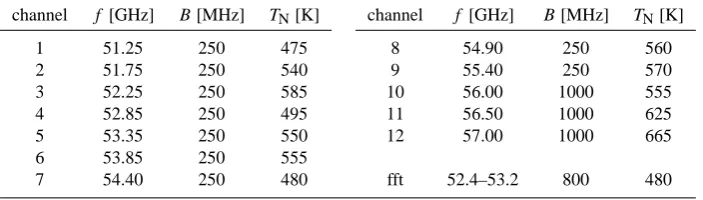
Table 2. Specifications of the 12 tropospheric channels (ch1–ch12) and of the FFT spectrometer (ch_fft) with frequencyf, the bandwidthB and receiver noise temperatureTN.

channel f [GHz] B[MHz] TN[K] channel f [GHz] B[MHz] TN[K]

1 51.25 250 475 8 54.90 250 560

2 51.75 250 540 9 55.40 250 570

3 52.25 250 585 10 56.00 1000 555

4 52.85 250 495 11 56.50 1000 625

5 53.35 250 550 12 57.00 1000 665

6 53.85 250 555

7 54.40 250 480 fft 52.4–53.2 800 480

2.3 Measurement cycle

Measurements are performed in periodic cycles with periods of 60 s. Each cycle starts with hot load calibration in com-bination with a noise diode (see also Sect. 2.4) for 9 s fol-lowed by the atmosphere measurements. They consist of two parts: first a 15 s period at a zenith angle za = 30◦to observe with the FFT spectrometer and simultaneously with the filter-bank, and second, a tipping curve in 3 s periods and angular steps in 5◦up to za = 70◦.

After calibration, the output of each measurement cycle is a set of 108 brightness temperatures of the filterbank at 12 frequencies and at 9 zenith angles and a calibrated spectrum at the two emission lines from the FFT spectrometer consist-ing of 32 768 channels coverconsist-ing the bandwidth of 960 MHz. For the retrieval we use a mean of 15 measurement cy-cles for the troposphere and 120 measurement cycy-cles for the stratosphere, leading to a time resolution of 15 min for tropo-spheric profiles and 120 min for stratotropo-spheric profiles. 2.4 Calibration

Under the assumption of linearity between the antenna tem-peratureTAand the detector-output voltageVTA, as well as

the assumption of a perfect antenna that the brightness tem-peratureTB is equal to TA, the following relation is valid:

TB=TA=VTA

g −TN, (5)

whereg is the effective gain factor and TN is the receiver noise temperature.

The calibration parametersgandTNare obtained from the known radiation of an ambient hot load in combination with a noise diode.

To calibrate the noise diode we use a hot and a cold load. The cold load is a microwave absorber dipped in liquid ni-trogen. Both loads are pyramidal microwave absorbers. With this calibration the so-called excess-noise diode temperature TNDis determined:

TND=(TH−TC)·VHND−VH

VH−VC

, (6)

whereTH is the physical temperature of the hot load,TCis the physical temperature of the cold load (around 77 K at an altitude of 575 m, depending on pressure),V is the detector-output voltage, index H means hot load, HND means hot load with the noise diode switched on, and C means cold load.

The excess-noise diode temperatureTNDis in a range from 40–75 K depending on the frequency.

WithTNDwe can finally calculategandTN: g=VHND−VH

TND (7)

TN=

VH·(TH+TND)−VHND·TH

VHND−VH (8)

(5)

51 52 53 54 55 56 57 100

120 140 160 180 200 220 240 260 280

za=30°

za=50°

za=70°

ch1 ch2

ch3 ch4

ch5

ch6 ch7 ch8 ch9ch10 ch12 ch11 TEMPERA: Spectra Simulation (Qpack2: Summer)

Frequency [GHz]

Brightness Temperature [K]

52.3 52.4 52.5 52.6 52.7 52.8 52.9 53 53.1 53.2 53.3 150

160 170 180 190 200 210 220 230 240 250 260 270

za=30°

za=50°

za=70°

ch_fft

TEMPERA: Spectra Simulation (Qpack2: Summer)

Frequency [GHz]

Fig. 3.Left panel: TEMPERA Spectrum from 51-57 GHz simulated with Qpack2/ARTS2 during summer

for zenith angles at 30◦, 50◦and 70◦. The grey bars indicate the 12 channels (ch1-ch12) of the filterbank.

Right panel: Spectrum from 52-53 GHz simulated with Qpack2/ARTS2 during summer for zenith angles

of 30◦, 50◦and 70◦. The grey bar indicates the available bandwidth of the FFT spectrometer (ch fft).

24

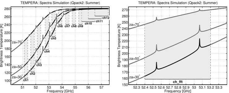
Fig. 3. Left panel: TEMPERA spectrum from 51–57 GHz simulated with Qpack2/ARTS2 during summer for zenith angles at 30, 50 and 70◦.

The grey bars indicate the 12 channels (ch1–ch12) of the filterbank. Right panel: spectrum from 52–53 GHz simulated with Qpack2/ARTS2 during summer for zenith angles of 30, 50 and 70◦; the grey bar here indicates the available bandwidth of the FFT spectrometer (ch_fft).

52.4 52.5 52.6 52.7 52.8 52.9 53 53.1 53.2

155 160 165 170 175 180 185 190 195 200 205

TEMPERA: 2012−01−16, Integration: 09:00−13:00

Frequency [GHz]

52.5224 52.5324 52.5424 52.5524 52.5624 158

160 162 164 166 168 170 172

174TEMPERA: 2012−01−16, Integration: 09:00−13:00

Frequency [GHz]

53.0469 53.0569 53.0669 53.0769 53.0869 188

190 192 194 196 198 200 202 204 206 208

TEMPERA: 2012−01−16, Integration: 09:00−13:00

Frequency [GHz]

Fig. 4.

Spectrum of brightness temperatures measured with TEMPERA on January 16, 2012 from

9h00-13h00 (UT). Upper panel: The whole FFT spectrum, with all channels from 52.4 to 53.2 GHz. The

gap in the middle is due to effects of the filters. Lower panels: Zoomed spectra around the first line at

52.5424 GHz and the second line at 53.0669 GHz.

25

Fig. 4. Spectrum of brightness temperatures measured with

TEM-PERA on 16 January 2012 from 09:00–13:00 (UT). Upper panel: The whole FFT spectrum, with all channels from 52.4 to 53.2 GHz. The gap in the middle is due to effects of the filters. Lower pan-els: zoomed spectra around the first line at 52.5424 GHz and the second line at 53.0669 GHz.

10−4 10−3 10−2 10−1 100

1 2 3 4 5 6 7 8 9 10

Absorption Coefficient [1/km]

Altitude [km]

RS Payerne (ROS98), 2009.1.19 / 23h (UT)

51 GHz→

52.5 GHz→

54 GHz→

55.5 GHz→

57 GHz→

O 2 wv lw N

2

Fig. 5. Absorption Coefficient versus altitude for oxygen (O2),

wa-ter vapor (wv), liquid wawa-ter (lw) and nitrogen (N2) at 51, 52.5, 54,

55.5 and 57 GHz calculated with radiosonde data from Payerne on 19 January 2009 (IWV = 13.11 mm, ILW = 0.19 mm). Calculations made with the Rosenkranz (1998) model.

3 Temperature retrieval

3.1 Retrieval

Our temperature retrieval is based on the optimal estimation method (OEM) (Rodgers, 2000). The forward model F, as expressed by Eqs. (1) and (4), is used to simulate our mea-sured brightness temperature. Here we express it in the fol-lowing equation:

y=F (x,b)+ (9)

(6)

Fig. 6. Temperature profiles derived from TEMPERA from ground

to 50 km from 1 January to 13 December 2012. The white lines indicate the region where MR = 0.6.

where the vectoryis the measured spectrum (brightness tem-perature),xis the true temperature profile,bcontains some additional forward model parameters, andis the measure-ment noise. In our caseF is nonlinear. To retrieve the tem-perature profile from the measured brightness temtem-perature, Eq. (9) has to be inverted. This is an ill-posed problem and to obtain an “optimal” solution a statistical constraint is intro-duced. The solution can be defined as the zero of the gradient of the cost functionJ:

J= [y−F (x)]TS−1[y−F (x)]+[x−xa]TS−a1[x−xa], (10) wherexais the a priori temperature profile, Sais the a priori covariance matrix and Sis the observation error-covariance

matrix.

This principle is based on Bayes’ probability theorem. It is assumed that measurement uncertainties (S) and a priori

knowledge (Sa) both follow Gaussian statistics. On the con-dition that the forward model is not strongly nonlinear, the posterior distribution is then also Gaussian. The solution,x,ˆ

is taken as the state with highest probability, which for Gaus-sian statistics is also the expected value of the distribution.

To find the zero of the derivative of the cost functionJ (Eq. 10) we use the Gauss–Newton iterative method, leading to

xi+1=xi+(S−a1+KTiS −1

Ki)−1

h

KT_iS−1(y−F (xi))

−S−_a1(xi−xa)

i

, (11)

wherexi is the retrieved temperature profile at iterationiand

K is the weighting function (K =∂F/∂x).

The radiative transfer calculations are done with the At-mospheric Radiative Transfer Simulator 2 (ARTS2, Eriksson

220 225 230 235 240 245 250 255 260 265 270 275 280 285 290 1

2 3 4 5 6 7 8 9 10

Temperature [K]

Altitude [km]

TEMPERA: 2011−11−14, Timestart: 11:07

Retrieved temperature Apriori temperature RS Payerne ExWi Bern Zimmerwald

51 52 53 54 55 56 57

100 120 140 160 180 200 220 240 260 280

Frequency [GHz]

Measured signal Fitted signal

Fig. 7.

Measurement of November 14, 2011 at 11h07-11h22 (UT) during clear sky (ILW=0 mm). Upper

panel: Retrieved temperature profile (blue line). The a-priori profile is the dashed black line. Comparison

with radiosonde data from Payerne (red line) and with weather station data from Bern (black circle),

Zim-merwald (blue circle). Lower panel: Brightness temperatures of 12 channels measured with TEMPERA

(black) compared with the forward model brightness temperatures (red) corresponding to the retrieval.

27

Fig. 7. Measurement of 14 November 2011 at 11:07–11:22 (UT)

during clear sky (ILW = 0 mm). Upper panel: retrieved temperature profile (blue line). The a priori profile is the dashed black line; com-parison with radiosonde data from Payerne (red line), with weather station data from Bern (black circle), and with Zimmerwald (blue circle). Lower panel: brightness temperatures of 12 channels mea-sured with TEMPERA (black dots) compared with the forward model brightness temperatures (open red dots) corresponding to the retrieval.

et al., 2011). The inversion is treated in Qpack2 (Eriksson et al., 2005).

The retrieval is calculated on a pressure grid. We use the same resolution for the retrieval grid as for the forward model grid. In this paper all data are plotted in geometric height in km for practical reasons. For the conversion from a pressure grid to a kilometer grid we used radiosonde and ECMWF (European Centre for Medium-Range Weather Forecasts) data.

(7)

Table 3. List of used line parameters for O₂. The data are from the PWR93 oxygen absorption model (Rosenkranz, 1993).

Quantum ν S(300 K) b w y v

ID [GHz]

h cm2Hz

i

[ ] h

MHz hPa

i h

10−3 hPa

i h

10−3 hPa

i

29- 52.5424 0.4264×10−16 6.004 0.94 0.7702 0.6526

27- 53.0669 0.8898×10−16 5.224 0.97 0.7348 0.6206

−5 0 5 10 15 20

1 2 3 4 5 6 7 8 9 10

Altitude [km]

10 MR FWHM [km] 100 AVK

0 0.2 0.4 0.6 0.8 1 1.2 1.4 1.6 1.8 2

1 2 3 4 5 6 7 8 9 10

Temperature retrieval error [K]

Altitude [km]

total error observation error smoothing error cal. error Spect. (O₂) H₂O

total sys. error

Fig. 8.

Measurements of November 14, 2011 at 11h07-11h22 (UT) during clear sky (ILW=0 mm). Upper

panel: The averaging kernels (AVK, plotted every 4th) of TEMPERA are shown in this plot together with

the measurement response (MR) and the full-width at half-maximum (FWHM, in km). Lower panel: Error

of the retrieval. The error statistics contain the total error (solid red) consisting of observation error (solid

blue) and smoothing error (solid black). The total systematic error (dotted black) contains the uncertainties

in the calibration (dashed blue), in the oxygen profile (”spectroscopic error”, dashed red) and in the water

vapor profile (dashed black).

28

Fig. 8. Measurements of 14 November 2011 at 11:07–11:22 (UT)

during clear sky (ILW = 0 mm). Upper panel: the averaging kernels (AVK, plotted every 4th) of TEMPERA are shown in this plot to-gether with the measurement response (MR) and the full-width at half-maximum (FWHM, in km). Lower panel: error of the retrieval. The error statistics contain the total error (solid red) consisting of observation error (solid blue) and smoothing error (solid black). The total systematic error (dotted black) contains the uncertainties in the calibration (dashed blue), in the oxygen profile (“spectroscopic er-ror”, dashed red) and in the water vapor profile (dashed black).

220 225 230 235 240 245 250 255 260 265 270 275 280 285 290 1

2 3 4 5 6 7 8 9 10

Temperature [K]

Altitude [km]

Retrieved temperature Apriori temperature RS Payerne ExWi Bern Zimmerwald

53 53.5 54 54.5 55 55.5 56 56.5 57

210 220 230 240 250 260 270 280

Frequency [GHz]

Fig. 9.

Measurement of November 14, 2011 at 22h57-23h12 (UT) during cloudy sky (ILW=0.1 mm).

Upper panel: Temperature profile (blue line) retrieved with TEMPERA. The a-priori profile is the dashed

black line. The retrieved profile is compared with radiosonde data from Payerne (red line) and with

weather station data from Bern (black circle), Zimmerwald (blue circle). Lower panel: Brightness

tem-peratures of 8 channels measured with TEMPERA (black) compared with the forward model brightness

temperatures (red) corresponding to the retrieval.

29

Fig. 9. Measurement of 14 November 2011 at 22:57–23:12 (UT)

during cloudy sky (ILW = 0.1 mm). Upper panel: temperature pro-file (blue line) retrieved with TEMPERA. The a priori propro-file is the dashed black line. The retrieved profile is compared with ra-diosonde data from Payerne (red line), with weather station data from Bern (black circle), and with Zimmerwald (blue circle). Lower panel: brightness temperatures of 8 channels measured with TEM-PERA (black) compared with the forward model brightness temper-atures (red) corresponding to the retrieval.

(8)

Table 4. Estimated uncertainties for the calculations of the

system-atic retrieval errors.

Troposphere: Parameter Uncertainty

Water vapor 10 %

Oxygen (“spectroscopic error”) 1 %

Calibration 0.5 K

Stratosphere: Parameter Uncertainty

Water vapor 10 %

Oxygen (“spectroscopic error”) 1 %

Calibration 1.5 K

of the retrieved temperature profilexˆto a change in the “true” profilex:

A=DyKx=

∂xˆ

∂x, (12)

where Kx=∂F/∂x is the weighting function matrix and

Dy=∂x/∂yˆ is the contribution function.

The rows of A are called the averaging kernels (AVK). Every row describes the sensitivity of the retrieval for a cer-tain height level to a perturbation at other levels. The sum of the AVK is called the measurement response (MR), which describes the contribution of measurement to the retrieved profile at a certain height. The full-width at half-maximum (FWHM) of the AVK is often used as a height resolution of the retrieval.

There exist different methods to compare profiles from a ground-based radiometer with a reference profile from col-located radiosondes and satellites. One possibility is to inter-polate the reference profiles at levels of the radiometer and compare it directly. A second method is to convolve the in-terpolated reference profilexr with the averaging kernel A of the radiometer to take into account the different height resolutions:

ˆ

xr=xa+A(xr−xa), (13) wherexais the a priori profile of the radiometer.

3.2 Forward model parameters

In the radiative transfer calculations we use the model of Rosenkranz and the model of Liebe for the absorption coeffi-cient calculations: Rosenkranz (1998) for H2O, Rosenkranz (1993) for O2and Liebe et al. (1993) for N2. The used line parameters for the oxygen (O2) spectral lines are listed in Table 3.

In the forward model a water-vapor profile with an expo-nential decrease is included. This profile is calculated with the measured surface water vapor density from the ExWi-Weather station (placed next to TEMPERA) and assuming a scale height of 2000 m. Further descriptions can be found in Bleisch et al. (2011). For other species like oxygen (O2) and

−5 0 5 10 15 20

1 2 3 4 5 6 7 8 9 10

Altitude [km]

0 0.2 0.4 0.6 0.8 1 1.2 1.4 1.6 1.8 2

1 2 3 4 5 6 7 8 9 10

Altitude [km]

total error observation error smoothing error cal. error Spect. (O

2)

H

2O

total sys. error

Fig. 10.

Measurement of November 14, 2011 at 22h57-23h12 (UT) during cloudy sky (ILW=0.1 mm).

Upper panel: The averaging kernels (AVK, plotted every 4th) of TEMPERA are shown in this plot together

with the measurements response (MR) and the full-width at half-maximum (FWHM, in km). Lower panel:

Error of the retrieval. The error statistics contain the total error (solid red) consisting of observation error

(solid blue) and smoothing error (solid black). The total systematic error (dotted black) contains the

uncertainties in the calibration (dashed blue), in the oxygen profile (”spectroscopic error”, dashed red)

and in the water vapor profile (dashed black).

30

Fig. 10. Measurement of 14 November 2011 at 22:57–23:12 (UT)

during cloudy sky (ILW = 0.1 mm). Upper panel: the averaging ker-nels (AVK, plotted every 4th) of TEMPERA are shown in this plot together with the measurements response (MR) and the full-width at half-maximum (FWHM, in km). Lower panel: error of the retrieval. The error statistics contain the total error (solid red) consisting of observation error (solid blue) and smoothing error (solid black). The total systematic error (dotted black) contains the uncertainties in the calibration (dashed blue), in the oxygen profile (“spectroscopic er-ror”, dashed red) and in the water vapor profile (dashed black).

nitrogen (N2) we used standard atmospheric profiles for sum-mer and winter, which are incorporated into ARTS2 (mid-dle latitude FASCODE (Fast Atmospheric Signature CODE) (Anderson et al., 1986)).

(9)

260 270 280 290

0.9 km (910 hPa) / Corr−coeff: 0.99

T [K]

260 270 280 290

1.4 km (856 hPa) / Corr−coeff: 0.971

T [K]

260 270 280 290

2.4 km (759 hPa) / Corr−coeff: 0.915

T [K]

250 260 270 280

4.1 km (611 hPa) / Corr−coeff: 0.876

T [K]

Jan 12 Feb 12 Mar 12 Apr 12 May 12 Jun 12 Jul 12 Aug 12 Sep 12 Oct 12 Nov 12 Dec 12

230 240 250

7.8 km (373 hPa) / Corr−coeff: 0.845

#: 644 o TEMPERA x RS PAY −− a priori / Retrieval: v12

T [K]

Fig. 11.Time-series from January, 1 to December, 13 2012 (644 profiles) of tropospheric temperature

pro-files from TEMPERA (blue) compared with radiosonde data from Payerne (red, regridded to TEMPERA

grid) for five different altitude levels. The black dashed line is the a-priori.

31

Fig. 11. Time series from 1 January to 13 December 2012 (644 profiles) of tropospheric temperature profiles from TEMPERA (blue)

compared with radiosonde data from Payerne (red, regridded to TEMPERA grid) for five different altitude levels. The black dashed line is the a priori.

is more or less the same for the 5 frequencies. This is not true for oxygen, which is strongly dependent on frequency. Furthermore, the figure shows that cloud liquid has a sim-ilar absorption coefficient as oxygen in the frequency range from 51 to 53 GHz. On the other hand, during clear sky (inte-grated liquid water, ILW = 0 mm) the main part of the absorp-tion and emission in the atmosphere is from oxygen dominat-ing the contribution from water vapor and nitrogen. Further discussion about temperature retrieval during weather condi-tions with and without clouds will be presented in Sect. 4.2. 3.3 Weighting functions

Accurate and rapid calculations of weighting functions (WFs) are important for obtaining stable and fast inversions. The general approach in ARTS to extract WFs is outlined by Buehler et al. (2005); some improvements have since been added. As part of this study, the analytical expressions used for temperature WFs were expanded to also consider local effects caused by the constraint of hydrostatic equilibrium. These resulting WFs cover all relevant aspects of the mea-surements of concern here, and the extension has drastically improved the calculation speed. See the user guide of ARTS2 (www.sat.ltu.se/arts/docs) for the expressions used and their limitations (e.g. they are not valid for limb sounding).

3.4 Error analysis

The total error of a retrieval consists mainly of the observa-tion error due to the measurement noise and uncertainty as well as the smoothing error caused by the vertical smoothing of the retrieval method. The estimations of the observation covariance matrix (So) and the smoothing covariance matrix (Ss) are shown in the following equations (Rodgers, 2000):

So=DySDTy (14)

Ss=(A−I)Sa(A−I)T (15)

where I is the identity matrix. The total error of the observa-tion and of the vertical smoothing is calculated as the square root of the diagonal elements of the covariance matrix Soand Ss, respectively.

Additionally there exist the systematic errors. We calcu-late the systematic errors by considering the estimated un-certainties in the water vapor profile, in the oxygen profile (“spectroscopic error”) and in the calibration. This is done by a perturbation approach where we change the respective profiles and the calibration within the estimated limits and compare with the standard retrieval. The used estimated val-ues are listed in Table 4. The total systematic error is cal-culated as the square root of the sum of the variances from water vapor, oxygen and calibration.

(10)

−5 −4 −3 −2 −1 0 1 2 3 4 5 1

2 3 4 5 6 7 8 9 10

MR≥0.6 ↓

#: 644 / Retrieval: v12

Altitude [km]

T_TEMPERA−T_{RS Pay} [K]

−5 −4 −3 −2 −1 0 1 2 3 4 5

1 2 3 4 5 6 7 8 9 10

MR≥0.6 ↓

Altitude [km]

T_TEMPERA−T_{RS Pay conv.} [K]

Fig. 12.

Comparison of 644 profiles (January, 1 to December, 13 2012) between TEMPERA and

ra-diosonde data from Payerne over an altitude range from ground (0.575 km) to 10 km. Plotted is the mean

(black line) and plus and minus one standard deviation around the mean (black dashed line) of the

dif-ference between TEMPERA and radiosonde data from Payerne. The horizontal grey line indicates the

region where MR=0.6. Upper panel: TEMPERA compared with unconvolved radiosonde data from

Pay-erne. Lower panel: TEMPERA compared with convolved radiosonde data from Payerne over a altitude

region with MR

≥

0.6.

32

Fig. 12. Comparison of 644 profiles (1 January to 13

Decem-ber 2012) between TEMPERA and radiosonde data from Payerne over an altitude range from ground (0.575 km) to 10 km. Plotted are the mean (black line) and plus and minus one standard devia-tion around the mean (black dashed line) of the differences between TEMPERA and radiosonde data from Payerne. The horizontal dark grey line indicates the region where MR = 0.6. Upper panel: TEM-PERA compared with unconvolved radiosonde data from Payerne. Lower panel: TEMPERA compared with convolved radiosonde data from Payerne over an altitude region with MR≥0.6.

3.5 Tropospheric retrieval

As mentioned before, 12 channels are used (Table 2) to re-trieve tropospheric temperature profiles. Additionally, we use information from 9 zenith angles (30◦to 70◦, every 5◦).

The retrieval software Qpack2 (Eriksson et al., 2005) uses a pressure grid for the retrieval calculations. We use the same resolution for the retrieval grid as for the forward model

0.75 0.775 0.8 0.825 0.85 0.875 0.9 0.925 0.95 0.975 1 1

2 3 4 5 6 7 8 9 10

Altitude [km]

Correlation coefficient MR≥0.6 ↓

Corrcoeff(T

TEMPERA,TRS Pay) Corrcoeff(T

TEMPERA,TRS Pay conv.)

Fig. 13.

Correlation coefficient of the comparison for 644 profiles (January, 1 to December, 13 2012)

between TEMPERA and radiosonde data from Payerne over an altitude range from ground (0.575 km)

to 10 km. The horizontal grey line indicates the region where MR=0.6. Correlation coefficient of the

comparison between TEMPERA and the unconvolved (black line) and convolved (dashed black line,

altitude region with MR

≥

0.6) radiosonde data from Payerne.

33

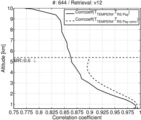
Fig. 13. Correlation coefficient of the comparison of 644 profiles

(1 January to 13 December 2012) between TEMPERA and ra-diosonde data from Payerne over an altitude range from ground (0.575 km) to 10 km. The horizontal dark grey line indicates the region where MR = 0.6. Panel shows correlation coefficient of the comparison between TEMPERA and the unconvolved (black line) and convolved (dashed black line, altitude region with MR≥0.6) radiosonde data is from Payerne.

grid. Our first pressure-grid point is at the surface where our instrument is situated. This pressure value is taken from our weather station at the measurement time. The other grid points are selected in such a way that we have more grid points in the lower troposphere than in the upper troposphere because the measurements contain most information from the lowest layers of the troposphere. Our grid has a resolu-tion of about 100 m from ground to 1 km, about 300 m from 1 to 5 km and about 500 m from 5 to 10 km.

As an a priori temperature profile, monthly mean ra-diosonde data from Payerne (46.82◦N, 6.95◦E; 491 m above sea level and 40 km W of Bern) are used. The data are from 1994 to 2011 and the soundings are twice a day at 11:00 and at 23:00 (UT). For the a priori covariance matrix Sawe use a correlation function decreasing exponentially with a corre-lation length of 3 km. A standard deviation of 2 K at ground, decreasing linearly to 1.5 K at 15 km, is assumed. The obser-vation error is considered in the covariance matrix S as a

(11)

210 220 230 240 250 260 270 280 15

20 25 30 35 40 45 50 55

TEMPERA: 2012−06−15, Time: 12:04−14:04

Temperature [K]

Altitude [km]

Retrieved temperature Apriori temperature RS Payerne MLS

175 180 185 190 195 200 205 210 215 220 225

Brightness Temp. [K]

TEMPERA: 2012−06−15, Time: 12:04−14:04

52.5 52.6 52.7 52.8 52.9 53 53.1 −3

−1.50 1.53

Frequency [GHz]

B. T. [K] Residuals

Fig. 14.

Measurement of June 15, 2012 from 12h04-14h04 (UT) during clear sky (ILW=0 mm).

Up-per panel: TemUp-perature profile (blue line) retrieved with TEMPERA spectrometer measurements. The

a-priori profile is the dashed black line. The retrieved profile is compared with radiosonde data from

Payerne (black line) and with MLS data (red). Lower panel: Brightness temperatures measured with

TEMPERA (black) compared with the forward model brightness temperatures (red) that we received with

the retrieval. Below the residuals are seen. In the forward model

±

1 MHz around the two line centers

we have no frequencies points in the grid, because until now the Zeeman effect has not been incorporated

in Qpack2/ARTS2. In the center of the lines (

±

16 MHz, 1000 channels) we use all channels and on the

wings of the line we use a binning of 3 channels for data reduction.

34

Fig. 14. Measurement of 15 June 2012 from 12:04–14:04 (UT)

dur-ing clear sky (ILW = 0 mm). Upper panel: temperature profile (blue line) retrieved with TEMPERA spectrometer measurements. The a priori profile is the dashed black line. The retrieved profile is com-pared with radiosonde data from Payerne (black line) and with MLS data (red). Lower panel: Brightness temperatures measured with TEMPERA (black) compared with the forward model brightness temperatures (red) that we received with the retrieval. Low in the panel the residuals are seen. In the forward model±1 MHz around the two line centers we have no frequencies points in the grid be-cause until now the Zeeman effect has not been incorporated into Qpack2/ARTS2. In the center of the lines (±16 MHz, 1000 chan-nels) we use all channels and on the wings of the line we use a binning of 3 channels for data reduction.

3.6 Stratospheric retrieval

The stratospheric temperature profile is retrieved from the measurement of the two emission lines, centered at 52.5424 and 53.0669 GHz. We use the two lines at the same time with a bandwidth of 200 MHz around 52.5424 GHz and 160 MHz around 53.0669 GHz. With the digital FFT spectrometer we measure at a zenith angle of 30◦. In Fig. 3 the simulated spec-tra at the three different zenith angles 30, 50 and 70◦can be

−5 0 5 10 15 20

15 20 25 30 35 40 45 50 55

Altitude [km]

TEMPERA: 2012−06−15, Time: 12:04−14:04

0 0.2 0.4 0.6 0.8 1 1.2 1.4 1.6 1.8 2 2.2 2.4 15

20 25 30 35 40 45 50 55

Altitude [km]

TEMPERA: 2012−06−15, Time: 12:04−14:04

total error observation error smoothing error cal. error Spect. (O₂) H₂O

total sys. error

Fig. 15.

Measurement of June 15, 2012 from 12h04-14h04 (UT) during clear sky (ILW=0 mm). Upper

panel: The averaging kernels (AVK, plotted every 7th) of TEMPERA are shown in this plot together with

the measurements response (MR) and the full-width at half-maximum (FWHM, in km). Lower panel:

Error of the retrieval. The error statistics contain the total error (solid red) consisting of observation error

(solid blue) and smoothing error (solid black). The total systematic error (dotted black) contains the

uncertainties in the calibration (dashed blue), in the oxygen profile (”spectroscopic error”, dashed red)

and in the water vapor profile (dashed black).

35

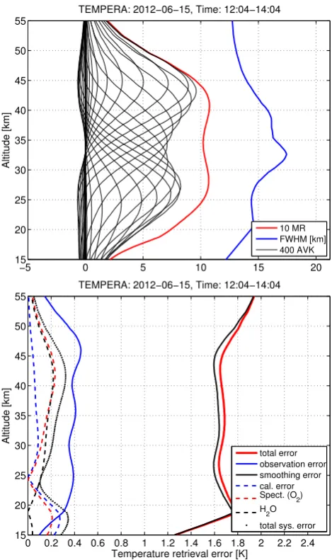
Fig. 15. Measurement of 15 June 2012 from 12:04–14:04 (UT)

dur-ing clear sky (ILW = 0 mm). Upper panel: The averagdur-ing kernels (AVK, plotted every 7th) of TEMPERA are shown in this plot to-gether with the measurements response (MR) and the full-width at half-maximum (FWHM, in km). Lower panel: error of the retrieval. The error statistics contain the total error (solid red) consisting of observation error (solid blue) and smoothing error (solid black). The total systematic error (dotted black) contains the uncertainties in the calibration (dashed blue), in the oxygen profile (“spectroscopic er-ror”, dashed red) and in the water vapor profile (dashed black).

seen. The results show that the intensity of the emission lines is highest at za = 30◦_{. Therefore we decided to measure the}

emission lines at this angle.

During a measurement cycle the integration time with the FFT spectrometer is 15 s. For a temperature profile we in-tegrate the measurement for half an hour because then the noise level is low enough to get good retrievals. This re-quires two hours of measurement time because only one quarter of the measurement time is spent for the digital

(12)

200 210 220

20.1 km (54 hPa) / Corr−coeff: 0.802

T [K]

200 210 220

22.5 km (37 hPa) / Corr−coeff: 0.873

T [K]

200 210 220 230

25 km (25 hPa) / Corr−coeff: 0.89

T [K]

190 200 210 220 230

240 27 km (18 hPa) / Corr−coeff: 0.914

T [K]

Jan 12 Feb 12 Mar 12 Apr 12 May 12 Jun 12 Jul 12 Aug 12 Sep 12 Oct 12 Nov 12 Dec 12

210 220 230 240

29.5 km (12 hPa) / Corr−coeff: 0.916

#: 524 o TEMPERA x RS PAY −− a priori / Retrieval: v2

T [K]

Fig. 16.Timeseries (524 profiles) of stratospheric temperature profiles from TEMPERA (blue) compared

with radiosonde data from Payerne (red, regridded to TEMPERA grid) for five different altitude levels.

The black dashed line is the a-priori.

36

Fig. 16. Time series (524 profiles) of stratospheric temperature profiles from TEMPERA (blue) compared with radiosonde data from Payerne

(red, regridded to TEMPERA grid) for five different altitude levels. The black dashed line is the a priori.

FFT spectrometer. The remaining period of the measurement TEMPERA measures at za = 35–70◦_{with the filterbank only}

(see also Sect. 2.3). For the forward model we use a vertical grid with a resolution of about 350 m. The retrieval grid has the same vertical resolution. Further in the forward model

±1 MHz around the two line centers we have no frequency points in the grid because the Zeeman effect is not yet fully incorporated into Qpack2/ARTS2. In the center of the lines (±16 MHz, 1000 channels) we use all channels, and on the wings of the line we use a binning of 3 channels for data reduction.

As a temperature a priori profile from ground to about 15 km we use the monthly mean of radiosonde data from Payerne from 1994 to 2011. Above, a climatology of the Mi-crowave Limb Sounder (MLS) data (Aura satellite) is used. For the a priori covariance matrix Sa we use a correlation function decreasing exponentially with a correlation length of 3 km. A standard deviation of 2 K is assumed. The obser-vation error (residual) is considered in the covariance matrix S as a diagonal matrix. The residual is the difference

be-tween the integrated spectra and the fit of the spectra. Under regular conditions the observation error is in a range from 0.5 to 1.5 K. Around 52.5424 GHz (first line) the noise is higher than around at 53.0669 GHz (second line), as shown in Fig. 4. We retrieve a temperature profile every 2 h, resulting in 12 profiles per day. To avoid effects due to clouds the strato-spheric retrieval is done for conditions with ILW≤0.1 mm.

4 Temperature profiles: results

4.1 Introduction

Here we present an analysis of temperature retrievals from TEMPERA over almost one year, during the period from 1 January to 13 December 2012. The data consist of 2929 stratospheric profiles and 33 021 tropospheric profiles. The whole data set, covering the height range from ground to 50 km, can be seen in Fig. 6. The merging of the two indepen-dent data sets was done in a way that we use the tropospheric data from ground to 14 km and the stratospheric data from 14 to 50 km. Because of the different time resolutions we had to adapt the stratospheric data to the time axis of the tro-pospheric data. There was an interpolation in time necessary. The white lines indicate the measurement response MR = 0.6. The altitude range with MR≥0.6 is from ground to 5–6 km (troposphere) and from 18 to 48 km (stratosphere). The tro-pospheric data are for all weather conditions, and the strato-spheric data are for conditions with ILW≤0.1 mm to avoid effects due to clouds. The information about clouds (ILW) are from the radiometer TROWARA (TRopospheric WAter vapor RAdiometer) (Mätzler and Morland, 2009), which is installed next to TEMPERA, measuring the radiation from the sky in the same direction at 21, 22 and 31 GHz.

(13)

−10 −8 −6 −4 −2 0 2 4 6 8 10 10

12 14 16 18 20 22 24 26 28

MR_≥0.6 _↑

Altitude [km]

T

TEMPERA−TRS Pay [K]

−10 −8 −6 −4 −2 0 2 4 6 8 10

10 12 14 16 18 20 22 24 26 28

MR_≥0.6 _↑

Altitude [km]

T

TEMPERA−TRS Pay conv. [K]

Fig. 17.

Comparison of 524 profiles (January, 1 to December, 13 2012) between TEMPERA and

ra-diosonde data from Payerne over an altitude range from 10 km to about 29 km. Plotted is the mean (black

line) and plus and minus one standard deviation around the mean (black dashed line) of the difference

be-tween TEMPERA and radiosonde data from Payerne. The horizontal grey line indicates the region where

MR=0.6. Upper panel: TEMPERA compared with unconvolved radiosonde data from Payerne. Lower

panel: TEMPERA compared with convolved radiosonde data from Payerne over a altitude region with

MR

≥

0.6.

37

Fig. 17. Comparison of 524 profiles (1 January to 13

Decem-ber 2012) between TEMPERA and radiosonde data from Payerne over an altitude range from 10 km to about 29 km. Plotted are the mean (black line) and plus and minus one standard deviation around the mean (black dashed line) of the difference between TEM-PERA and radiosonde data from Payerne. The horizontal dark grey line indicates the region where MR = 0.6. Upper panel: TEMPERA compared with unconvolved radiosonde data from Payerne. Lower panel: TEMPERA compared with convolved radiosonde data from Payerne over an altitude region with MR≥0.6.

coefficients of the coincident profiles displayed in this paper have a confidence level above 95 %.

4.2 Tropospheric temperature profiles

4.2.1 Clear sky measurements

Figure 7 shows a typical result of a temperature profile (upper plot) at times without liquid water compared with the profiles

obtained by a nearby radiosonde site and the a priori profile. The corresponding brightness temperatures (lower plot) from 14 November 2011 at 11:00 (UT) are also shown. In this case we use all 12 channels and 9 zenith angles, with a total of 108 measured brightness temperatures.

At this time point an inversion between 1000 m and about 3000 m was present. Nevertheless the retrieved temperature profile from TEMPERA measurements agrees well with the radiosonde profile from Payerne and the weather stations from Bern and Zimmerwald (46.88◦N, 7.47◦E; 905 m above sea level and 10 km S of Bern).

The forward model brightness temperatures, calculated for the retrieved profile, agree well with the measured bright-ness temperatures for all channels. The absolute difference between measured and forward model brightness tempera-tures (residuals) is between 0.05 and 1.2 K. The averaging kernels, the height resolution (FWHM of the averaging ker-nels) and the measurement response are shown in Fig. 8. The height resolution in the first kilometer is about 300 m. From 1 to 10 km the height resolution increases to around 5 km.

The retrieval error, calculated with Eqs. (14) and (15), and the systematic errors are shown in Fig. 8. The retrieval er-ror is less than 0.5 K from ground to 1 km and then increases linearly to 1.5 K at 10 km. It is also seen that the observation error is much smaller than the smoothing error. The total sys-tematic error is between 0.5 and 1.5 K in the altitude range from ground to 10 km.

This example shows that during clear sky we get good results compared with the radiosondes and weather stations from ground up to 7 km with a measurement response higher than 0.6. From 7 to 10 km the measurement response is smaller than 0.6 and therefore more information from the a priori profile is used than from the measurements.

4.2.2 Measurements with cloudy sky

To retrieve temperature profiles during cloudy sky the lowest 4 channels between 51.25–52.85 GHz are not taken into ac-count in the calculations due to the unknown cloud influence shown in Fig. 5. We choose a threshold of ILW = 0.025 mm in order to use only 8 channels. Below this threshold value the retrieval takes into account all 12 channels. At the mo-ment we do not take into account the liquid water (clouds) in the forward model. With this simple but effective method we get reasonable results.

A typical result of a temperature profile from 14 Novem-ber 2011 at 23:00 (UT) with ILW = 0.1 mm is shown in Fig. 9. This measurement contains 8 frequencies (channels 5–12: 53.35–57 GHz) and 9 zenith angles providing 72 mea-sured brightness temperatures (see also Fig. 9). The for-ward model brightness temperatures agree with the mea-sured brightness temperatures, with an absolute difference between measured and forward model brightness tures (residuals) between 0.05 and 1.8 K. Also, the tempera-ture profile from TEMPERA agrees with the radiosonde data

(14)

200 210 220

25 km (25 hPa) / Corr−coeff: 0.92

T [K]

200 210 220 230 240

30.1 km (11 hPa) / Corr−coeff: 0.927

T [K]

210 220 230 240 250

T [K]

220 230 240 250 260 270

280 40.2 km (3 hPa) / Corr−coeff: 0.923

T [K]

Jan 12 Feb 12 Mar 12 Apr 12 May 12 Jun 12 Jul 12 Aug 12 Sep 12 Oct 12 Nov 12 Dec 12 240

250 260 270 280

#: 243 o TEMPERA x MLS −− a priori / Retrieval: v2

T [K]

Fig. 18.Timeseries (243 profiles) of stratospheric temperature profiles from TEMPERA (blue) compared

with MLS data (red, regridded to TEMPERA grid) for five different altitude levels. The black dashed line

is the a-priori.

38

Fig. 18. Time series (243 profiles) of stratospheric temperature profiles from TEMPERA (blue) compared with MLS data (red, regridded to

TEMPERA grid) for five different altitude levels. The black dashed line is the a priori.

from Payerne and the weather stations from Bern and Zim-merwald. The best agreements are in the altitude range from ground to about 2.5 km.

The averaging kernels, the height resolution (FWHM of the averaging kernels) and the measurement response are shown in Fig. 10. The height resolution is similar to reso-lution for clear sky. During cloudy sky the measurement re-sponse is higher than 0.6 up to about 6 km, i.e. slightly less than during clear sky, because the unused channels carry in-formation about the upper troposphere.

The retrieval error, calculated with Eqs. (14) and (15), is shown in Fig. 10. The retrieval error is also similar to clear sky measurements. The total systematic error is between 0.5 and 0.9 K in the altitude range from ground to 10 km. 4.2.3 Comparison with radiosonde data over time

We compared the TEMPERA tropospheric temperature pro-files with the radiosonde data from Payerne (40 km W of Bern) over the period from 1 January to 13 December 2012 during all weather conditions. Payerne is the closest ra-diosonde station to Bern. Balloons very often fly in direc-tion to Bern, which makes the difference in locadirec-tion even smaller. The comparison consists of 644 profiles. The data are restricted to cases with near time-coincident sounding and retrieval profiles (two cases per day). Figure 11 shows a time series at 5 altitude levels. We observe an excellent agreement below altitudes of about 1.5 km with a CC (cor-relation coefficient) CC≥0.97. From 1.5 km to about 5 km

the results are still well correlated with CC≥0.86. From 5 to 10 km the TEMPERA data agree with the data from ra-diosonde with a CC between 0.77 and 0.86. The mean and the standard deviation of the difference TTEMPERA-TRS PAY are shown in Fig. 12 over the altitude range from ground to 10 km. This plot also shows that the best agreement is from ground to about 1.5 km. The mean difference is between

−0.5 and +1 K over the whole altitude range. The standard deviation is around 1 K from ground to 1.5 km and then in-creases to nearly 3 K at 3 km and remains constant at this value until 10 km. A similar behavior of the mean value and standard deviation is seen in the comparison between TEM-PERA data and convolved data of radiosondes from Payerne (see also Fig. 12, lower panel). The agreements are better in these data. The correlation coefficient of all levels for the un-convolved and un-convolved data are shown in Fig. 13.

In Fig. 11 an interesting period in the data set is during the first half of February 2012 over an altitude range from ground to about 2.5 km. During this time in Switzerland there was a strong cooling from about 280 to 260 K at ground. A further interesting case was a warming during August 2012 with a temperature of almost 290 K at 2.5 km. Both effects were measured with TEMPERA and also with radiosonde data from Payerne.

4.3 Stratospheric temperatures profiles

(15)

−8 −6 −4 −2 0 2 4 6 8 15

20 25 30 35 40 45 50 55

MR≥0.6 ↑ MR≥0.6 ↓

Altitude [km]

T_TEMPERA−T_MLS [K]

−8 −6 −4 −2 0 2 4 6 8

15 20 25 30 35 40 45 50 55

MR≥0.6 ↑ MR≥0.6 ↓

Altitude [km]

T

TEMPERA−TMLS conv. [K]

Fig. 19.

Comparison of 243 profiles (January, 1 to December, 13 2012) between TEMPERA and MLS

data over an altitude range from 15 km to about 55 km. Plotted is the mean (black line) and plus and

minus one standard deviation around the mean (black dashed line) of the difference between TEMPERA

and MLS data. The horizontal grey lines indicate the region where MR=0.6. Upper panel: TEMPERA

compared with unconvolved MLS data. Lower panel: TEMPERA compared with convolved MLS data

over a altitude region with MR

≥

0.6.

39

Fig. 19. Comparison of 243 profiles (1 January to 13

Decem-ber 2012) between TEMPERA and MLS data over an altitude range from 15 km to about 55 km. Plotted are the mean (black line) and plus and minus one standard deviation around the mean (black dashed line) of the difference between TEMPERA and MLS data. The horizontal dark grey lines indicate the region where MR = 0.6. Upper panel: TEMPERA compared with unconvolved MLS data. Lower panel: TEMPERA compared with convolved MLS data over an altitude region with MR≥0.6.

an altitude range from 20-45 km the profile agrees well with other measurements, i.e. satellite data from Aura/MLS and the radiosonde data from Payerne. The forward model bright-ness temperatures agree well with the measured brightbright-ness temperatures excepting around the line center. This is be-cause of the Zeeman effect, which has not yet been incorpo-rated into the forward model. The residuals (see lower panel of Fig. 14) are between−1.5 and 1.5 K.

0.1 0.15 0.2 0.25 0.3 0.35 0.4 0.45 0.5 0.55 0.6 0.65 0.7 0.75 0.8 0.85 0.9 0.95 1 10

12 14 16 18 20 22 24 26 28

Altitude [km]

Correlation coefficient MR_≥0.6 _↑

Corrcoeff(T

TEMPERA,TRS Pay) Corrcoeff(T

TEMPERA,TRS Pay conv.)

0.35 0.4 0.45 0.5 0.55 0.6 0.65 0.7 0.75 0.8 0.85 0.9 0.95 1 15

20 25 30 35 40 45 50 55

Altitude [km]

Correlation coefficient MR_≥0.6 _↑

MR_≥0.6 _↓

Corrcoeff(T

TEMPERA,TMLS) Corrcoeff(T

TEMPERA,TMLS conv.)

Fig. 20.

Correlation coefficient of the comparison between TEMPERA and radiosonde data from Payerne

(upper panel, 524 profiles) and MLS data (lower panel, 243 profiles) during the period from January, 1 to

December, 13 2012. The horizontal grey lines indicate the region where MR=0.6. Correlation coefficient

of the comparison between TEMPERA and the unconvolved (black line) and convolved data (dashed black

line, altitude region with MR

≥

0.6).

40

Fig. 20. Correlation coefficient of the comparison between

TEM-PERA and radiosonde data from Payerne (upper panel, 524 pro-files) and MLS data (lower panel, 243 propro-files) during the period from 1 January to 13 December 2012. The horizontal dark grey lines indicate the region where MR = 0.6. Panels show correlation coefficient of the comparison between TEMPERA and the uncon-volved (black line) and conuncon-volved data (dashed black line, altitude region with MR≥0.6).

The averaging kernels, the height resolution (FWHM of the averaging kernels) and the measurement response are shown in Fig. 15. The height resolution is about 15 km. The measurement response higher than 0.6 is in an alti-tude range from 18 to 48 km. The retrieval error, calculated with Eqs. (14) and (15), is shown in Fig. 15. The total er-ror is between 1.6 and 1.8 K in the altitude range of 18 to 48 km. Again, it is seen that the observation error is much smaller than the smoothing error. The total systematic error is between 0.1 and 0.35 K in the altitude range of 18 to 48 km.

(16)

Fig. 21. Retrieved temperature profiles from 15 to 60 km from

21 December 2012 to 4 February 2013 (46 days). The white lines indicate the region where MR = 0.6.

4.3.1 Comparison with radiosonde and satellite data over time

We compared the TEMPERA stratospheric temperature pro-files with the radiosonde data from Payerne and with MLS data over the period from 1 January to 13 December 2012 during weather conditions with ILW≤0.1 mm. The com-parison between TEMPERA data and radiosondes from 10 to 29 km consists of 524 profiles. The data are restricted to cases with near time-coincident sounding and retrieval pro-files (two cases per day). Figure 16 shows the time series at 5 levels. The plot shows that, apart from some exceptions, the time evolution in temperature of both measurements is simi-lar. The best agreement is found at altitudes between 25 and 29 km with a CC between 0.89 and 0.916. The mean and the standard deviation of the difference TTEMPERA-TRS PAYwith unconvolved and convolved data are shown in Fig. 17. The mean difference is between−1 and 1 K, and the standard de-viation is less than 3 K for an altitude range from 18 to 29 km. Again, the comparison is better with convolved data (see also Fig. 17, lower panel). The correlation coefficient over all lev-els with and without convolved data are plotted in Fig. 20 in the upper panel.

Another comparison is obtained from MLS data with 243 profiles. The criterion for a collocation of a MLS profile with the measurement site is±1◦₍_±_{110 km) in latitude and} ±5◦(±460 km) in longitude. The plotted data are restricted to cases with near time-coincident MLS profiles and TEM-PERA profiles. Figure 18 shows the time series at 5 levels from 25 to 45 km with a CC between 0.87 and 0.92. Also, here we see that the time evolution in temperature is similar for both instruments. The mean of the difference TTEMPERA -TMLS (see Fig. 19) varies between 0 K and 1 K from 20 to

30 km, followed by a dip to−2 K at 35 km, then increases to around 2 K at 45 km. The standard deviation of this compari-son is around 2.5 K from 20 to 35 km and around 4.5 K above 35 km. The agreement between the TEMPERA data and the MLS convolved data are better with a CC≥0.95 over alti-tude levels from 18 to 48 km (MR≥0.6). The correlation co-efficient over all levels with and without convolved data are plotted in Fig. 20 in the lower panel.

Both comparisons show that TEMPERA performs well in the stratosphere. The results are best in the range from 25 to 40 km with CC≥0.9 and with CC≥0.95 for convolved data. An interesting period was observed with TEMPERA and MLS in the beginning of January 2012 (Fig. 18). Both instru-ments measured a warming from about 260 to 280 K at an altitude of 45 km within some days. During the end of Octo-ber and in the beginning of NovemOcto-ber there was a warming of more than 10 K at levels between 20 to 30 km. All three instruments (radiosonde, MLS and TEMPERA) measured these effects.

4.3.2 Sudden stratospheric warming (SSW) over Bern during winter 2012/2013

At the end of 2012 and in the beginning of 2013 a sudden stratospheric warming (SSW) occurred that was observed over Bern. During a SSW the temperature in the stratosphere increases by several tens of degrees within a very short time. This type of warming was first observed by Scherhag (1952). SSW events over Bern were observed in 2008 and 2010. Flury et al. (2009) and Scheiben et al. (2012) reported the influence of these temperature increases on ozone and wa-ter vapor in the stratosphere, measuring with ground-based microwave radiometers and using temperature profiles from ECMWF or MLS to investigate the SSW.

We measured the recent 2012 SSW event with the new ground-based radiometer TEMPERA. The time series from 21 December 2012 to 4 February 2013 (46 days) is shown in Fig. 21. In this plot we see a strong warming by about 30 K at an altitude of 40 km in the time period from 21 Decem-ber 2012 to 25 DecemDecem-ber 2012. The warming stayed with temperatures between 250 to 290 K until 12 January 2013 over the altitude range of 40 to 50 km. The warmest region with 290 K was near 45 km. After this time period the tem-perature decreased to temtem-peratures between 240 to 265 K.

(17)

5 Conclusions

TEMPERA, the measurement instrument used in this study, is a new ground-based radiometer for tropospheric and stratospheric temperature profiles. For the troposphere a fil-terbank with 12 channels (51–57 GHz) is used and for the stratosphere two emission lines at 52.5424 and 53.0669 GHz are measured with a digital FFT spectrometer. This radiome-ter is the first instrument to measure temperature profiles from ground to about 50 km with a high sensitivity from ground to 6 km and from 18 to 48 km. TEMPERA also ac-quired information from 6 to 18 km but with reduced sen-sitivity, meaning we used more a priori information for the temperature profiles at these levels.

First validations of TEMPERA data with radiosonde and satellite data showed good agreements. The comparison with the radiosonde station in Payerne (40 km W of Bern) is not optimal because of lateral distance. A better comparison would be to measure with TEMPERA at Payerne, which is planned for future work.

The comparison of 644 profiles in the troposphere with radiosonde showed that the mean difference of the data is between −0.5 and 1 K with a CC (correlation coefficient) CC≥0.93 (convolved data: CC≥0.96) from ground to 2 km, a CC≥0.86 (convolved data: CC≥0.89) from 2 to 6 km and from 6 to 10 km the CC is between 0.77 and 0.86.

The comparison in the stratosphere with radiosonde (524 profiles) and satellite data (243 profiles) are also good. In the stratosphere the mean difference is between−2 and 2 K. The results are best in the range from 25 to 40 km with CC≥0.9 and with CC≥0.95 for convolved data. During cloudy sky there is a simple way to improve the tropospheric retrieval, which is to only use the higher frequencies above 53 GHz. For the stratospheric temperature retrieval we limited the re-trievals to ILW≤0.1 mm.

The upper height limit of the retrieval is at 50 km due to the Zeeman effect. This effect is also seen in the measurements with the digital FFT spectrometer as a line broadening near its center.

The data in this paper were produced with two indepen-dent retrievals for the troposphere and the stratosphere and then merged together in a color plot over an altitude range from ground to 50 km. The benefit of this method is that we were able to use the full time resolution of the two retrievals (troposphere: 15 min, stratosphere: 2 h).

In the future our goal is to combine the two data sets to a single retrieval in order to have one single profile from ground to 50 km. For future work we plan to investigate in more detail the retrieval under cloudy conditions (liq-uid clouds only). Furthermore, we aim to measure the Zee-man effect with a narrow-band software-defined radio (SDR) spectrometer. The effect will be incorporated into the forward model to improve the stratospheric temperature retrieval.

Acknowledgements. This work has been supported by the Swiss

National Science Foundation grant number 200020-146388. Balloon sounding profiles were kindly provided by MeteoSwiss, Payerne. We thank NASA for making Aura MLS data available.

Edited by: J. Notholt

References

Alpers, M., Eixmann, R., Fricke-Begemann, C., Gerding, M., and Höffner, J.: Temperature lidar measurements from 1 to 105 km altitude using resonance, Rayleigh, and Rotational Raman scat-tering, Atmos. Chem. Phys., 4, 793–800, doi:10.5194/acp-4-793-2004, 2004.

Anderson, G. P., Clough, S. A., Kneizys, F. X., Chetwynd, J. H., and Shettle, E. P.: AFGL atmospheric constituent profiles (0–120 km), Tech. Rep. TR-86-0110, AFGL, 1986.

Aumann, H. H., Chahine, M. T., Gautier, C., Goldberg, M. D., Kalnay, E., McMillin, L. M., Revercomb, H., Rosenkranz, P. W., Smith, W. L., Staelin, D. H., Strow, L. L., and Susskind, J.: AIRS/AMSU/HSB on the Aqua Mis-sion: Design, Science Objectives, Data Products, and Pro-cessing Systems, IEEE T. Geosci. Remote., 41, 253–264, doi:10.1109/TGRS.2002.808356, 2003.

Bleisch, R., Kämpfer, N., and Haefele, A.: Retrieval of tropospheric water vapour by using spectra of a 22 GHz radiometer, At-mos. Meas. Tech., 4, 1891–1903, doi:10.5194/amt-4-1891-2011, 2011.

Buehler, S. A., Eriksson, P., Kuhn, T., von Engeln, A., and Verdes, C.: ARTS, the Atmospheric Radiative Trans-fer Simulator, J. Quant. Spectrosc. Ra., 91, 65–93, doi:10.1016/j.jqsrt.2004.05.051, 2005.

Crewell, S., Czekala, H., Löhnert, U., Simmer, C., Rose, T., and Zimmermann, R.: Microwave Radiometer for Cloud Cartogra-phy, A22-channel ground-based microwave radiometer for atmo-spheric research., Radio Sci., 36, 621–638, 2001.

Eriksson, P., Jiménez, C., and Buehler, S. A.: Qpack, a general tool for instrument simulation and retrieval work, J. Quant. Spectrosc. Ra., 91, 47–64, doi:10.1016/j.jqsrt.2004.05.050, 2005.

Eriksson, P., Buehler, S. A., Davis, C. P., Emde, C., and Lemke, O.: ARTS, the atmospheric radiative transfer simu-lator, Version 2, J. Quant. Spectrosc. Ra., 112, 1551–1558, doi:10.1016/j.jqsrt.2011.03.001, 2011.

Evans, K. D., Melfi, S. H., Ferrare, R. A., and Whiteman, D. N.: Upper tropospheric temperature measurements with the use of a Raman lidar, Appl. Optics, 36, 2594–2602, doi:10.1364/AO.36.002594, 1997.

Feltz, W. F., Smith, W. L., Howell, H. B., Knuteson, R. O., Woolf, H. M., and Revercomb, H. E.: Near-Continuous Pro-filing of Temperature, Moisture, and Atmospheric Stabil-ity Using the Atmospheric Emitted Radiance Interferometer (AERI), J. Appl. Meteorol., 42, 584–597, doi:10.1175/1520-0450(2003)042<0584:NPOTMA>2.0.CO;2, 2003.

Flury, T., Hocke, K., Haefele, A., Kämpfer, N., and Lehmann, R.: Ozone depletion, water vapor increase, and PSC generation at midlatitudes by the 2008 major stratospheric warming, J. Geo-phys. Res., 114, doi:10.1029/2009JD011940, 2009.

Hajj, G., Kursinski, E., Romans, L., Bertiger, W., and Leroy, S.: A technical description of atmospheric sounding by GPS

(18)

occultation, J. Atmos. Solar-Terrest. Phys., 64, 451–469, doi:10.1016/S1364-6826(01)00114-6, 2002.

Liebe, H., Hufford, G., and Cotton, M.: Propagation modeling of moist air and suspended water/ice particles at frequencies below 1000 GHz. in AGARD 52nd Specialists Meeting of the Elec-tromagnetic Wave Propagation Panel, Palma de Mallorca, Spain, 3.1–3.10, 1993.

Luers, J. K.: Temperature Error of the Vaisala RS90 Radiosonde, J. Atmos. Oceanic Technol., 14, 1520–1532, doi:10.1175/1520-0426(1997)014<1520:TEOTVR>2.0.CO;2, 1997.

Martin, L., Schneebeli, M., and Mätzler, C.: ASMUWARA, a ground-based radiometer system for tropospheric mon-itoring, Meteorologische Z., 15, 11–17, doi:10.1127/0941-2948/2006/0092, 2006.

Mätzler, C. and Morland, J.: Refined Physical Retrieval of Inte-grated Water Vapor and Cloud Liquid for Microwave Radiometer Data, IEEE T. Geosci. Remote Sens., 47, 1585–1594, 2009. Murk, A., Treuttel, J., Rea, S., and Matheson, D.:

Characteriza-tion of a 340GHz Sub-Harmonic IQ Mixer with Digital Sideband Separating Backend, in: Proceedings of the 5th ESA Workshop on Millimetre Wave Technology and Applications, 469–476, ES-TEC, Noordwijk, Netherland, 2009.

Remsberg, E. E., Lingenfelser, G., Harvey, V. L., Grose, W., Rus-sell III, J. M., Mlynczak, M. G., Gordley, L., and Marshall, B. T.: On the verification of the quality of SABER tempera-ture, geopotential height, and wind fields by comparison with MET Office assimilated analyses, J. Geophys. Res., 108, 1–10, doi:10.1029/2003JD003720, 2003.

Rodgers, C. D.: Inverse Methods for Atmospheric Soundings, World Scientific Publishing Co Pte. Ltd, 2000.

Rose, T., Crewell, S., Löhnert, U., and Simmer, C.: A net-work suitable microwave radiometer for operational monitor-ing of the cloudy atmosphere, Atmos. Res., 75, 183–200, doi:10.1016/j.atmosres.2004.12.005, 2005.

Rosenkranz, P. W.: Absorption of microwaves by atmospheric gases, in: Atmospheric remote sensing by microwave radiome-try, edited by: Janssen, M. A., John Wiley & Sons, 37–90, 1993. Rosenkranz, P. W.: Water vapor microwave continuum absorption: A comparison of measurements and models, Radio Sci., 33, 919– 928, 1998.

Ruffieux, D. and Joss, J.: Influence of Radiation on the Tem-perature Sensor Mounted on the Swiss Radiosonde, J. At-mos. Oceanic Technol., 20, 1576–1582, doi:10.1175/1520-0426(2003)020<1576:IOROTT>2.0.CO;2, 2003.

Scheiben, D., Straub, C., Hocke, K., F