www.nonlin-processes-geophys.net/15/321/2008/ © Author(s) 2008. This work is licensed
under a Creative Commons License.
Nonlinear Processes
in Geophysics
How does the quality of a prediction depend on the magnitude of the
events under study?
S. Hallerberg and H. Kantz
Max Planck Institute for the Physics of Complex Systems, N¨othnitzer Str. 38, 01187 Dresden, Germany Received: 9 October 2007 – Revised: 30 January 2008 – Accepted: 17 March 2008 – Published: 16 April 2008
Abstract. We investigate the predictability of extreme events in time series. The focus of this work is to understand, under which circumstances large events are better predictable than smaller events. Therefore we use a simple prediction algo-rithm based on precursory structures which are identified via the maximum likelihood principle. Using theses precursory structures we predict threshold crossings in autocorrelated processes of order one, which are either Gaussian, exponen-tially or Pareto distributed. The receiver operating charac-teristic curve is used as a measure for the quality of predic-tions we find that the dependence on the event magnitude is closely linked to the probability distribution function of the underlying stochastic process. We evaluate this dependence on the probability distribution function numerically and in the Gaussian case also analytically. Furthermore, we study predictions of threshold crossings in correlated data, i.e., ve-locity increments of a free jet flow. The veve-locity increments in the free jet flow are in dependence on the time scale either asymptotically Gaussian or asymptotically exponential dis-tributed. If we assume that the optimal precursory structures are used to make the predictions, we find that large threshold crossings are for all different types of distributions better pre-dictable. These results are in contrast to previous results, ob-tained for the prediction of large increments, which showed a strong dependence on the probability distribution function of the underlying process.
1 Introduction
Systems with a complex time evolution, which generate a great impact event from time to time, are ubiquitous. Exam-ples include fluctuations of prices for financial assets in econ-omy with rare market crashes, electrical activity of human brain with rare epileptic seizures, seismic activity of the earth with rare earthquakes, changing weather conditions with rare disastrous storms, and also fluctuations of on-line diagnostics Correspondence to: S. Hallerberg
of technical machinery and networks with rare breakdowns or black-outs. Due to the complexity of the systems men-tioned, a complete modeling is usually impossible, either due to the huge number of degrees of freedom involved, or due to a lack of precise knowledge about the governing equations.
This is why one applies the framework of prediction via precursory structures for such cases. The typical application for prediction with precursory structures is a prediction of an event which occurs in the very near future, i.e., on short timescales compared to the lifetime of the system. A clas-sical example for the search for precursory structures is the prediction of earth-quakes (Jackson, 1996). A more recently studied example is the short term prediction of strong turbu-lent wind gusts, which can destroy wind turbines (Kantz et al., 2004, 2006).
In a previous work (Hallerberg et al., 2007), we studied the quality of predictions analytically via precursory struc-tures for increments in an AR(1)-process and numerically in a long-range correlated ARMA process. The long-range cor-relations did not alter the general findings for Gaussian pro-cesses, namely, that larger increments are better predictable. Furthermore, we found other works which report the same effect for the prediction of avalanches in SOC-models (Shapoval and Shrirman, 2006) and in multi-agent games (Lamper et al., 2002). In (Hallerberg and Kantz, 2008) we demonstrate that the quality of the prediction of increments is sensitively dependent on the probability distribution function (PDF) of the distribution of the underlying process. Further-more we found, that increments are the better predictable, if the PDF of the process is Gaussian, that there is no significant dependence on the event magnitude, if this PDF is a sym-metrised exponential, and that larger events are the harder to predict, if the PDF is a power law.
Indeed, the crucial distinction between our previous work and the observations in (Shapoval and Shrirman, 2006) is that we considered large increments as events, whereas in these examples the events were defined by the magnitude of some observable overcoming some predefined threshold. Conse-quently, we study now how the quality of a prediction de-pends on the event magnitude, if the events under study are not increments but threshold crossings.
Therefore we investigate predictions of threshold cross-ings in an autocorrelated process of order one [AR(1)] with Gaussian, exponential and power law distributions.
Furthermore, we compare the results for this short-range correlated processes with results for the prediction of thresh-old crossing in experimental data.
After defining the prediction scheme in Sect. 2.1 and the method for measuring the quality of a prediction in Sect. 2.2, we explain in Sect. 2.3 how to consider the influence on the event magnitude. In Sect. 2.4 we formulate a constraint, which has to be fulfilled in order to find a better predictabil-ity of larger (smaller) events. In the next section, we ap-ply this constraint to compare the quality of predictions of threshold crossings within Gaussian (Sect. 3.1), exponential distributed (Sect. 3.2) and power law distributed AR(1) pro-cesses (Sect. 3.3). In the following we study the prediction of threshold crossings in free jet data in Sect. 4. In Sect. 5 we study the dependence on the event magnitude for a more realistic prediction procedure. Conclusions appear in Sect. 6.
2 Definitions and set-up
The considerations in this section are made for a time se-ries (Box, Jenkins and Reinsel, 1994; Brockwell and Davis, 1998), i.e., a set of measurementsxn at discrete timestn,
wheretn=t0+n1with a sampling interval1andn∈N.
The recording should contain sufficiently many extreme events so that we are able to extract statistical information about them.
We assume here that the event of interest can be identified on the basis of the observations, more precisely, the value of the observation function exceeding some threshold. We express the presence (absence) of an event by using a binary variableYn+1.
Yn+1=
1 an event occurred at timen+1,
0 no event occurred at timen+1. (1) 2.1 The choice of the precursor
When we consider prediction via precursory structures (pre-cursors, or predictors), we are typically in a situation, where we assume that the dynamics of the system under study has both, a deterministic and a stochastic part. The determin-istic part allows to assume that there is a relation between the event and its precursory structure which we can use for predictive purposes. However, if the dynamic of the system
would be fully deterministic there would be no need to pre-dict via precursory structures, but one could try to model the dynamical system.
In this contribution we focus on the influence of the stochastic part of the dynamics and assume therefore a very simple deterministic correlation between event and precur-sor. The presence of this stochastic part determines that we cannot expect the precursor to preceed every individual event. That is why we define a precursor in this context as a data structure which is typically preceeding an event, al-lowing deviations from the given structure, but also alal-lowing events without preceeding structure.
For reasons of simplicity the following considerations are made for precursors in real space, i.e., structures in the time series. However, there is no reason not to apply the same ideas for precursory structures, which live in phase space.
In order to predict an event Yn+1 occurring at the time (n+1)we compare the lastkobservations, to which we will refer as precursory variable
x(n−k+1,n)=(xn−k+1, xn−k+2, ..., xn−1, xn) (2)
with a specific precursory structure
xpre=(xn−k+pre 1, xn−k+pre 2, ..., xn−pre1, xnpre). (3)
Once the precursory structure xpreis determined, we give an alarm for an eventYn+1=1 when we find x(n−k+1,n)in the
volume
Vpre(δ,xpre)=
n
Y
j=n−k+1
xjpre−δ 2, x
pre
j +
δ 2
, (4)
whereδdetermines the magnitude of the precursory volume. Upto here we did not specify how to obtain a suitable pre-cursor xprewhich provides optimal predictions. As we dis-cussed in (Hallerberg et al., 2007), there are at least two nat-ural choices. As one can argue using concepts from prob-abilistic forecasting (Hallerberg, Br¨ocker and Kantz, 2008), the following choice should be superior to all other choices: We define as xprethe vector for which the probability of an event to follow is maximal. More precisely, we consider the likelihood1
L(Yn+1=1|x(n−k+1,n))=
j (Yn+1=1,x(n−k+1,n)) ρ(x(n−k+1,n))
(5) which provides the probability that an eventYn+1=1 follows the precursor x(n−k+1,n). It can be calculated numerically
by determining the joint PDFj (Yn+1=1,x(n−k+1,n))and the
marginal PDFρ(x(n−k+1,n))of the process. Our prediction
strategy consists in determining those values of each com-ponentxi of x(n−k+1,n)for which the likelihood is maximal.
One can argue that this maximum of the likelihood is the optimal choice for a precursory variable, with respect to the measure for the quality of a prediction, which we are going to introduce in following section.
This strategy to identify the optimal precursor represents a rather fundamental choice. In more applied examples one looks for precursors which minimise or maximise more so-phisticated quantities, e.g., discriminant functions or loss matrices. These quantities are usually functions of the pos-terior PDF or the likelihood, but they take into account the additional demands of the specific problem, e.g., minimis-ing the loss due to a false prediction. The strategy studied in this contribution is thus fundamental in the sense that it en-ters into many of the more sophisticated quantities which are used for predictions and decision making.
2.2 Testing for predictive power
A common method to verify a hypothesis or to test the quality of a prediction is the receiver operating characteristic curve (ROC curve) (Green and Swets, 1966; Egan, 1975; Pepe, 2003). The idea of the ROC curve consists simply in compar-ing the rate of correctly predicted eventsrcwith the rate of
false alarmsrf by plottingrcvs.rf. The rate of correct
pre-dictionsrcand the rate of false alarmsrf can be obtained by
integrating the aposterior PDFsρ(x(n−k+1,n)|Yn+1=1) and ρ(x(n−k+1,n)|Yn+1=0)on the precursory volume.
rc(δ,xpre)=
Z
V (δ,xpre)
ρ(x(n−k+1,n)|Yn+1=1) dx(n−k+1,n)
(6) rf(δ,xpre)=
Z
V (δ,xpre)
ρ(x(n−k+1,n)|Yn+1=0) dx(n−k+1,n)
(7) Note that these rates are defined with respect to the total num-bers of eventsYn+1=1 and non-eventsYn+1=0. Thus the rel-ative frequency of events has no direct influence on the ROC curve, unlike on other measures of predictability, as e.g., the Brier score or the ignorance.
Plottingrc vs.rf for increasing values ofδone obtains a
curve in the unit-square of the rf-rc plane (see, e.g., Fig.
5). The curve approaches the origin for δ → 0 and the point(1,1)in the limit δ → ∞, whereδ accounts for the magnitude of the precursor volumeVpre(δ). The shape of the curve characterises the significance of the prediction. A curve above the diagonal reveals that the corresponding strat-egy of prediction is better than a random prediction which is characterised by the diagonal. Furthermore we are interested in curves which converge as fast as possible to 1, since this scenario tells us that we reach the highest possible rate of correct prediction without having a large rate of false alarms.
That is why we use the so called likelihood ratio as a sum-mary index, to quantify the ROC curve. For our inference problems the likelihood ratio is identical to the slopemof the ROC curve in the vicinity of the origin which implies δ→0.
This region of the ROC plot is particularly interesting, since it corresponds to a low rate of false alarms. The “like-lihood ratio” is in our notation a ratio of aposterior PDFs.
m= 1rc 1rf
∼ ρ(x pre|Y
n+1=1) ρ(xpre|Y
n+1=0)
rf≈0,δ≈0
+O(δ). (8)
For other problems the name likelihood ratio is also used for the slope at every point of the ROC curve.
Since we apply the likelihood ratio as a summary index for ROC curves, we specify that for our purposes the term likelihood ratio refers only to the slope of the ROC-plot at the vicinity of the origin as in Eq. (8).
2.3 Addressing the dependence on the event magnitude We are now interested in learning how the predictability de-pends on the event magnitudeηwhich is measured in units of the standard deviation of the time series under study. Thus the event variable Yn+1 becomes dependent on the event magnitude
Yn+1(η)=
1, an event of magnitudeηor larger occurred at timen+1,
0, no event of magnitudeηor larger occurred at timen+1.
(9)
Via Bayes’ Theorem the likelihood ratio can be expressed in terms of the likelihoodL Yn+1(η)=1|xpre and the total probability to find eventsP Yn+1(η)=1. Inserting the tech-nical details of the calculation of the likelihood and the total probability one finds that the likelihood ratio depends sensi-tively on the joint PDFj (x(n−k+1,n), Yn+1(η)=1)of precur-sor and event.
Hence once the precursor is chosen, the dependence on the event magnitudeηenters into the likelihood ratio, via the joint PDF of event and precursor. This implies that the slope of the ROC-plot is fully characterised by the knowledge of the joint PDF of precursor and event.
Thus, in the framework of statistical predictions all kind of (long-range) correlations which might be present in the time series influence the quality of the predictions only through their influence on the joint PDF.
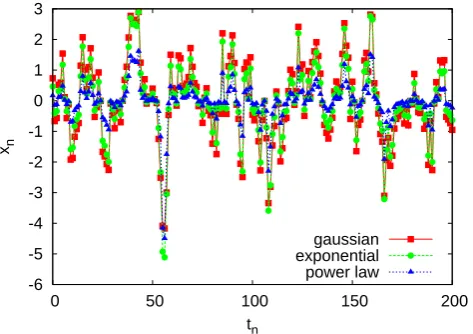
-6 -5 -4 -3 -2 -1 0 1 2 3
0 50 100 150 200
xn
tn
gaussian exponential power law
Fig. 1. Samples from the AR(1) processes with Gaussian,
exponen-tial and power-law distributions.
2.4 Constraint for increasing quality of predictions with in-creasing event magnitude
In order to study the dependence of the likelihood ratio on the event magnitude we are going to introduce a constraint which the likelihood and the total probability to find events have to fulfil in order to find a better predictability of larger (smaller) events.
In order to improve the readability of the paper, we will first introduce the following notations for the aposterior PDFs, the likelihood and the total probability to find events
ρc(η,x(n−k+1,n))=ρ(x(n−k+1,n)|Yn+1(η)=1), (10) ρf(η,x(n−k+1,n))=ρ(x(n−k+1,n)|Yn+1(η)=0), (11) L(η,x(n−k+1,n))=L(Yn+1(η)=1|x(n−k+1,n)), (12)
P (η)=P (Yn+1(η)=1). (13)
We can then ask for the change of the likelihood ratio with changing event magnitudeη.
∂
∂ηm(Yn+1(η),x(n−k+1,n))T0. (14)
The derivative of the likelihood ratio is positive (negative, zero), if the following sufficient conditionc(η)is fulfilled.
c(η,x(n−k+1,n))= ∂
∂ηlnL(η,x(n−k+1,n))− − 1
−L(η,x(n−k+1,n)))
1−P (η)
∂
∂ηlnP (η)T0. (15) Hence one can tell for an arbitrary process, if extreme events are better predictable, by simply testing, if the con-dition in Eq. (15) is positive for the respective marginal PDF of the events and the likelihood of event and precursor.
-0.2 0 0.2 0.4 0.6 0.8 1
0 20 40 60 80 100
c(
τ
)
τ
gaussian exponential power law
-16 -14 -12 -10 -8 -6 -4 -2 0
0 20 40 60 80 100
log(c(
τ
))
τ
gaussian exponential power law
Fig. 2. The autocorrelation functionc(τ )=P
n(xn−µ)(xn+τ −
µ)/((n−τ )σ2), with the meanµand the standard deviationσ is
evaluated on the AR(1) correlated data.
3 Predictions of Threshold Crossing in short range cor-related stochastic processes
In this section we test the conditionc(η,x(n−k+1,n))as given
in Eq. (15) for threshold crossing in AR(1) processes, which have a Gaussian, power-law and exponential distribution.
The most popular example for an extreme event, which consist in a threshold crossing is probably the level of water in a river, which can exceed the height of a levee and then flood an area inhabited by humans. However one can easily find other examples, in which it would be desirable to predict the exceeding of a threshold. Inspired by this motivation, we study the prediction of threshold exceedances in simple short range correlated processes. We define our extreme event by a valuexn+1of the time series exceeding a given thresholdη
Yn+1=
1, xn+1≥η,
0, xn+1< η. (16)
where the event magnitudeηis again measured in units of the standard deviation.
Due to the correlation of the AR(1) process we use the present valuexnof a time series as a precursory variable for
the event happening at timen+1.
The short range correlated processes in focus are gener-ated by an autoregressive model of order 1 [AR(1)] (see, e.g., (Box, Jenkins and Reinsel, 1994))
xn+1=axn+ξn, (17)
whereξnare uncorrelated random numbers with mean zero.
The value and the sign of the coupling strengthadetermines whether successive values of xn are clustered or spread.
considerations. Fora 6=0 the process is exponentially cor-related,hxnxn+ki=ak.
Typically the random numbersξnare chosen to be
Gaus-sian distributed. In this case the data generated by the AR(1) model is as well Gaussian distributed. However, due to the summation of random numbers in Eq. (17) also non-Gaussian random numbers might lead to a process with an approximately Gaussian distribution. That is why one has to apply other methods in order to obtain an AR(1) correlated process with a Gaussian distribution. We create the non-Gaussian distributed AR(1) processes by replacing the data of the Gaussian AR(1) process by random numbers, which follow the desired distribution function. This is done by or-dering the data of the Gaussian AR(1) process and the ran-dom numbers according to their magnitude and then replac-ing then-th largest value of the data set by then-th largest random number. This procedure lead of course to local fluc-tuations in the value of the correlations strengtha. However, the characteristic behaviour of the process is still preserved, as one can see in Figs. 1 and 2.
For the Gaussian AR(1) process all quantities which en-ter into the prediction can be evaluated analytically. Since in most cases the structure of the PDF is not know analyt-ically, we evaluatec(η, xn)also numerically. In this case
the approximations of the total probability and the likelihood are obtained by ”binning and counting” and their numeri-cal derivatives are evaluated via a Savitzky-Golay-filter (Sav-itzky and Golay, 1964; Press, 1992). The numerical eval-uation is done within 107 data points. In order to check the stability of this procedure, we evaluatec(η, xn)also on
20 bootstrap samples, which are generated from the original data set such that choosing with repetition is allowed. These bootstrap samples consist of 107 pairs of event and precur-sor, which were drawn randomly from the original data set. Thus their PDFs are slightly different in their first and second moment and they contain different numbers of events. Evalu-atingc(η, xn)on the bootstrap samples thus shows, how
sen-sitive our numerical evaluation procedure is towards changes in the numbers of events. This is especially important for large and therefore rare events.
In order to check the results obtained by the evaluation ofc(η, xn), we compute also the corresponding ROC curves
analytically and numerically.
Note that for both, the numerical evaluation of the condi-tion and the ROC-plots, we used only event magnitudesη, for which we found at least 100 events, so that the observed effects are not due to a lack of statistics of the large events. 3.1 AR(1) process with a Gaussian distribution
As it is well known, the marginal PDF of the time stepxnin
an AR(1) process is a Gaussian,
ρ(xn, a)=
s 1−a2
2π exp − 1−a2
2 xn 2
!
. (18)
Since the magnitude of the events is naturally measured in units of the standard deviation σ (a) we introduce a new scaled variableη= d
σ (a)=d
√ 1−a2.
For a 6= 0 the process is exponentially correlated hxnxn+ki=ak and the joint PDF of two successive values ρ(xn, xn+1)is a bivariate Gaussian.
From this we derive the joint PDF j (xn, Yn+1=1) by a simple integration using the Heaviside function2as a filter (see e.g. (Hallerberg et al., 2007) for details),
j (xn, Yn=1)=
Z
dxn2(xn−ησ )ρ(xn, xn+1)
The a posteriori PDFs to find or not to find events are then given by
ρc(η, xn, a)=
√
1−a2exp−1−a2
2 x 2
n
2 √
2π ρ2(a, η)
erfc
η
√ 2
√
1−a2− axn
√ 2
, (19)
ρf(η, xn, a)=
√
1−a2exp−1−a2
2 x 2
n
2 √
2π (1−ρ2(a, η))
1+erf
η
√ 2
√
1−a2 − axn
√ 2
.
(20) The corresponding likelihood reads
L(η, xn, a)=
1 2erfc
η √
2 √
1−a2 − axn
√ 2
. (21)
We recall that the optimal precursor is given byxprewhich maximises the likelihood and hencexpre=∞. In this case the alarm volume is the interval[δ,∞]. From the mean value of the aposterior PDFhxniwe can obtain the analytic structure
of the total PDF to find events
P (η, a)= a
p
2(1−a2) 1 hxni
exp −η 2
2 !
. (22)
Using
erfc(z)∼ exp(−z 2) √
π z 1+
∞
X
m=1
(−1)m1·3...(2m−1) (2z2)m
! ,
z→ ∞,|argz|<3π 4
(23)
-4 -2 0 2 4
0 5 10 15 20
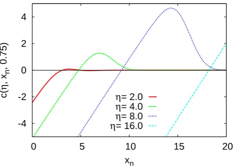
c( η , x n , 0.75) xn η= 2.0 η= 4.0 η= 8.0 η= 16.0
Fig. 3. The conditionc(η, xn,0.75)for the Gaussian distributed
AR(1) process as given by Eq. (26).
-1 -0.5 0
0 1 2 3 4 5 6 7 8 xn c( η ,xn ,0.75) η=1.96 -1 -0.5 0 η=2.32 -4 -2 0 η=2.93 -4 -2 0 2 η=3.18
Fig. 4. The analytical results (dashed light blue line) for the
Gaus-sian distributed AR(1) process are given by Eq. (26). The analyt-ical and the numeranalyt-ical results for the evaluation of the condition
c(η, xn,0.75)are compared. The results for the numerical
evalua-tion ofc(η, xn,0.75)are indicated by the symbols connected with
lines. The results for the bootstrap samples are plotted in dashed lines.
the aposterior PDF
xn∗= r
2 π
a 1−a2
exp − η √ 2 √
1−a2 − ax∗ n √ 2 2! erfc η √ 2 √
1−a2 − ax∗
n
√
2
∝ √ aη
1−a21+O1
η2
, η→ ∞, (24)
we obtain the following approximation of the total proba-bility to find events
P (η, a)∝
exp−η2 2
√ 2η
1+O
1 η2
, η→ ∞ (25)
Note that this expression is only valid in the limit of large η. In particular it does not hold forη=0. Using Eq. (21) and Eq. (25) the constraintc(xn, a, η)reads
c(η, xn, a)∝ −
s 2 π(1−a2)
exp −21
η
√
1−a2 −axn 2! erfc η √ 2 √
1−a2 − ax√n
2
+
η+1 η
1−1 2erfc η √ 2 √
1−a2 − axn
√
2
1−exp(−η√ 2/2)
2η
1+O1 η2
(26) Using again Eq. 23 we obtain the following asymptotic behaviour for large values ofη
c(η, xn, a)→η
1−O exp(−η2)/η 1−O exp(−η2)/η !
−√ 1 1−a2
!
+√axn 1−a2
1 1+O(1/η2) +1
η
1−O exp(−η2)/η 1−O exp(−η2)/η !
, η→ ∞. (27)
This expression is larger than zero, if terms of the order O exp(−η2)/η
are negligible. Hence we can conclude, that c(η, xn, a)is positive for large values ofηand arbitrary
val-ues ofxn.
However for finite values ofηwe observe a dependence on the precursory variable. Figures 3 and 4 display that c(η, xn, a)is positive for larger values, i.e., values, which are
closer to the ideal precursorxpre=∞. Hence we should ex-pect larger events to be better predictable, if our alarm inter-val is situated in this region, i.e., if the alarm interinter-val[δ,∞] is small.
The ROC curves in Fig. 5 support this result. In the region of low rates of false alarms which corresponds to a small alarm interval we find a strong dependence on the event mag-nitude in the sense, that larger events are better predictable.
Finally one can discuss the case of the ideal precursor xpre=∞. Inserting this value of the precursory variable into Eq. 26 one obtainsc(η, xn, a)=0. This ideal precursor
0 0.2 0.4 0.6 0.8 1
0 0.1 0.2 0.3 0.4 0.5 0.6 0.7 0.8 0.9 1
rate of correct predictions
rate of false alarms η = 0.00 η = 0.94 η = 1.88 η = 2.81
η = 3.75
Fig. 5. ROC curves for the Gaussian distributed AR(1) process with correlation coefficienta=0.75. The ROC curves where made via predicting threshold crossings of magnitudeηwithin 107data points. The predictions were made according to the prediction strat-egy described in Sect. 2.1. Note that the quality of the prediction increases with increasing event magnitude.
3.2 AR(1) Process with Symmetrised Exponential Distri-bution
The AR(1) data with exponential distribution were created via replacing the values of the Gaussian distributed AR(1) data with exponentially distributed i.i.d. random variables, as explained in Sect. 3. The exponential distributed AR(1) process has the following PDF
ρ(x)= λ
2exp(−λ|xn|)
withλ=1 and was generated by transformation from uni-formly distributed random numbers. (The uniuni-formly dis-tributed random numbers were generated by using the Mersenne twister algorithm (Matsumoto and Nishimura, 1998).) Numerically we find the maximum of the likelihood also in the region of large values ofxn, similar to the
Gaus-sian case with an alarm interval[δ,−∞]. We compute the condition according to Eq. (15) and the ROC curves numer-ically by using 107exponential distributed AR(1) correlated data.
Figure 6 compares the results of the numerical evaluation of the conditionc(η, xn, λ). In the vicinity of the larger
val-ues of the data set, the conditionc(η, xn, λ)is positive as in
the Gaussian case.
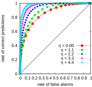
The ROC curves in Fig. 7 support the qualitative results from Fig. 6, that larger events are better predictable. The numerical ROC curves were made via predicting threshold crossings in 107AR(1) correlated exponentially distributed data points according to the prediction strategy described in Sect. 2.1.
-2 -1 0
0 2 4 6 8 10 12 14 xn
c(
η
,xn
)
η=3.0 -2
-1 0
η=3.57 -4
-2 0 η=4.51 -4
-2 0 2
η=4.89
Fig. 6. The condition according to Eq. (15) evaluated on 107 expo-nentially distributed AR(1) correlated data .
0 0.2 0.4 0.6 0.8 1
0 0.1 0.2 0.3 0.4 0.5 0.6 0.7 0.8 0.9 1
rate of correct predictions
rate of false alarms
η = 0.00
η = 1.1
η = 2.2
η = 3.3
η = 4.4
Fig. 7. The ROC curves where made via predicting threshold
cross-ings in 107 exponentially distributed AR(1) correlated data and the predictions were made according to the prediction strategy de-scribed in Sect. 2.1.
This result is qualitatively different from the results of prediction of increments in sequences of exponentially dis-tributed i.i.d. random numbers in (Hallerberg et al., 2007). In this previous work we found that the event magnitude has no influence on the prediction of large increments in sequences of exponentially distributed i.i.d. random numbers. This dif-ference can probably be understood by the fact that the con-ditionc(η, xn)is not only a function of the event magnitude η, but also a function of the event class and of the precursor valuesxn.
3.3 Power-law distributed random variables
-1 -0.5 0 0.5
0 10 20 30 40 50 60 70 80 xn
c(x
n
,
η
, 0.75)
η=1.55 -0.5
0
η=2.24 -0.2 0
0.2
η=3.45 -0.3
0 0.3 0.6
η=4.48
Fig. 8. The conditionc(η, xn, α, σ )evaluated on 107power-law
distributed AR(1) correlated data with varianceσ=1, mean zero and power-law coefficientα=3.xn.
with symmetrised power-law distributed i.i.d. random vari-ables, as explained in Sect. 3.
The symmetrised power-law distributed i.i.d. random vari-ables follow the following distribution
ρ(x)=αxminα x−(α+1), x > xmin>0
ρ(x)=α|xmax|α|x|−(α+1), x < xmax<0, (28)
with xmin=|xmax|=0.01 and power-law coefficient α=3 were generated by transformation from uniformly dis-tributed random numbers. Since the distributions with xmin = |xmax|=0.01 would allow no values in the interval ]xmin, xmax[, the resulting random numbers were shifted to the left (right) by subtracting (adding) xmin. The result is a symmetrised power law distribution with mean zero and varianceσ=0.01, see Figs. 1 and 2. Finally, the values of the AR(1) process were amplified by multiplication with a con-stantca=100, so that the data set of the power law distributed
AR(1) process has a variance ofσ=1, as the Gaussion and the exponential AR(1) process.
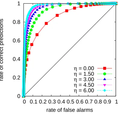
Figures 8 and 9 show the numerical results for c(η, xn, α, σ )and the ROC curves.
Althoughc(η, xn, α, σ )is less regular than in the
Gaus-sian or the exponential case, its values are mainly above zero which corresponds to the ROC curves in Fig. 9.
Hence large threshold crossings are also within the Pareto distributed AR(1) process better predictable than smaller. As in the exponential case, this result for threshold crossings in AR(1) correlated data is qualitatively different from the re-sults for the prediction of increments in sequences of Pareto distributed random numbers.
0 0.2 0.4 0.6 0.8 1
0 0.1 0.2 0.3 0.4 0.5 0.6 0.7 0.8 0.9 1
rate of correct predictions
rate of false alarms
η = 0.00
η = 1.50
η = 3.00
η = 4.50
η = 6.00
Fig. 9. ROC-plot for the power-law distribution. The ROC curves
where made via predicting increments in 107 data points of the AR(1) process with power-law distribution.
4 Predicting Threshold Crossings in Free Jet Data
In this section, we apply the method of statistical inference to predict threshold crossings of the acceleration in a free jet flow. Therefore we use a data set of 1.25×10⁷samples of the local velocity measured in the turbulent region of a round free jet (Renner, Peinke and Friedrich, 2001). The data were sampled by a hot-wire measurement in the central region of an air into air free jet. One can then calculate the PDF of ve-locity differencesan,k=vn+k−vn, wherevnandvn+kare the
velocities measured at time stepnandn+k. The Taylor hy-pothesis allows to relate the time-resolution to a spatial res-olution (Renner, Peinke and Friedrich, 2001). One observes that for large values ofkthe PDF of the velocity differences is essentially indistinguishable from a Gaussian, whereas for smallk, the PDF develops approximately exponential wings (Van Atta and Park, 1972; Gagne et al., 1990; Frisch, 1995). Figure 10 illustrates this effect using the data set under study. Thus the incremental data setsan,k provides us with the
opportunity to test the results for statistical predictions within Gaussian and exponential distributed AR(1) correlated pro-cesses on a data set, which exhibits correlated structures.
We are now interested in predicting larger values of the acceleration an+j,k≥η in the incremental data sets an,k=vn+k−vn. In the following we concentrate on the data
-15 -10 -5 0 5
-2 -1.5 -1 -0.5 0 0.5 1 1.5 2 2.5
log
ρ
(vn+k
- v
n
)
vn+k - vn
k=1 k=3 k=10 k=35 k=144 k=285
Fig. 10. PDF of the accelerationsan,k=vn+k−vnwith k=1, 3, 10,
35, 144, 285.
-0.05 0
0.5 0.6 0.7 0.8 0.9 1
xn
c(
η
,xn
)
k=10 j=2
η=3.07
-0.05 0
η=3.65
-0.2 0
η=4.42
-0.5 -0.25 0
η=5.0
(a)
-0.2
-0.1 0
0.1
0.9 1.2 1.5 1.8
xn
c(
η
, x
n
)
k=144
j=7
η=2.3
-0.4
-0.2 0 η=2.73
-0.5 0
η=3.01
-0.5 0
η=3.88
(b)
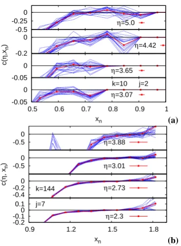
Fig. 11. The condition c(η, an,k) evaluated in the exponential
regime (k=10) (a) and in the Gaussian regine (k=144) (b).
and the precurser, but also the predition horizon influences the resulting ROC curves.
As in the previous sections we are hence exploiting the conditional probabilities of the time series to make predic-tions. We can now use the algorithm which was tested on the previous examples to evaluate the condition for these data sets. The results are shown in Fig. 11. In both examples the evaluation of the conditionc(η, an,k)reflects the behaviour
of the ROC curves. This example of the free jet data-set shows, that the specific dependence of the ROC curve on the
0 0.2 0.4 0.6 0.8 1
0 0.2 0.4 0.6 0.8 1
rate of correct predictions
rate of false alarms k=10
j=2
η = 0.00
η = 1.44
η = 2.89
η = 4.32
η = 5.76
(a)
0 0.2 0.4 0.6 0.8 1
0 0.2 0.4 0.6 0.8 1
rate of correct predictions
rate of false alarms k=144
j=7
η = 0.0 η = 1.1 η = 2.2 η = 3.3 η = 4.4
(b)
Fig. 12. ROC curves in the exponential (k=10) (a) and in the
Gaus-sian regime (k=144) (b).
event magnitude can also in the case of long-range correlated data sets be characterised by the PDF of the underlying pro-cess.
5 A more realistic prediction procedure
Predicting an above-threshold event when the current obser-vation itself is already above the threshold might not be really relevant in most applications.
We therefore modify here the sample on which predictions are to be made: We define as events the subset of previous events, where not only the future value is above threshold, but simultaneously the current value is below threshold. Yn+1=
1 :xn+1≥η, xn< η
0 :xn+1< η, xn< η
(29) The events Yn=1 according to this definition are a subset
0 0.2 0.4 0.6 0.8 1
0 0.1 0.2 0.3 0.4 0.5 0.6 0.7 0.8 0.9 1
rate of correct predictions
rate of false alarms η = 0.00 η = 0.94 η = 1.88 η = 2.81 η = 3.75
Fig. 13. ROC curves for the Gaussian AR(1) process made
accord-ing to the more realistic prediction procedure described in Sect. 5.
0 0.2 0.4 0.6 0.8 1
0 0.1 0.2 0.3 0.4 0.5 0.6 0.7 0.8 0.9 1
rate of correct predictions
rate of false alarms η = 0.00 η = 1.41 η = 2.82 η = 4.23 η = 5.64
Fig. 14. ROC curves for the exponential distributed AR(1) process
made according to the more realistic prediction procedure described in Sect. 5
curves obtained in the previous section: Threshold crossings in Gaussian, approximately exponential distributed, and ap-proximately power-law distributed AR(1) processes are bet-ter predictable, the larger they are.
6 Conclusions
We study the magnitude dependence of the quality of pre-dictions for threshold crossings in autocorrelated processes of order one and in measured accelerations in a free jet flow. Using the present valuexnas a precursory variable we
pre-dict threshold crossings at a future time stepxn+j via
statis-tical considerations. In order to measure the quality of the
0 0.2 0.4 0.6 0.8 1
0 0.1 0.2 0.3 0.4 0.5 0.6 0.7 0.8 0.9 1
rate of correct predictions
rate of false alarms
η = 0.00
η = 1.50
η = 3.00
η = 4.50
η = 6.00
Fig. 15. ROC curves for the power law distributed AR(1) process
made according to the more realistic prediction procedure described in Sect. 5.
predictions we use ROC curves. Furthermore, we introduce a quantitative criterion which can determine, whether larger or smaller events are better predictable.
We are especially interested in the influence of the prob-ability distribution of the underlying process on changes in the quality of the predictions, which are evoked by focus-ing on different event magnitudes. For Gaussian, exponen-tial and power law distributed AR(1) processes we find, that larger threshold crossings are better predictable, the higher the threshold. In all cases studied the behaviour of the ROC curves was reasonably well reflected by the condi-tionc(η, xn), which is an expression that depends on the
to-tal probability to find events and the likelihood to observe an event after a given value ofxn. This theoretical results
could in principle help to understand the effects reported for avalanches in systems, which display self organized critical-ity (Shapoval and Shrirman, 2006).
The velocity measurements in the free jet flow provide us with the opportunity to redo the predictions in data sets, which inhibits correlated structures, and have either asymp-totically Gaussian or asympasymp-totically exponential distribu-tions.
In both cases larger threshold crossings are also in the free jet data set better predictable, the higher the threshold.
This difference to the recent results for threshold crossings can be explained by taking into account the different regimes in which we find the optimal precursors:
When predicting increments, the optimal precursors are typically among the smallest values in the data set, while for the prediction of threshold crossings, large values are opti-mal. Furthermore threshold crossings form a different class of events. Hence both PDFs which contribute to the value ofc(η, xn), namely the likelihood and the total probability to
find events are different. Hence we should not be surprised to find different results for the predictability of larger events. In summary we find, that threshold crossings in AR(1) pro-cesses and also in the correlated free jet flow data are the better predictable, the larger they are.
Acknowledgements. We thank J. Peinke and his group for supply-ing us with their excellent free jet data.
Edited by: S. Vannitsem
Reviewed by: two anonymous referees
References
Jackson, D. J.: Hypothesis testing and earthquake prediction, Proc. Natl. Acad. Sci. USA, 93, 3772–3775, 1996.
Kantz, H., Holstein ,D., Ragwitz, M., and Vitanov, N. K.: Markov chain model for turbulent wind speed data, Physica A, 342, 315– 321, 2002.
Kantz, H., Holstein, D., Ragwitz, M., and Vitanov, N. K.: Short time prediction of wind speeds from local measurements, in: Wind Energy–Proceedings of the EUROMECH Colloquium, edited by: Peinke, J., Schaumann, P., and Barth, S., Springer, 2006.
Hallerberg, S., Altmann, E. G., Holstein, D., and Kantz, H.: Precur-sors of Extreme Increments, Phys. Rev. E, 75, 016706, 2007. Shapoval, A. B. and Shrirman M. G.: How size of target avalanches
influence prediction efficiency, Int. J. Mod. Phys. C, 17, 1777– 1790, 2006.
Hallerberg, S. and Kantz, H.: Influence of the Event Magnitude on the Predictability of Extreme Events, Phys. Rev. E, 77, 011108, 2008.
Lamper, D., Howison, S. D., and Johnson N. F.: Predictability of large future changes in a competitive evolving population, Phys. Rev. Lett., 88, 1, 2002.
Box, G. E. P., Jenkins G. M., and Reinsel G. C.: Time Series Anal-ysis, Prentice-Hall, Inc., 1994.
Brockwell, P. J. and Davis, R. A.: Time Series: Theory and Meth-ods, Springer, 1998.
Hallerberg, S., Br¨ocker, J., and Kantz, H.: Prediction of Extreme Events, accepted for publication in Nonlinear Time Series Analy-sis in the Geosciences-Applications in Climatology, Geodynam-ics, and Solar-Terrestrial PhysGeodynam-ics, edited by: Donner, R. and Bar-bosa, S.: Lecture Notes in Earth Sciences, Springer, accpeted, 2008.
Egan, J. P.: Signal detection theory and ROC analysis, Academic Press, New York, 1975.
Green, D. M. and Swets J. A.: Signal detection theory and psy-chophysics, Wiley, New York, 1966.
Pepe M. S.: The Statistical Evaluation of Medical Tests for Classi-fication and Prediction, Oxford University Press, 2003. Savitzky, A. and Golay, M. J. E.: Smoothing and Differentiation of
Data by Simplified Least Squares Procedures, Anal. Chem., 36, 1627–1639, 1964.
Press, W. H.: Numerical recipes in C, Cambridge University Press, Cambridge, 1992.
Abramowitz, M. and Stegun, I. A.: Handbook of Mathematical Functions, Dover, New York, 1972.
Matsumoto, M. and Nishimura, T.: Mersenne Twister: A 623-dimensionally equidistributed uniform pseudorandom number generator, in ACM Transactions on Modeling and Computer Simulation, 8, 1, 3–30. 1998.
Renner, C., Peinke, J. and Friedrich, R.: Experimental indications for Markov properties of small-scale turbulence, J. Fluid. Mech., 433, 383–09, 2001.
Van Atta, C. W. and Park, J.: Statistical self-similarity and intertial subrange turbulence, in Statistical Models and Turbulence, Lect. Notes in Phys., 12, 402–426, edited by: Rosenblatt, M. and Van Atta, C. W., Springer Berlin, 1972.
Gagne, Y., Hopfinger, E., and Frisch, U.: A new universal scal-ing for fully developed turbulence: the distribution of velocity increments, in New Trends in Nonlinear Dynamics and Pattern-Forming Phenomena, NATO ASI, 237, 315–319, edited by: Coullet, P. and Huerre, P., Plenum Press, New York, 1990. Frisch, U.: Turbulence, Cambridge University Press, Cambridge,