Dynamics of turbulence under the effect of stratiﬁcation and internal waves

(1)

www.nonlin-processes-geophys.net/22/337/2015/ doi:10.5194/npg-22-337-2015

Dynamics of turbulence under the effect of stratification

and internal waves

O. A. Druzhinin1and L. A. Ostrovsky2

1_{The Institute of Applied Physics, Russian Acad. Sci., Nizhny Novgorod, Russia} 2_{NOAA Environmental Science Research Lab., Boulder, CO, USA}

Correspondence to: O. A. Druzhinin ([email protected])

Received: 29 December 2014 – Published in Nonlin. Processes Geophys. Discuss.: 19 February 2015 Revised: 27 April 2015 – Accepted: 12 May 2015 – Published: 4 June 2015

Abstract. The objective of this paper is to study the dynam-ics of small-scale turbulence near a pycnocline, both in the free regime and under the action of an internal gravity wave (IW) propagating along a pycnocline, using direct numeri-cal simulation (DNS). Turbulence is initially induced in a horizontal layer at some distance above the pycnocline. The velocity and density fields of IWs propagating in the pyc-nocline are also prescribed as an initial condition. The IW wavelength is considered to be larger by the order of mag-nitude as compared to the initial turbulence integral length scale. Stratification in the pycnocline is considered to be suf-ficiently strong so that the effects of turbulent mixing remain negligible. The dynamics of turbulence is studied both with and without an initially induced IW. The DNS results show that, in the absence of an IW, turbulence decays, but its decay rate is reduced in the vicinity of the pycnocline, where strati-fication effects are significant. In this case, at sufficiently late times, most of the turbulent energy is located in a layer close to the pycnocline center. Here, turbulent eddies are collapsed in the vertical direction and acquire the “pancake” shape. IW modifies turbulence dynamics, in that the turbulence kinetic energy (TKE) is significantly enhanced as compared to the TKE in the absence of IW. As in the case without IW, most of the turbulent energy is localized in the vicinity of the py-cnocline center. Here, the TKE spectrum is considerably en-hanced in the entire wave-number range as compared to the TKE spectrum in the absence of IW.

1 Introduction

Interaction between small-scale turbulence and internal grav-ity waves (IWs) plays an important role in the processes of mixing that have a direct impact on the dynamics of the seasonal pycnocline in the ocean (Phillips, 1977; Fernando, 1991). Turbulence in the mixed region above the pycnocline can be produced by breaking surface waves driven by the wind forcing or due to shear-flow instabilities. In laboratory studies of the effect of small-scale turbulence on the pycn-ocline, in the absence of mean shear, turbulent motions are usually induced by an oscillating grid (Turner, 1973; Thorpe, 2007).

(2)

338 O. A. Druzhinin and L. A. Ostrovsky: Effect of stratification and internal waves

The effect of damping of IWs propagating through a py-cnocline by a forced turbulent layer above the pypy-cnocline was recently studied with the use of direct numerical sim-ulation (DNS) by Druzhinin et al. (2013). The results show that if the ratio of IW amplitude to turbulent pulsations amplitude is sufficiently small (less than 0.5), turbulence strongly enhances IW damping. In this case, the damping rate obtained in DNS agrees well with the prediction of a semi-empirical closure approach developed by Ostrovsky and Zaborskikh (1996). However, for larger IW amplitudes, the effect of damping of IWs by turbulence is much weaker, and, in this case, the semi-empirical theory overestimates the IW damping rate by the order of magnitude.

The effect of enhancement of small-scale turbulence by mechanically generated, non-breaking internal waves was experimentally observed by Matusov et al. (1989). In that experiment, an oscillating grid was used to induce turbulence above a pycnocline. An internal gravity wave propagating in the pycnocline was generated by a wave maker. The results of this experiment show that a sufficiently strong (as com-pared to turbulent grid-induced velocity fluctuations), non-breaking internal wave can significantly increase the kinetic energy of turbulence in the well-mixed layer above the py-cnocline. However, the obtained experimental data did not provide enough detail to study the modification of turbulence kinetic energy spectra under the influence of IWs.

A somewhat similar phenomenon has been experimentally observed in the ocean boundary layer where the kinetic en-ergy of turbulence and its dissipation rate can be signifi-cantly enhanced in the presence of surface gravity waves rel-ative to the wind-stress production (cf., e.g., Anis and Moum, 1995). The results of recent numerical simulations by Tsai et al. (2015) also show that non-breaking surface waves can ef-fectively increase turbulence kinetic energy in the vicinity of the water surface.

The objective of the present paper is to study the possibil-ity of the enhancement of small-scale turbulence by an in-ternal gravity wave (IW) propagating in a pycnocline, and to consider the case where the initial IW amplitude is on the order of, or larger than, the turbulent pulsation amplitude. The results of DNS by Druzhinin et al. (2013) show that, un-der this condition, the damping of IW by turbulence remains negligible. As in the latter study, the buoyancy jump across the pycnocline is considered to be large enough, such that the effects related to turbulent mixing remain insignificant. The main focus here is to investigate in more detail the ef-fect of the enhancement of small-scale turbulence by an IW propagating in the pycnocline, and, in particular, to separate the contributions of the IW velocity field and the turbulent velocity field produced by the IW in the fluid kinetic energy spectrum.

The setup and parameters of the numerical experiment are discussed in Sect. 2. Initialization of internal waves and their properties are discussed in Sect. 3. The dynamics of turbu-lence in the absence of the initially excited IW is discussed

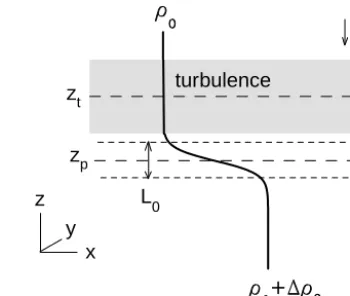
N₀ z turbulence L 0 g x y z_p z_t

Figure 1. Schematic of the numerical experiment:x,yandzare the Cartesian coordinates;ρ0is the density above the pycnocline;1ρ0

the density jump across the pycnocline;gthe gravity acceleration,

N0the buoyancy frequency in the pycnocline center;L0the

pycn-ocline thickness;zpandztthe locations of the pycnocline and the

turbulent layer centers.

in Sect. 4. The effect of an IW propagating in the pycnocline on turbulence dynamics is discussed in Sect. 5. Conclusions and discussion of numerical results and estimates of the en-hancement of small-scale turbulence by IWs in laboratory and natural conditions are presented in Sect. 6.

2 Numerical method and initial conditions

We consider a stably stratified fluid with a pycnocline (Fig. 1). The initial turbulence field is localized in a layer at some distance above the pycnocline. The first mode of the internal wave propagating along the pycnocline from left to right is also prescribed as an initial condition. Periodic boundary conditions in the horizontal,xandy, directions and a Neumann (zero normal gradient) boundary condition in the verticalzdirection are considered. The thickness of the py-cnocline,L0, and the buoyancy frequency in the middle of the pycnocline,N0=

−g

ρ0 dρ0

dz 1/2

(where gis the gravity acceleration andρ0(z)the fluid density), are chosen to define the characteristic length and timescales,L0andT0=1/N0, which are used further to write the governing equations in the dimensionless form.

The Navier–Stokes equations for the fluid velocity are written under the Boussinesq approximation as (Phillips, 1977)

∂Ui ∂t +Uj

∂Ui ∂xj

= −∂P

∂xi

+ 1

Re ∂2Ui

∂x_j2

−Riδizρ, (1)

∂Uj ∂xj

=0. (2)

(3)

∂ρ ∂t +Uj

∂ρ ∂xj

−UzNref2 (z)= 1 ReP r

∂2ρ

∂x_j2. (3)

In Eqs. (1)–(3),Ui (i=x, y, z)is the instantaneous fluid ve-locity, and ρ andP are the instantaneous deviations of the fluid density and pressure from the respective hydrostatic profiles;xi=x, y, zare the Cartesian coordinates.

Reynolds and Richardson numbers are defined as

Re=U0L0

ν , Ri=

_L

0N0 U0

2

. (4)

The Prandtl number isP r=ν/κ, whereνis the fluid kine-matic viscosity andκ the molecular diffusivity. The coordi-nates, time and velocity are normalized by the length scales, timescales and velocity scales,L0,T0andU0=L0/T0. Note that, since the timescale is defined asT0=1/N0and the ve-locity scale asU0=L0/T0=L0N0, the Richardson number in DNS identically equals unity,Ri=1. The density devia-tion ρis normalized by the density jump across the pycno-cline,1ρ0(Fig. 1).

The dimensionless reference profile of the buoyancy fre-quency,Nref(z), is prescribed in the form

Nref(z)= 1

cosh 2(z−zp), (5)

wherezpdefines the pycnocline location, and the dimension-less reference density profile,ρref(z), is

ρref(z)=ρref(−∞)−

z Z

−∞

N_ref2 (z)dz=ρref(−∞)

−0.5 tanh 2(z−zp), (6)

whereρref(−∞)can be an arbitrary constant since its value does not influence the integration of Eqs. (1)–(3). Thus, for convenience,ρref(−∞), is set equal to 1.5, and the reference density profile is rewritten in the form

ρref(z)=1+0.5

1−tanh 2(z−zp). (7)

The dimensionless instantaneous density is obtained as a sum of ρref(z) and the instantaneous density deviation, ρ. Note that the dimensional density can be obtained as a sum

ρ0+1ρ0 0.5[1−tanh 2(z−zp)] +ρwhereρ0is the di-mensional reference (undisturbed) density above the pycno-cline.

The Navier–Stokes equations for the fluid velocity and density Eqs. (1)–(3) are integrated into a cubic domain with sizes 0≤x≤40,−10≤y≤10 and 0≤z≤20 by employ-ing a finite difference method of second-order accuracy on a uniform rectangular staggered grid consisting of 400×200×

200 nodes in thex,y andzdirections, respectively. The in-tegration is advanced in time using the Adams–Bashforth

method with time step1t=0.01. The Poisson equation for the pressure is solved by FFT transform over thexandy co-ordinates, and the Gaussian elimination method over thez coordinate (Druzhinin et al., 2013). The Neumann (zero nor-mal gradient) boundary condition is prescribed for all fields in the horizontal (x, y)planes atz=0 andz=20, and peri-odic boundary conditions are prescribed in the longitudinal (x)and transverse (y)directions.

In DNS, we prescribe the Reynolds number to be Re=20 000. This number is sufficiently large to render the viscous damping of IWs negligible. The Prandtl numberP r is set equal to unity.

3 Internal waves

The initial condition for the velocity and density fields is pre-scribed as a first mode of internal wave field with wavelength λ(and wave numberk=2π/λ)and frequencyω. The solu-tion of the linearized Eqs. (1)–(3) for the progressive internal wave propagating from left to right in thexdirection can be defined as (Phillips, 1977)

U_xI W(x, z, t )= −1

k dW (z)

dz sin(kx−ωt ), (8)

U_zI W(x, z, t )=W (z)cos(kx−ωt ), (9) ρ_zI W(x, z, t )=W (z)

ω dρref

dz sin(kx−ωt ). (10)

The initial conditions for the IW field are taken from Eqs. (8)–(10) att=0. FunctionW (z)is obtained as an eigen-function of the well-known Taylor–Goldstein boundary prob-lem (Phillips, 1977):

d2W dz2 +

N2 ω2 −1

k2W=0, (11)

with conditionsW (z)→W0expk(z−zp)forzzp, and W (z)→W0exp

−k(z−zp)

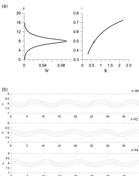
for zzp, where W0 is the IW velocity amplitude atz=zp. The problem Eq. (11) was solved by the shooting method with matching at the pycn-ocline center,z=zp (Hazel, 1972). The distribution of the first-mode vertical velocity in the IW and the dispersion re-lationω(k)for wave numbers in the range 0.3< k <6 ob-tained numerically for wavelength λ=10 are presented in Fig. 2a. The figure shows that, as expected, the energy of the first mode is concentrated around the pycnocline.

DNS was performed with initial conditions Eqs. (8)–(10) att=0 corresponding to the IW fields with wavelengthλ=

(4)

Figure 2. (a) Distribution of the vertical velocityW (z)for wave-lengthλ=10 (left) and the dispersion relationω(k)(right) for the first IW mode. The wave number of the selected wavelength is shown by a symbol. (b) The instantaneous contours of the den-sity deviation obtained in the central (x, z)plane at different time moments in DNS with initial condition (Eqs. 5–7) prescribed for IW, propagating from left to right with wavelength λ=10 (fre-quencyω=0.489, phase velocityc≈0.78) and amplitudeW0=

0.1. There is no initially induced turbulence. Density contours are 1.3, 1.5 and 1.7. Contour 1.5 marks the location of the pycnocline center.

IW amplitudes and reduce the IW length, the wave slope increases so that strong, short-length IWs become strongly nonlinear and are prone to breaking and viscous dissipa-tion. In the present study, the IW amplitude was prescribed as W0=0.1. Figure 2b shows isopycnal displacements ob-tained in DNS at different times with initial conditions pre-scribed for an IW with selected wavelength. In this case, the amplitude of the isopycnal displacement is about a≈0.2, and the wave slope is aboutka=2π a/λ≈0.12, which may be regarded as small enough to ensure that nonlinear effects during the IW propagation in the pycnocline remain negligi-ble. Below (in Fig. 7), spatial IW spectra also show that am-plitudes of higher harmonics remain negligible as compared to the first-harmonics amplitude.

4 Dynamics of turbulence in the absence of IW

In order to investigate how turbulence evolves in the absence of internal waves, DNS was performed with the initially in-duced turbulence field and no imposed IW field. The mid-pycnocline level was prescribed atzp=8 and the turbulence layer center was set atzt=10. The values ofzpandztwere chosen to ensure that the effects of turbulent mixing and in-ternal wave generation by turbulence in the pycnocline re-mained sufficiently small for the considered initial amplitude of turbulent velocity (defined below).

The turbulent velocity field is initialized in DNS as a ran-dom, divergence-free field in the form

Ui(x, y, z)=Ut0U_if(x, y, z)exp h

−0.5(z−zt)2)i, (12) wherei=x,y,z.U_if(x, y, z)is a homogeneous isotropic field with a given power spectrum in the form

E(k)=E0kexp

−k

kf

, (13)

where wave numberkf defines the spectral location of the energy peak. FactorE0is chosen so that the amplitude (i.e., an absolute maximum value of the modulus ofU_if(x, y, z)) equals unity. Thus, parameter Ut0 in Eq. (12) defines the turbulence velocity amplitude; Ut0 andkf were prescribed in DNS as Ut0=0.1 and kf =1. Numerical results show that, in this case, the effects of turbulent mixing on the py-cnocline structure and generation of internal waves by tur-bulence remain negligible during the considered time inter-val (0< t <400 in dimensionless units). For the considered choice of the spectrum given by Eq. (13) withkf=1 the tur-bulence dimensionless integral length scale,Lt, at initializa-tion is on order unity. Thus, the turbulent Reynolds number, Ret, based onLtandUt0, is evaluated asRet=LtUt0Re≈

2000.

The mean vertical profiles of the velocity and density fields,< Ui> (z)and< ρ > (z), were obtained by averag-ing over the horizontal (x, y) plane performed for each z. Root mean square (rms) deviations of the velocity and den-sity were then obtained as

U_i0=< U_i2−< Ui>2> 1/2

, ρ0

=< ρ2−< ρ>2> 1/2

. (14)

The vertical mean profile of the mean kinetic energy,E(z), was evaluated as

E=1

2

X

i=x,y,z

U_i02. (15)

(5)

number,Rig(Phillips, 1977). In the considered case, there is no mean shear. Thus, the gradient Richardson number param-eter can be evaluated via the mean buoyancy frequency,N, and the mean turbulent shear stress defined by the TKE dis-sipation rate and kinematic viscosity,(ε/ν≡εRe)(Thorpe, 2007), as

Rig= − Ri εRe

d < ρ >

dz =

N2

εRe, (16)

where the dissipation rate,ε, can be obtained from DNS data by averaging over the (x, y) plane for each z in the form (Phillips, 1977)

ε= 1

Re

X

i

< ∂Uei ∂x

!2

+ ∂Uei

∂y

!2

+ ∂Uei

∂z

!2

> (17)

In Eq. (17), Uei =Ui−< Ui>, i=x,y,zis the instanta-neous deviation of the velocity from the mean value.

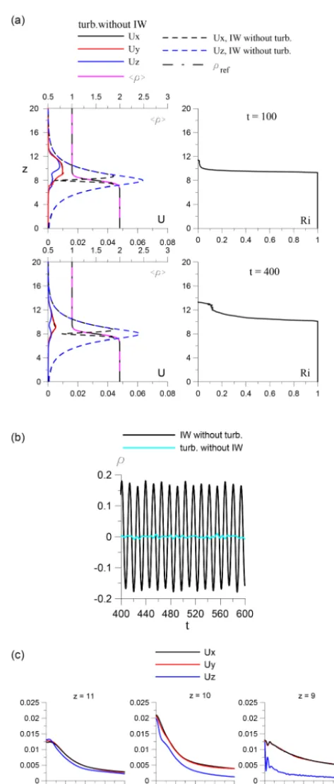
Figure 3a shows vertical profiles of different rms velocity components,U_x0,U_y0 andU_z0, and mean density,< ρ >(left panel), and the Richardson number, Rig (right panel), ob-tained in DNS at time momentst=100 andt=400 with no initially induced IW. (Here and below in Fig. 4a, theRig(z) profile is cut off at the level of unity forRig(z) >1.) The fig-ure also shows the density reference (initial) profile,ρref(z), and the profiles of the rms velocity components U_x0 andU_z0 of the internal wave without an initially induced turbulence layer. The figure shows thatx andyrms velocities coincide in the region sufficiently far from the pycnocline (forz >11). In this region, the gradient Richardson number remains suf-ficiently small (Rig<0.2 att=400), so that it can be re-garded as weakly stratified. On the other hand, in the region z <10, sufficiently close to the pycnocline,Rig>1 and ver-tical rms velocity,U_z0, are much smaller as compared to the horizontal rms velocities,U_x0 andU_z0, whose amplitudes peak at levelz=9 att=400. Thus, in this strongly stratified re-gion, turbulent motion becomes quasi-two-dimensional and there is a collapse of three-dimensional vortices and the for-mation of pancake eddies (cf. Fig. 3e below). Figure 3a also shows that the mean density profile, < ρ > (z), practically coincides with the reference profile,ρref(z), during the con-sidered time interval. That means that the effect of turbulent mixing on the pycnocline structure remains negligible.

Figure 3a also shows that vertical rms velocity increases in the vicinity of the pycnocline center (at z=8) where U_x0, U_y0, U_z0 are on the same order. This increase can be at-tributed to the presence of internal waves excited by de-caying turbulence in the pycnocline. The presence of these turbulence-generated IWs is confirmed by numerical results in Fig. 3b. The figure shows temporal development of the density at the point with coordinatesx=20,y=10 andz=8 (i.e., at the pycnocline center in the middle of the computa-tional domain). The figure also shows the temporal devel-opment of the density in an initially induced internal wave

without initially excited turbulence for comparison. The fig-ure shows that small, finite density variations are present in the pycnocline, which can be attributed to weak internal waves excited by turbulence. The analysis of the frequency spectrum of the density oscillations in the pycnocline and the structure of isopycnals (not presented here) shows that mostly first- and second-mode IWs are generated by turbu-lence with corresponding frequenciesω1≈0.8 andω2≈0.2 and wavelength λt≈4. (More details about the physical mechanism responsible for the IW generation by turbulence in a pycnocline are provided, e.g., by Kantha, 1979, and Car-ruthers and Hunt, 1986). The amplitude of these turbulence-generated IWs remains smaller by the order of magnitude as compared to the amplitude of the IW induced in the pycno-cline due to the initial condition (Eqs. 8–10).

Figure 3c shows the temporal development ofx,y andz rms velocity components, U_x0, U_y0, U_z0, obtained in DNS at differentzlevels (z=9, 10 and 11). The figure shows that turbulence decays, and the decay rate is different at different zlevels. At z=11, the rms velocities remain on the same order at all times. At levelsz=10 andz=9, componentU_z0 diminishes at a greater rate as compared to thexandy com-ponents,U_x0andU_y0, so that at sufficiently late times (t >200 for z=10 and t >50 atz=9), vertical velocity becomes smaller almost by the order of magnitude as compared to thexandy-velocity components. That means that in the re-gion sufficiently close to the pycnocline, there is a collapse of three-dimensional turbulence under the effect of stable strat-ification and fluid motion becomes quasi-two-dimensional.

Temporal development of the mean kinetic energy,E, at differentzlevels (z=9, 10 and 11), is presented in Fig. 3d. The figure shows thatEdecays at a lower rate in the region in the vicinity of the pycnocline (atz=9) as compared to levels z=10 and z=11 where stratification is weak. The figure shows that E(z=11)∼t−1.6, whereas E(z=9)∼t−0.9 at timest >50.

(6)

Figure 3. (a) Vertical profiles of the rms velocity components,U_x0,U_y0 andU_z0, mean density< ρ >(left) and the gradient Richardson number,Rig (right), obtained at time momentst=100 andt=100 in DNS with no initially induced IW. The reference (initial) density

profile,ρref(z), is shown in dash-dotted (black) line for comparison. Profiles of the rms velocityxandzcomponents of IW without turbulence

(7)

Figure 3. (d) Temporal development of the fluid kinetic energy,E, at differentzlevels (z=9, 10, 11) in DNS with no initially induced IW.

(e) Instantaneous distribution of the vorticityyandzcomponentsωy(top panel) andωz(middle and bottom panels) (in grey scale) obtained

(8)

0 0.02 0.04 0.06 0.08 0 4 8 12 16 20

0.5 1 1.5 2 2.5 3

turb.with IW Ux Uy Uz

0 0.2 0.4 0.6 0.8 1

0 4 8 12 16 20

0 0.02 0.04 0.06 0.08

0 4 8 12 16 20

0.5 1 1.5 2 2.5 3

Uy, turb. without IW Ux, IW without turb. Uz, IW without turb.

0 0.2 0.4 0.6 0.8 1

0 4 8 12 16 20 z U Ri ref

t = 100

Ri t = 400

U

Figure 4. Vertical profiles of the rms velocity components,U_x0,U_y0,

U_z0, mean density< ρ >(left) and the gradient Richardson num-ber,Rig(right), obtained at time momentst=100 andt=100 in

DNS with initially induced IW. The reference (initial) density pro-file,ρref(z), is shown in dash-dotted (black) line. Profiles of the

rms velocityxandzcomponents of IW without turbulence are also shown in dashed line for comparison.

Let us consider now the instantaneous distribution of the flow vorticity presented in Fig. 3e. The figure showsy and z components of vorticity, (ωy=∂zUx−∂xUz and ωz= ∂xUy−∂yUx), and density (ρ+ρref(z))obtained in DNS in the vertical and horizontal planes with no initially induced IW field at timet=400. The figure shows that, sufficiently far from the pycnocline (atz >10), turbulence remains three-dimensional. However, in the vicinity of the pycnocline (in the region 8< z <10), the vorticity distribution in the verti-cal (x,z)plane is characterized by a layered structure typical of stably stratified turbulence. The scale of vortices in the horizontal (x,y)plane atz=9 (where velocitiesU_x0 andU_y0, and consequently the horizontal kinetic energy, have a maxi-mum) is larger as compared to the (x,y)plane atz=11, and turbulent eddies here acquire a pancake shape. This obser-vation is in accord with results of previous laboratory stud-ies where formation of pancake large-scale vortex structures in decaying, strongly stratified homogeneous turbulence was observed (cf. Praud et al., 2005). The figure shows also that strong variability of turbulence in thezdirection persists in

the strongly stratified region in the vicinity of the pycnocline (8< z <10) and, in this region,yandzvorticity components are generally on the same order.

Figure 3f shows the kinetic energy power spectrum,E(k), obtained in DNS at differentzlevels (z=9 andz=11) at time moments t=100 and t=400. Each spectrum is ob-tained by the Fourier transform over thexcoordinate at dif-ferenty locations and then spatially averaged in they direc-tion. The figure shows that the spectrum obtained sufficiently far from the pycnocline, at z=11, is characterized by an inertial interval (for 2< k <20 att=100, and 2< k <8 at t=400), and a viscous dissipation range at largerk. On the other hand, the spectrum obtained atz=9 is characterized by larger values of the kinetic energy at low wave numbers (k <3) and by faster decay ofE(k)at highk.

Therefore, the DNS results show, during the considered time interval (0< t <400), that turbulence decay is signif-icantly affected by stratification in the vicinity of the pyc-nocline, in the region 8< z <11. In this region, there is a collapse of three-dimensional turbulence and formation of quasi-two-dimensional pancake vortex structures. The hor-izontal spatial scale of these structures is considerably larger as compared to the characteristic size of three-dimensional turbulent eddies that still survive in the non-stratified re-gion sufficiently far from the pycnocline. In the latter rere-gion, the decay rate of the turbulent kinetic energy is enhanced as compared to the region in the vicinity of the pycnocline (E(z=11)∼t−1.6as compared toE(z=9)∼t−0.9). As a result, the location of the kinetic energy maximum is shifted with time from the center of the turbulent layer atzt=10 (att=0) to the levelz=9, i.e., closer to the pycnocline. At sufficiently late times (>400), most of the turbulent kinetic energy is located in a layer occupied by pancake large-scale eddies in the vicinity of the pycnocline.

Figure 3a shows that, during the considered times, the rms turbulence velocity is smaller almost by the order of mag-nitude as compared to the velocity of initially induced IW without turbulence (0.01 vs. 0.06 atz=9; cf. Fig. 3a). Thus, the internal wave created by an initial condition (8–10) can indeed be regarded as strong compared to the decaying tur-bulence. In the next section, we study how this strong inter-nal wave propagating through the pycnocline modifies turbu-lence dynamics.

5 Turbulence dynamics in the presence of IWs

DNS was performed with both the initially created turbulent layer and the internal wave field (Eqs. 8–10) prescribed at t=0 with amplitudeW0=0.1 and wavelengthλ=10. The above presented results show that, for these parameters, the IW rms velocity exceeds turbulence velocity almost by the order of magnitude at sufficiently late times (t >100).

(9)

gradi-ent Richardson number,Rig (right panel), obtained in DNS att=100 (top) andt=400 (bottom). The figure also shows the rms velocity profile U_y0 of turbulence in the absence of IW and the profiles U_x0 and U_z0 due to IW propagating in the pycnocline without initially induced turbulence. The fig-ure shows that, at the considered times, the profiles of U_x0 andU_z0 velocities of IW propagating in the pycnocline with and without initially created turbulence practically coincide. That means that the IW field is weakly affected by turbu-lence; i.e., the effect of IW damping by turbulence can be regarded as small during the considered time interval. This is in agreement with the results of the previous DNS study by Druzhinin et al. (2013) showing that an IW is effectively damped only if turbulence amplitude is at least twice as large as compared to the IW amplitude.

It is important to note that, in the considered case of tur-bulence decaying in the presence of IW propagating in the pycnocline, U_x0 andU_z0 velocities include contributions due to both small-scale turbulence and IW fields. Thus, in or-der to distinguish the effect of IW on turbulence, we com-pare the profiles of the transverse velocity component, U_y0 (cf. the cases of turbulence with an IW vs. turbulence with-out an IW in Fig. 4), since this velocity component does not include the contribution due to IW fields (which has only x- andz-velocity components). Figure 4 shows that, at early times (t=100), theU_y0 profiles of turbulence, decaying in both the absence of an IW and with an IW, coincide. How-ever, at late times (t=400), velocityU_y0 is considerably en-hanced (almost by the order of magnitude) in a layer close to the pycnocline center, atz≈8, as compared to theyvelocity of turbulence without an IW.

Note that generation of small-scale turbulence by inter-nal waves was also observed in the laboratory experiment by Matusov et al. (1989). In that experiment, a small-scale, stationary turbulence layer was created by an oscillating grid at some distance above the pycnocline, whereas an internal gravity wave was simultaneously induced in the pycnocline by a wave maker. The experimental results show that if the forcing by grid was switched off, turbulence decayed in the bulk of the flow domain but survived in a thin layer in the vicinity of the pycnocline center as if maintained by IW. This observation is in qualitative agreement with our results in Fig. 4.

Figure 5a compares the temporal development of rms ve-locity componentU_y0 at the pycnocline center (i.e., atz=8) obtained in DNS with and without initially induced IW. The figure shows that, under the influence of IW, turbulence ki-netic energy increases with time, so that at t=400,U_y0 of turbulence with IW exceeds the velocity of freely decaying turbulence almost by the order of magnitude.

In order to investigate how growing turbulence affects the internal wave, we compare the temporal oscillations of the density deviation in IW with and without turbulence in Fig. 5b. The figure shows that, during the considered time in-terval, IW is weakly modified by turbulence. As already

dis-Figure 5. (a) Temporal development of rms velocity componentU_y0

obtained at levelz=8 in DNS with initially excited turbulence and an IW propagating in the pycnocline. Temporal development of tur-bulence rms velocity in the absence of IW is also shown for com-parison. (b) Temporal development of the instantaneous density de-viation at the point with coordinatesx=20,y=10 andz=8 (in the middle of the pycnolcine) obtained in DNS with initially excited IW with and without turbulence.

cussed above, this observation agrees with previous results by Druzhinin et al. (2013).

(10)

character-346 O. A. Druzhinin and L. A. Ostrovsky: Effect of stratification and internal waves

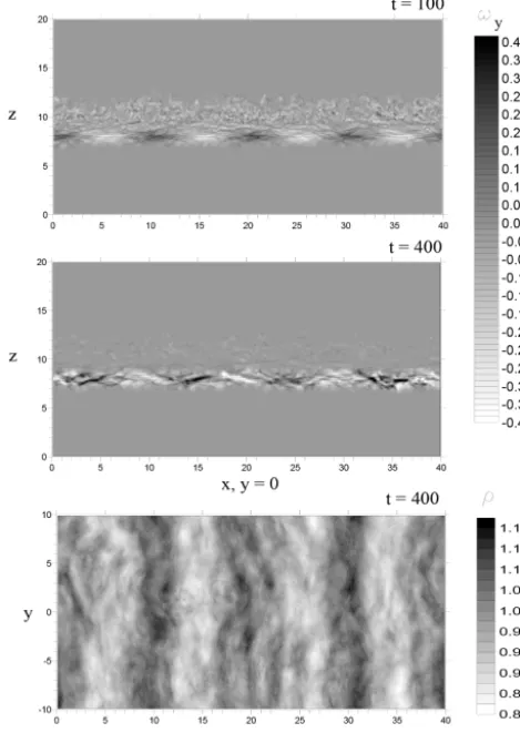
Figure 6. Instantaneous distribution of the vorticityycomponent

ωy(in grey scale) with imposed density contours (1.3, 1.5, 1.7) in

the central (x,z) plane at time momentst=100 andt=400 (top and middle panels, respectively), and density distribution in the (x,

y) plane at the pycnocline level (z=8, bottom panel) att=400 obtained in DNS of the turbulence layer. IW wavelengthλ=10.

ized by distinct maxima and minima in the vicinity of IW troughs and crests, respectively. In the region 9< z <12, the Richardson number is small (Rig<1; cf. Fig. 4) and vortic-ity distribution is similar to that observed in the absence of IW (cf. Fig. 3e). On the other hand, at timet=400 (Fig. 7, middle panel), the vorticity is mostly concentrated in the vicinity of the pycnocline, in a thin layer around the pyc-nocline center at z≈8. Here, Rig>1, and turbulence can be regarded as strongly stratified (cf. Fig. 4). In the upper layer (z >9), the vorticity practically vanishes. Thus, at late times, turbulence is supported by an IW against the effect of the molecular dissipation only in the vicinity of the pycno-cline center, and decays in the upper layer. This observation is also in agreement with the laboratory results by Matusov et al. (1989).

It is of interest to note that a similar enhancement of tur-bulence was observed by Tsai et al. (2015) in the vicinity of the waved water surface. Their DNS results show that

turbu-0.1 1 10 100 1e-010

1e-009 1e-008 1e-007 1e-006 1e-005 0.0001 0.001 0.01

t = 400 turb.with IW, z = 8 IW without turb., z = 8 turb. without IW, z = 9

0.1 1 10 100 k

Ey

k E

Figure 7. The kinetic energy power spectrum,E(k)(left), and the spectrum of they-velocity component,Ey(k)(right), obtained in

DNS with initially excited IWs at the pycnocline center level (z=8) at timet=400. The kinetic energy spectrum of the internal wave in the absence of a turbulent layer and spectraEandEyof turbulence

without an initially induced IW obtained at the level of maximum kinetic energy (z=9) at timet=400 are also provided for compar-ison.

lence is enhanced by the straining field of the surface wave in the vicinity of the water surface, and this enhancement is most pronounced in the vicinity of the surface wave crests and troughs. Since the IW-induced strain field decreases ponentially with the distance from the pycnocline, it is ex-pected that the effect of the IW field on turbulence is most pronounced in the immediate vicinity of the pycnocline, as is observed in our DNS in Fig. 6.

The distribution of the density (ρ+ρref(z))at timet=400 (Fig. 6, bottom panel) shows that IW is significantly distorted by increased turbulence along the front. This refraction of IW under the effect of turbulence can be the source of more sig-nificant IW damping in the case when increasing turbulence amplitude becomes comparable with IW amplitude, as was also observed by Druzhinin et al. (2013).

Figure 7 presents the kinetic energy power spectrum,E, and the spectrum of they-velocity component,Ey, of turbu-lence with an IW (propagating in the pycnocline) obtained in DNS at the pycnocline center level (z=8) at timet=400. The figure also shows the kinetic energy spectrum of the in-ternal wave in the absence of a turbulence layer, and spec-traEandEyof turbulence in the absence of an IW at level z=9 (where turbulence kinetic energy has a local maximum att=400; cf. Fig. 3a).

(11)

left panel). That means that the nonlinearity of IW is small and that the internal wave is far from breaking. The kinetic energy spectrum of turbulence with IW is also characterized by a well-pronounced peak at the first-harmonics wave num-ber (k=2π/10), and the amplitude of this peak practically equals the amplitude of the first-harmonics peak in the IW spectrum without turbulence. That means that, at this wave number (k=2π/10), the direct contribution of IW to the ki-netic energy is most prominent. On the other hand, spectrum E(k) of turbulence with IW is also significantly enhanced (as compared to the turbulence spectrum in the absence of IW) at otherk, where there is no direct contribution of IW to kinetic energy. Note also that since the energy peak at the IW wave numberk=2π/λ=0.628 in the TKE spectrum is most pronounced, the turbulent length scale, in this case, is actually determined by the IW length (λ=10). Then the tur-bulent Reynolds number can be estimated asRet=LtUt0Re

=λUt0Re=20 000 for the amplitudeUt0=0.1.

Comparison of the spectra of the y-velocity component, Ey(k), obtained in DNS with and without IW propagating in the pycnocline (Fig. 7, right panel), shows that the spec-tra coincide at the wave number of the first IW harmonics (k=2π/10), and Ey(k) of turbulence with IW is signifi-cantly enhanced for both lower and higherk. Note that since the IW velocity field consists only ofx andzcomponents, there is no direct contribution of the IW field in theEy(k) spectrum.

6 Conclusions

We have performed DNS of turbulence dynamics in the vicinity of a pycnocline and studied the effect that a monochromatic internal wave propagating along the pycn-ocline incurs on turbulence dynamics.

DNS results show that, if no IW is initially induced in the pycnocline, turbulence decays and the turbulence kinetic en-ergy (TKE) decreases with time. The TKE decay rate is re-duced in the vicinity of the pycnocline. We assume that this reduction of the TKE decay rate can be related to a grow-ing horizontal length scale of turbulent eddies due to the sta-ble stratification effect. At sufficiently late times, most of the turbulent energy is located in a layer close to the pyc-nocline. Here, the local Richardson number (defined by the local buoyancy frequency and TKE dissipation rate) is large (Ri1), and turbulence dynamics is dominated by quasi-two-dimensional large-scale (pancake) vortex structures.

DNS results also show that, under the effect of an internal wave (IW) propagating in the pycnocline, both the mean ki-netic energy of turbulence and the kiki-netic energy spectrum are significantly enhanced (almost by the order of magni-tude) in the vicinity of the pycnocline center as compared to the case of turbulence decaying without initially induced IW. This observation is in qualitative agreement with the results of the laboratory experiment by Matusov et al. (1989).

In conclusion, let us briefly discuss a possible scaling of the above results to typical laboratory and in situ conditions. In the present study, we employ velocity scales, length scales and timescales,U0,L0andT0=L0/U0, to normalize phys-ical variables. Note that since the timescale is defined as T0=1/N0 and the velocity scale as U0=L0/T0=L0N0, the bulk Richardson number in DNS identically equals unity, Ri = N₀2L2₀/U₀2=1. For laboratory conditions, we prescribeL0=20 cm (IW wavelengthλ=2 m, pycnocline thickness 20 cm) and for the considered Reynolds number Re=20 000 and kinematic viscosity ν=0.01 cm2s−1, we obtain U0=Reν/L0=10 cm s−1 for initial turbulence ve-locity and 0.1U0=1 cm s−1for IW vertical velocity ampli-tude; the timescale isT0=2 s and the buoyancy frequency is N0=0.5 rad s−1. Then, extrapolating our results to oceanic conditions, we takeN0=0.01 rad s−1 _{(Phillips, 1977), i.e.,} T0=100 s for the timescale and L0=20 m for the length scale (IW wavelength 200 m, pycnocline thickness 20 m). Thus, the velocity scale isU0=20 cm s−1, and initial turbu-lence velocity and the IW vertical velocity amplitude are both 0.1U0=2 cm s−1. Although the analysis of specific oceanic situations is beyond the framework of this paper, it provides a stricter mathematical confirmation of the early conclusions by Matusov et al. (1989).

Acknowledgements. This work was supported by RFBR (Project

Nos. 14-05-00367, 15-05-02430). Edited by: H. J. Fernando

Reviewed by: I. Esau and S. Sukoriansky

References

Anis, A. and Moum, J. N.: Surface wave-turbulence interactions: scalingε(z) near the sea surface, J. Phys. Oceanogr., 25, 2025– 2045, 1995.

Carruthers, D. J. and Hunt, J. C. R.: Velocity fluctuations near an interface between a turbulent region and a stably stratified layer, J. Fluid Mech., 165, 475–501, 1986.

Druzhinin, O. A., Ostrovsky, L. A., and Zilitinkevich, S. S.: The study of the effect of small-scale turbulence on internal gravity waves propagation in a pycnocline, Nonlin. Processes Geophys., 20, 977–986, doi:10.5194/npg-20-977-2013, 2013.

Fernando, H. J. S.: Turbulent mixing in stratified fluids, Ann. Rev. Fluid Mech., 23, 455–493,1991.

Hazel, P.: Numerical studies of the stability of inviscid stratified shear flows, J. Fluid Mech., 51, 39–61, 1972.

Kantha, L. H.: On generation of internal waves by turbulence in the mixed layer, Dynam. Atmos. Ocean., 3, 39–46, 1979.

Kantha, L. H.: Laboratory experiments on attenuation of internal waves by turbulence in the mixed layer, Trans. 2nd Int. Symp. on Stratified Flows, Irodheim, Norway, IAHB, 731–741, 1980. Matusov, P. A., Ostrovsky, L. A., and Tsimring, L. S.: Amplification

(12)

Ostrovsky, L. A. and Zaborskikh, D. V.: Damping of internal gravity waves by small-scale turbulence, J. Phys. Oceanogr., 26, 388– 397, 1996.

Ostrovsky, L. A., Kazakov, V. I., Matusov, P. A., and Zaborskikh, D. V.: Experimental study of the internal waves damping on small-scale turbulence, J. Phys. Oceanogr., 26, 398–405, 1996. Phillips, O. M.: The dynamics of the upper ocean, 2nd Edn.,

Cam-bridge University Press, CamCam-bridge, 1977.

Praud, O., Fincham, A. M., and Sommeria, J.: Decaying grid tur-bulence in a strongly stratified fluid, J. Fluid Mech., 522, 1–33, 2005.

Thorpe, S. A.: An introduction to ocean turbulence, Cambridge Uni-versity Press, Cambridge, 2007.

Tsai, W., Chen, S., and Lu, G.: Numerical evidence of turbulence generated by non-breaking surface waves, J. Phys. Oceanogr., 45, 174–180, 2015.

Turner, J. S.: Buoyancy effects in fluids, Cambridge Univ. Press, 1973.