https://doi.org/10.5194/amt-10-3175-2017 © Author(s) 2017. This work is distributed under the Creative Commons Attribution 3.0 License.
Target categorization of aerosol and clouds by continuous
multiwavelength-polarization lidar measurements
Holger Baars, Patric Seifert, Ronny Engelmann, and Ulla Wandinger
Leibniz Institute for Tropospheric Research (TROPOS), Permoser Str. 15, 04318 Leipzig, Germany
Correspondence to:Holger Baars ([email protected])
Received: 20 December 2016 – Discussion started: 10 February 2017
Revised: 29 May 2017 – Accepted: 8 June 2017 – Published: 1 September 2017
Abstract. Absolute calibrated signals at 532 and 1064 nm and the depolarization ratio from a multiwavelength lidar are used to categorize primary aerosol but also clouds in high temporal and spatial resolution. Automatically derived par-ticle backscatter coefficient profiles in low temporal resolu-tion (30 min) are applied to calibrate the lidar signals. From these calibrated lidar signals, new atmospheric parameters in temporally high resolution (quasi-particle-backscatter coeffi-cients) are derived. By using thresholds obtained from mul-tiyear, multisite EARLINET (European Aerosol Research Lidar Network) measurements, four aerosol classes (small; large, spherical; large, spherical; mixed, partly non-spherical) and several cloud classes (liquid, ice) are defined. Thus, particles are classified by their physical features (shape and size) instead of by source.
The methodology is applied to 2 months of continu-ous observations (24 h a day, 7 days a week) with the multiwavelength-Raman-polarization lidar PollyXT during the High-Definition Clouds and Precipitation for advanc-ing Climate Prediction (HD(CP)2) Observational Prototype Experiment (HOPE) in spring 2013. Cloudnet equipment was operated continuously directly next to the lidar and is used for comparison. By discussing three 24 h case stud-ies, it is shown that the aerosol discrimination is very fea-sible and informative and gives a good complement to the Cloudnet target categorization. Performing the categoriza-tion for the 2-month data set of the entire HOPE campaign, almost 1 million pixel (5 min×30 m) could be analysed with the newly developed tool. We find that the majority of the aerosol trapped in the planetary boundary layer (PBL) was composed of small particles as expected for a heavily pop-ulated and industrialized area. Large, spherical aerosol was observed mostly at the top of the PBL and close to the
identi-fied cloud bases, indicating the importance of hygroscopic growth of the particles at high relative humidity. Interest-ingly, it is found that on several days non-spherical particles were dispersed from the ground into the atmosphere.
1 Introduction
Aerosol and clouds are important atmospheric players in-fluencing weather and climate. In contrast to long-lived gaseous components in the atmosphere, these components are short lived and feature a strong spatiotemporal variabil-ity. Aerosols act as cloud condensation nuclei and ice nu-cleating particles and are thus one major driver for cloud optical and microphysical properties and precipitation initia-tion. Because aerosol is emitted from various sources and is short-living, several aerosol types with different optical and microphysical properties exist in different heights of the at-mosphere, influencing solar radiation and clouds in different ways. Therefore, the climate effects of aerosol directly and of aerosols on clouds (indirectly) are still very uncertain (IPCC, 2013).
Aerosols and Radiation Explorer; Illingworth et al., 2015) cover the globe but with low temporal and spatial resolu-tion. Thus, high-performance ground-based observations are also needed. Scientific networks such as Cloudnet (Illing-worth et al., 2007) or the ARM (Atmospheric Radiation Mea-surement) Climate Research Facilities (Mather and Voyles, 2013) use different ground-based instruments at the same lo-cation (supersite) to gather as much information as possible in high temporal and spatial (i.e. vertical) resolution but at specific locations only. Cloudnet, for example, uses as min-imum instrumentation a cloud radar, a ceilometer (a simple backscatter lidar), and a microwave radiometer (MWR) to characterize the atmosphere above the supersite. Cloudnet delivers several products, ranging from calibrated measure-ments to microphysical cloud properties. Very well known and widely used is the Cloudnet target categorization (Hogan and O’Connor, 2004), which classifies a series of different particle types in the observed atmospheric column (e.g. liq-uid droplets, ice crystals, aerosols). However, Cloudnet is not able to distinguish different aerosol types in its current state, which is a prerequisite to constrain aerosol–cloud-interaction studies and to improve the estimation of the radiative proper-ties of aerosol.
Active remote sensing with lidar is a key technique for characterizing aerosol and allows capturing the atmospheric state on a vertically resolved basis usually covering the whole troposphere. For an intense characterization of aerosol type and properties, so-called multiwavelength lidars (MWLs) are applied using the synergistic information from different wavelengths, scattering mechanisms, and polarization states of the received light (e.g. Müller et al., 2007).
Optical aerosol properties have been widely investigated by using lidar profiles in low temporal resolution, applying the traditional Raman method (Ansmann et al., 1992b), the Klett–Fernald method (Klett, 1981; Fernald, 1984), and the depolarization method (e.g. Cairo et al., 1999) to determine the intensive properties (Ångström exponent, extinction-to-backscatter (lidar) ratio, particle depolarization ratio) of dif-ferent aerosol types and their mixtures (Müller et al., 2007; Tesche et al., 2011; Ansmann et al., 2011; Burton et al., 2012; Pappalardo et al., 2013; Groß et al., 2013; Giannakaki et al., 2015; Amiridis et al., 2015; Sugimoto et al., 2014; Illing-worth et al., 2015; Baars et al., 2016).
Based on such measurements, classification schemes for aerosol from high-resolution lidar measurements have been developed for space-borne lidars (CALIPSO, Omar et al., 2009; EarthCARE, Illingworth et al., 2015; Groß et al., 2015), airborne High Spectral Resolution Lidar (HSRL) measurements (Burton et al., 2012; Groß et al., 2013), some specific ground-based instruments (ARM, Darwin, Australia, Thorsen et al., 2015), and lidar networks focusing on the determination of mineral dust concentration in Asia (Asian Dust Network, AD-NET; Shimizu et al., 2010; Sugimoto et al., 2014).
Due to recent advances in hardware, small sophisticated ground-based MWLs (e.g. PollyXT lidar systems, Engel-mann et al., 2016), which can run unattended and au-tonomously 24 h a day, 7 days a week (24/7), have been de-veloped and are deployed globally. Motivated by this tech-nical progress, we aimed at developing a stand-alone tool for continuously running multiwavelength-polarization li-dars for a basic categorization of the observed particles (targets) in analogy to the Cloudnet target categorization. With this tool, we want to obtain an estimate of the domi-nant type of backscatterer (molecules, aerosol types, clouds) which then can be used for further intensive studies and to complement the Cloudnet target categorization. For this ap-proach we focus on the derivation of certain key parameters, which are not needed with high accuracy but are sufficient to perform a first estimate of certain particle types in the atmosphere. The basic lidar quantities used are the attenu-ated backscatter coefficients at 532 and 1064 nm (calibrattenu-ated range-corrected lidar signal) and the calibrated volume lin-ear depolarization ratio at 532 nm. These key parameters are highly useful as they are available for many continuously measuring lidar systems worldwide, e.g. the lidars within PollyNET (Baars et al., 2016), AD-NET, and the space-borne lidar CALIPSO. From these lidar parameters, further prod-ucts have been developed to allow a first-guess particle typ-ing.
To develop this tool and demonstrate the feasibility, poten-tial, and limitations of this approach, we have used the unique data set obtained during the High-Definition Clouds and Precipitation for advancing Climate Prediction (HD(CP)2) Observational Prototype Experiment (HOPE; Macke et al., 2016) in western Germany. The MWL PollyXT(Engelmann et al., 2016) and the Cloudnet instruments (cloud radar, ceilometer, MWR) were deployed in the frame of the Leipzig Aerosol and Cloud Remote Observations System (LACROS, Bühl et al., 2013) next to each other at Krauthausen, Ger-many, continuously for 2 months in Spring 2013. PollyXTis a sophisticated, compact, scientific multiwavelength lidar to which the quality-assurance procedures proposed by EAR-LINET (European Aerosol Research Lidar Network; Pap-palardo et al., 2013) are applied. Without such high-quality measurements, a proper aerosol characterization as described in the following is not possible. The collocation of the in-struments makes the derived data set a perfect environment for developing an aerosol classification from MWL while the Cloudnet categorization can be performed in parallel.
automati-cally retrieve optical properties of the observed particles (e.g. D’Amico et al., 2015), and finally even for retrieving micro-physical properties (Müller et al., 2016; Veselovskii et al., 2015) which then may lead to an advanced particle catego-rization (e.g. HETEAC, hybrid end-to-end aerosol classifica-tion model; Wandinger et al., 2016).
The paper is structured as follows: first, the HOPE cam-paign, i.e. location and instrumentation, is briefly introduced in Sect. 2. The methodology to derive quantitative lidar parameters with temporal high resolution is explained in Sect. 3. Next, the new target categorization is introduced and intensively discussed by means of three case study days dur-ing HOPE in Sect. 4. The new methodology was applied on the complete HOPE data set and analysed in Sect. 5. Finally, conclusions are drawn in Sect. 6.
2 HOPE
During the HD(CP)2 Observational Prototype Experiment (HOPE; Macke et al., 2016), the multiwavelength-Raman li-dar PollyXTIfT(Althausen et al., 2009; Engelmann et al., 2016) was deployed at Krauthausen (50.879746◦N, 6.414571◦E, 110 m a.s.l.), near Jülich, western Germany, in April and May 2013 as part of the LACROS facility (Bühl et al., 2013). A detailed description of the campaign together with the pre-vailing meteorological conditions can be found in Macke et al. (2016).
PollyXTIfT (system version labelled “IfT”, compare Engel-mann et al., 2016) is an automatic, portable multiwavelength-polarization Raman lidar with automatic calibration proce-dures of the latest standards which was operated in 24/7 mode during HOPE. The lidar emits pulses of linearly po-larized light at 355, 532, and 1064 nm at a repetition fre-quency of 20 Hz. The receiver has seven channels detecting the elastically backscattered light at the three aforementioned wavelengths, the cross-polarized light at 532 nm, and the vi-brational Raman scattered light at 387, 407, and 607 nm. With PollyXTIfT, aerosol profiles can be obtained with 30 m vertical and 30 s temporal resolution. The full overlap be-tween the laser beam and the receiver field of view is about 1500 m; thus, an overlap correction (Wandinger and Ans-mann, 2002) is applied below this height. The lidar was oper-ated in photon-counting mode. The system is pointed 5◦ off-zenith to prevent the detection of specular reflection by the planar planes of horizontally oriented ice crystals (Hu et al., 2009; Westbrook et al., 2009). A detailed description of the system including a quality assessment can be found in En-gelmann et al. (2016).
Furthermore, a cloud radar, a Doppler wind lidar, a ceilometer, and an AERONET (Aerosol Robotic Network) sun photometer were deployed next to the lidar as part of the LACROS facility. From these instruments, Cloudnet prod-ucts (Illingworth et al., 2007) and AERONET prodprod-ucts (Hol-ben et al., 2001) are available. Because of radar scanning
ex-periments during HOPE in Jülich, Cloudnet products which require vertically pointing measurements are sporadically unavailable for this campaign.
3 Methodology
In modern multiwavelength lidars, a number of different re-ceiving channels are installed to make use of as much infor-mation from the atmosphere as possible (elastic and Raman [inelastic] scattering, change in polarization state of emit-ted light due to scattering, etc.). In this way, high-quality aerosol products are obtained on a vertically resolved basis. However, because of the high background noise, Raman lidar observations during daytime are challenging. Therefore, for continuous (24/7) measurements, we concentrate on the use of channels for elastic backscattering, including depolariza-tion. The key challenge to succeed with automated aerosol retrievals is the calibration of the lidar signals. There are two main tasks necessary before an automated aerosol target cat-egorization can be performed: the calibration of the backscat-ter profiles and the calibration of the depolarization products. 3.1 Calibration of backscatter
The backscatter signal strengthP (number of counted pho-tons per 30 s and 30 m in the case of the lidar system used here) for a certain rangeR at the wavelengthλ can be de-scribed for each channel by
Pλ(R)=CλO λ(R) R2
h
βparλ (R)+βmolλ (R)i
×exp
−2
R Z
0 h
αparλ (r)+αmolλ (r) i
dr
, (1)
with the wavelength-dependent lidar system parameter Cλ
these methods are not applicable. Therefore, we perform an absolute lidar calibration by deriving the lidar system param-eterCλto obtain foremost the attenuated backscatter coeffi-cient.
For the measurements performed during HOPE,Cλ was derived from particle backscatter coefficient profiles, which were automatically computed with the Raman or Klett– Fernald methods at 30 min resolution as described in Baars et al. (2016). From these profiles,Cλ(R)can be calculated by rearranging Eq. (1) to
Cλ(R)= P
λ(R) R2 h
βλ
par(R)+βmolλ (R) i
Oλ(R)
×exp
2
R Z
0 h
αparλ (r)+αmolλ (r)idr
. (2)
The final Cλ is computed as the mean value of a height window of 1000 m above the full overlap height (i.e. 1500 m in the case of PollyXTIfT) and is considered to be height in-dependent. Cλ is valid for the recorded raw resolution of 30 m, 30 s, and repetition rate of 20 Hz of the lidar system used here. For the automatically retrieved particle backscat-ter profiles from the Polly systems, all known instrumental is-sues (e.g. background subtraction) which could cause height-dependent effects were corrected, except for the partial over-lap in the lowermost part of the lidar profile described by
Oλ(R), which is a substantial feature of each lidar system. For that reason and because the particle extinction coeffi-cient derived with the Raman method is only available dur-ing nighttime, we introduced a two-step approach to estimate the particulate transmission needed to solve Eq. (2). First, we calculate the particle extinction coefficient profile derived from the particle backscatter coefficient profile (Raman or Klett – depending on time of day) multiplied with a constant lidar ratio of 55 sr as a good compromise of the lidar ratio values observed during HOPE and at other European con-tinental sites (clean and polluted concon-tinental aerosol, desert dust, and smoke; Mattis et al., 2004; Müller et al., 2007; Groß et al., 2013; Schwarz, 2016; Baars et al., 2016). Second, we assume height-independent extinction below 500 m to ac-count for both the incomplete overlap within the lidar profile and atmospheric variability in the lowermost troposphere. At 500 m, already more than 80 % of the overlap between the laser and the telescope field of view is reached and the ap-plied overlap correction profile can correct the signal with high accuracy up to the full overlap height. Finally, an ex-tinction profile from the surface up to the height of interest is available to calculate the particulate transmission in Eq. (2).
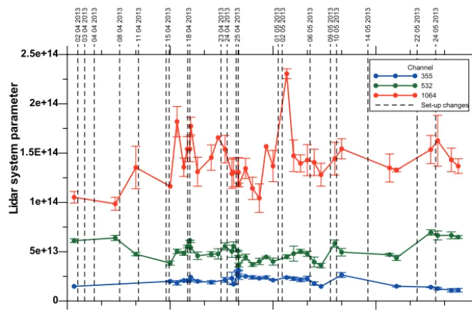
Figure 1 shows the daily mean lidar system parameters calculated as described above for the HOPE campaign. For some days, no calculation was possible due to unfavourable weather conditions and thus the unavailability of automati-cally retrieved backscatter coefficient profiles for calibration.
Vertical dashed lines indicate set-up changes in the lidar. Even though we tried to minimize set-up changes (neutral-density filters, overlap adjustment, laser energy, emission-window cleaning), several changes were necessary but not always influencing the derived lidar system parameter.
One can see that the lidar system parameter is relatively stable and only some of the set-up changes have caused a sig-nificant change inCλ. However, there are also periods were there was a significant change ofCλ even without changes in the set-up, e.g. between 21 April 2013 and 1 May 2013. It was found that changes in the indoor temperature of the cabinet due to air conditioning malfunctioning had led to a change of the alignment (e.g. the overlap between the re-ceiver field of view and the laser beam) and thus a change inCλduring this period. On 2 days (25 April and 10 May), the corresponding data were therefore partly not considered in the analysis. The daily mean lidar system parameter can finally be obtained with an SD (standard deviation) of less than 20 %. The relative change of the lidar system parameter is similar for all three wavelengths, even though it looks dif-ferent in Fig. 1 due to the scaling applied. On 3 days (18, 25 April, and 10 May), for which multiple system set-up changes were performed, more than one lidar system pa-rameter was used to account for these set-up changes. In all other cases, the daily mean system parameter was used when available, otherwise the closest lidar system parameter from the days before or after was applied, to calculate the cali-brated attenuated backscatter coefficient derived by dividing the range-corrected signal with the lidar system parameter:
βattλ(R)=P
λ(R) R2
Cλ =
h
βparλ (R)+βmolλ (R)i
×exp
−2
R Z
0 h
αparλ (r)+αmolλ (r)idr
. (3)
3.2 Calibration of depolarization ratio
The calibration of the depolarization measurements of PollyXT systems is done with the so-called 190◦ -method (Freudenthaler, 2016) in agreement with EAR-LINET standards. For this purpose, a motorized filter wheel is implemented in the receiver unit of PollyXTto perform the
lidar-system-01 04 2lidar-system-013 16 04 2013 01 05 2013 16 05 2013 31 05 2013 0 5e+13 1e+14 1.5E+14 2e+14 2.5e+14 Li dar system parameter 02 0 4 20 13 03 0 4 20 13 08 0 4 20 13 23 0 4 2 01 3 24 0 4 2 01 3 25 0 4 2 01 3 01 0 5 2 01 3 04 0 4 20 13 11 0 4 20 13 15 0 4 20 13 18 0 4 2 01 3 02 05 20 13 06 0 5 2 01 3 09 0 5 2 01 3 10 0 5 2 01 3 14 0 5 2 01 3 22 0 5 20 13 24 0 5 2 01 3 Channel 355 532 1064 Set- up changes
Figure 1.Lidar system parameterCλfor 355, 532, and 1064 nm.Cλis given for the photon counts of the recorded raw resolution of 30 m, 30 s, and repetition rate of 20 Hz corrected for the range dependency (R2) in metres. Vertical lines indicate lidar set-up changes.
01 04 2013 16 04 2013 01 05 2013 16 05 2013 31 05 2013
0 0.1 0.2 0.3
V*
Figure 2.Daily depolarization calibration factorV∗as derived during HOPE.
dependent transmission ratiosDcandDtot(see Engelmann
et al., 2016) of the cross and total channel, respectively, the volume linear depolarization ratio is derived without any fur-ther assumptions by
δvolλ (R)= V
∗−δλ(R) δλ(R)D
tot−V∗Dc
(4) with
δλ(R)= P λ
c(R)
Ptotλ(R), (5)
wherePcλandλPtotare the cross-polarized and total lidar
sig-nals, respectively. In the case of HOPE, depolarization mea-surements are available atλ=532 nm.
3.3 Aerosol characterization
The methodology to derive the lidar system parameters was based on 30 min averaged profiles of the particle backscatter
coefficient, which are only available for specific atmospheric conditions. For the target characterization aimed at in this paper, 24 h measurements with 5 min resolution are analysed to characterize aerosols and clouds. The received signals of the backscattered light at 532 and 1064 nm and the depolar-ization ratio at 532 nm are used for this purpose. In the fol-lowing, the methodology is introduced and then explained in detail in terms of a case study from HOPE.
3.3.1 Obtaining aerosol products – extensive properties
re-duces Eq. (3) to
quasi*βλ
par(R)=β λ att(R)exp
2 R Z 0
αmolλ (r)dr
−βmolλ (R) . (6)
To account for the incomplete overlap of the lidar system in lower heights, an overlap correction function is applied and height-independent backscattering below 500 m is as-sumed in analogy to the calculation of the lidar system pa-rameterCλ. The particle extinction coefficient is now esti-mated in analogy to the procedure during the calculation of
Cλby multiplyingquasi*βparλ (R)with a constant lidar ratio of
Spar=55 sr: quasiαλ
par(r)=quasi*βparλ (R) Spar. (7)
As explained already in Sect. 3.1, the lidar ratio value used serves as a good compromise for lidar ratio values ob-served during HOPE and at other European continental sites. Finally, temporally high-resolved profiles of the so-called quasi-particle-backscatter coefficient defined as
quasiβλ
par(R)=βattλ (R)
×exp 2 R Z 0 h
αmolλ (r)+quasiαparλ (r)idr
−βmolλ (R)
≈βparλ (R) (8)
can be calculated, which serve as best estimate for the parti-cle backscatter coefficientβparλ (R)determined with the Ra-man or Klett method as demonstrated in Sect. 3.3.3. The quasi-particle-backscatter coefficient at 532 and 1064 nm is then used as the input for the particle characterization de-scribed below. An iterative approach for the determination of the particle extinction coefficient using the formulas above is not possible, because the solutions do not converge if the input lidar ratio is not exactly identical to the lidar ratio valid for the observed scatterers. If the input lidar ratio is higher than the atmospheric one, the extinction coefficient and thus also the backscatter coefficient is, in general, overestimated, and the procedure quickly approaches unstable solutions. On the other hand, if the lidar ratio input is too low, too small values that do not increase during the procedure are obtained. This behaviour is similar to the so-called Klett–Fernald for-ward iteration (Klett, 1981; Fernald, 1984), which also relies on a priori information of the lidar ratio and can be numeri-cally unstable.
3.3.2 Obtaining aerosol products – intensive properties With the calibration methods described above, a rough but temporally high-resolved aerosol characterization can be done by using the quasi-particle-backscatter coefficients and the volume depolarization ratio to obtain intensive aerosol-type specific quantities. From the quasi-particle-backscatter
coefficients, the quasi-particle Ångström exponent
quasiåλ1/λ2
par = −
ln
quasi βparλ1
quasiβλ2 par
lnλ1 λ2
(9)
is calculated for the wavelength pairλ1andλ2, e.g. 532 and
1064 nm, to obtain information on particle size. The quasi-particle depolarization ratio defined as
quasiδλ
par(R)=
δλvol(R)+1
× β
λ
mol(R)
δmolλ −δλvol(R)
quasiβλ
par(R)
1+δmolλ +1
!−1
−1 (10)
is also an intensive property and used to obtain information about the particle shape. The molecular depolarization ratio
δmolλ is calculated theoretically from the bandwidth of the in-terference filters (e.g. see Behrendt and Nakamura, 2002) and is 0.0053 at 532 nm in the case of PollyXT(Engelmann et al., 2016).
3.3.3 Example observation: 22 April 2013
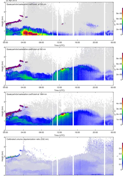
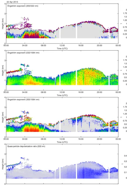
To demonstrate the introduced quantities, the time-height cross sections of the four possible extensive (Fig. 3) and four possible intensive (Fig. 4) particle quantities of PollyXTIfT are shown for 1 day of HOPE – the 22 April 2013.
HOPE, Krauthausen, lidar POLLY XT 22 Apr 2013
0 2e−06 4e−06 6e−06 8e−06
sr
−1 m
−1
0 2e−06 4e−06 6e−06 8e−06
sr
m
−1
−1
0 1e−06 2e−06 3e−06 4e−06
sr
m
−1
−1
0 0.1 0.2 0.3 0.4
1
00:00 04:00 08:00 12:00 16:00 20:00 00:00
Time (UTC) 0
1 2 3 4
Height (km
)
00:00 04:00 08:00 12:00 16:00 20:00 00:00
Time (UTC) 0
1 2 3 4
Height (km
)
00:00 04:00 08:00 12:00 16:00 20:00 00:00
Time (UTC) 0
1 2 3 4
Height (km
)
00:00 04:00 08:00 12:00 16:00 20:00 00:00
Time (UTC) 0
1 2 3 4
Height (km
)
Quasi- particle backscatter coef f icient at 355 nm
Quasi- particle backscatter coeff ficient at 532 nm
Quasi- particle backscatter coe cient at 1064 nm
Calibrated volume depolarization ratio (532 nm) ffi
HOPE. Krauthausen, lidar POLLY XT 22 Apr 2013
0 0.25 0.5 0.75 1 1.25 1.5 1.75 2
1
0 0.25 0.5 0.75 1 1.25 1.5 1.75 2
1
0 0.25 0.5 0.75 1 1.25 1.5 1.75 2
1
0 0.1 0.2 0.3 0.4
1
00:00 04:00 08:00 12:00 16:00 20:00 00:00
Time (UTC) 0
1 2 3 4
Height (km
)
00:00 04:00 08:00 12:00 16:00 20:00 00:00
Time (UTC) 0
1 2 3 4
Height (km
)
00:00 04:00 08:00 12:00 16:00 20:00 00:00
Time (UTC) 0
1 2 3 4
Height (km
)
00:00 04:00 08:00 12:00 16:00 20:00 00:00
Time (UTC) 0
1 2 3 4
Height (km
)
Ångström exponent (355/532 nm)
Ångström exponent (532/1064 nm)
Ångström exponent (355/1064 nm)
Quasi- particle depolarization ratio (532 nm)
The quasi-particle depolarization ratio is also enhanced at the lower cloud boundaries due to multiple scattering and/or because of falling ice crystals. The three quasi-particle Ångström exponents (Fig. 4) exhibit a very different be-haviour showing that the Ångström exponents incorporat-ing the quasi-particle-backscatter coefficient at 355 nm are not representative. This is due to the corrections and as-sumptions made to estimate the particulate extinction and fi-nally the quasi-particle-backscatter coefficient. As at 355 nm molecular backscattering is 80 (5) times higher than at 1064 (532) nm, large uncertainties are introduced into the at-tenuation correction presented in Sect. 3.3.1 when 355 nm signals are considered, even though the lidar system param-eter is known with good accuracy. The partial negligence of particulate extinction in the first-guess profile (Eq. 6) and the subtraction of the molecular scattering contribution leads of-ten to very large errors (as molecular backscattering is usu-ally much stronger than particle backscattering at this wave-length) with even negative quasi-particle-backscatter coeffi-cients. These effects are illustrated in Fig. 5 for a 30 min pe-riod of 22 April 2013. The particle backscatter coefficients determined with the Klett method, the attenuated backscatter coefficients, and the quasi-particle-backscatter coefficients are shown for the different wavelengths.
We have also considered other approaches to estimate the extinction at 355 nm for the calculation of the quasi-particle-backscatter coefficient (cp. Eq. 8), for example, by using the Ångström relationship (Ångström, 1964) to convert the 1064 nm extinction with an assumed a priori extinction-related Ångström exponent to the extinction coefficient pro-file at 355 nm similar to Eq. (9). Three different Ångström exponents were chosen which are representative for the HOPE campaign, i.e. 1.0, 1.4, and 2.0, to obtain the extinc-tion at lower wavelengths from the extincextinc-tion at 1064 nm. This procedure is illustrated also in Fig. 5, where addition-ally the three backscatter coefficient profiles derived with this methodology are plotted. However, with that approach it was also found that the a priori choice of the extinction-related Ångström exponent is so crucial at 355 nm that it cannot be applied in an automatic retrieval (e.g. see profile derived with an Ångström exponent of 2.0 at 355 nm). Closest to the par-ticle backscatter coefficient at all wavelengths is the quasi-particle-backscatter coefficient derived with the methodol-ogy described in Sect. 3.3.1 (without the Ångström exponent assumption for extinction estimation). Taking into account the satisfying results at 1064 and 532 nm with this approach, one can conclude that the quasi-particle-backscatter coeffi-cient is a better estimate than the attenuated backscatter co-efficient for particle backscattering in the atmosphere.
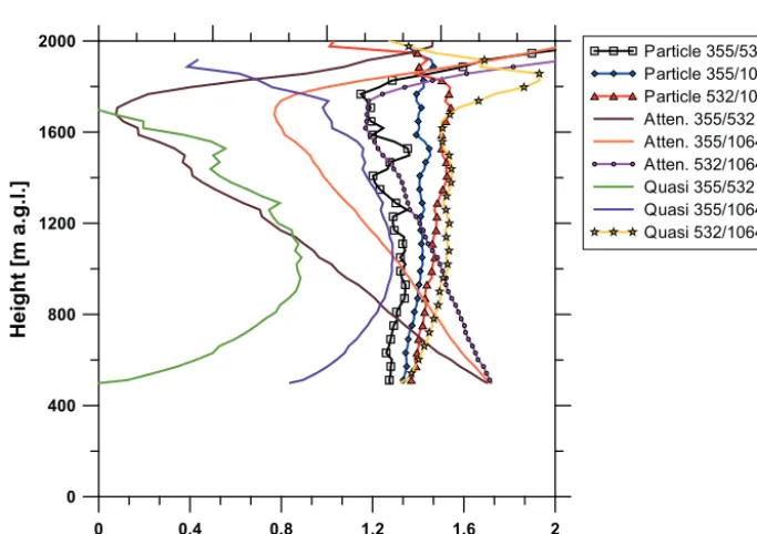
This finding is also proved when comparing the different Ångström exponents as done in Fig. 6. Here, the Ångström exponents derived from the quasi-particle-backscatter coeffi-cients at 532 and 1064 nm (deep yellow with stars) are very similar to the ones obtained from the particle backscatter co-efficients derived with the Klett method (black, blue, and red,
all close to 1.4 and height independent for the aerosol layer up to 2 km). However, the Ångström exponents using the 355 nm quasi-particle-backscatter coefficients show already significant deviations (avocado green and purple) from the aforementioned value of 1.4. Even worse are the results when the attenuated backscatter coefficients are used (dark brown, orange, and magenta with circles), which shows again that this quantity cannot be applied for particle typing by using multiple wavelengths.
Consequently, we apply the quasi-particle-backscatter co-efficients at 532 and 1064 nm, which are straightforward to determine and which are close to the atmospheric truth; the corresponding quasi-particle Ångström exponent; and the quasi-particle depolarization ratio at 532 nm for the tempo-rally high-resolution target categorization.
4 Typing
For the typing of atmospheric features, i.e. the optical dominant scatterer type, three extensive (quasi-particle-backscatter coefficient at 532 and 1064 nm and volume depo-larization ratio) and two intensive properties (quasi-particle Ångström exponent and quasi-particle depolarization ratio) are available to detect aerosol and cloud layers and to dis-tinguish between those two and classify subtypes. The lidar-only attempt is made to categorize aerosols and clouds con-cerning different types in analogy to the Cloudnet classifi-cation. In the following, the methodology is described fol-lowed by an intensive discussion concerning the applicability by means of example cases of HOPE.
4.1 Typing methodology
Rl eal A tten. Q uasi Å=1.0 1.4 2.0
0 5e-6 1e-5 1.5e-5 2e-5
Backscatter coefficient [m-1 sr-1] 0
1000 2000 3000 4000
H
ei
gh
t [
m
a
.g
.l.
]
355 nm
R eal A tten. Q uasi 1.0 1.4 2.0
2e-6 4e-6 6e-6
Backscatter coefficient [m-1 sr-1]
532 nm
R eal A tten. Q uasi
5e-7 1e-6 1.5e-6 2e-6
Backscatter coefficient [m-1 sr-1]
1064 nm
0 0
Å= Å=
Å= Å= Å=
Figure 5.Comparison of the particle backscatter coefficient determined with the Klett method, the attenuated backscatter coefficient, and particle-backscatter coefficient for the three laser emission wavelengths on 22 April 2013, 14:20–14:50 UTC. Additionally, the quasi-particle-backscatter coefficient with a different approach for attenuation correction (extinction coefficient derived from the 1064 nm extinction coefficient with the Ångström relation) is plotted for Ångström exponents of Å=1.0, 1.4, and 2.0
0 0.4 0.8 1.2 1.6 2
Ångström exponent
0 400 800 1200 1600 2000
H
ei
gh
t [
m
a
.g
.l.]
P article 355/532 P article 355/1064 P article 532/1064 A tten. 355/532 A tten. 355/1064 A tten. 532/1064 Q uasi 355/532 Q uasi 355/1064 Q uasi 532/1064
Figure 6. Comparison of Ångström exponents derived from the particle backscatter coefficients determined with the Klett method, the attenuated backscatter coefficients, and the quasi-particle-backscatter coefficients for 22 April 2013, 14:20–14:50 UTC. A five-bin vertical smoothing was applied.
Optical thick clouds are identified using the Cloudnet scheme for droplet finding (Illingworth et al., 2007; Hogan and O’Connor, 2004). As the lidar cannot penetrate liquid clouds, we cannot detect the cloud top, in contrast to Cloud-net, which uses the cloud radar information to gather this value. Therefore, the lidar target categorization will detect the cloud base and hydrometeors some tens of metres above the base. In principle within this scheme, clouds are de-tected if the quasi-particle-backscatter coefficient at 1064 nm
is higher than 2×10⁻⁵m−1sr−1and the signal decreases by
A�en. bsc at 355 nm valid
Molecular
sca�ering
Quasi-bsc at 1064 nm > 1e-8 m sr-1 -1
Quasi-bsc at 1064 nm > 2e-7 m sr-1 -1
Cloud typing Aerosol typing aerosol/low Non-typed
concentra�on Cloudnet cloud iden�fica�on
Ice cloud typing
No signal
S mall L arge Mixture spherical
Non-typed dropsL ikely D rops
Ice
L ikely ice
Figure 7.Schematic illustration of the typing procedure. Details in text and Table 1.
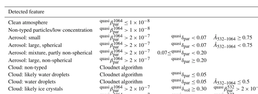
Table 1. Overview of particle typing. Criteria for the feature classes are given. Quasi-particle-backscatter coefficient values are given in m−1sr−1.
Detected feature
Clean atmosphere quasiβ1064par ≤1×10⁻⁸ Non-typed particles/low concentration quasiβ1064par >1×10⁻⁸
Aerosol: small quasiβ1064par >2×10⁻⁷ quasiδpar<0.07 Å532–1064≥0.75
Aerosol: large, spherical quasiβ1064par >2×10⁻⁷ quasiδpar<0.07 Å532–1064<0.75
Aerosol: mixture, partly non-spherical quasiβ1064par >2×10⁻⁷ 0.07≤quasiδpar<0.20
Aerosol: large, non-spherical quasiβ1064par >2×10⁻⁷ quasiδpar≥0.20
Cloud: non-typed Cloudnet algorithm
Cloud: likely water droplets Cloudnet algorithm quasiδpar≤0.05
Cloud: water droplets Cloudnet algorithm quasiδpar≤0.05 Å532–1064≤0.5
Cloud: likely ice crystals quasiβ1064par >2×10⁻⁷ quasiδvol≥0.30 quasiβpar532>2×10⁻⁷
Cloud: ice crystals quasiβ1064par >2×10⁻⁷ quasiδpar≥0.35 quasiβpar532>2×10⁻⁷
2×10⁻⁵m−1sr−1accounts for an extinction coefficient of about 3.6×10⁻⁴m−1at all wavelengths (lidar ratio of 18 sr for water droplets, Ångström exponent of 0 for large parti-cles). According to the OPAC database (Hess et al., 1998), an extinction coefficient value of 3.6×10⁻⁴m−1is higher
than the values at 550 nm given for all aerosol types ex-cept for strong pollution. According to Liu et al. (2009), a threshold of 1×10⁻⁵m−1sr−1 at 1064 nm is well suited for the discrimination between cloud and aerosol because the largest overlap between the two types is between 4×10⁻⁶ and 1×10⁻⁵m−1sr−1. The automatically retrieved particle backscatter coefficient profiles as presented in Baars et al. (2016) showed that during HOPE aerosol particle backscat-ter coefficients did not exceed 1×10⁻⁵m−1sr−1(95 %
per-centile maximum at 3×10⁻⁶). Thus, we consider the chosen threshold as valid for the conditions during HOPE without overlapping of the categories. Visual inspection showed no misclassification of liquid clouds, which convinces us that the approach is valid for the detection of cloud bases. As soon as a liquid or non-typed cloud is classified, no other classes above are evaluated because of the risk of strong at-tenuation, multiple scattering, etc., which disturb the signals significantly as the lidar applied is designed for aerosol and not for cloud detection.
We classify the atmosphere as clean if the quasi-particle-backscatter coefficient at 1064 nm is less than 1×
of 30 s) is present. This threshold yields a ratio of molec-ular to particle backscattering at 532 (355) nm higher than 60 (180) at sea level and thus is valid for a Rayleigh calibra-tion by means of the Raman or Klett–Fernald lidar method. One future application of the target categorization presented herein might be to find appropriate regions for Rayleigh cal-ibration, i.e. height regions of almost pure molecular scatter-ing and sufficiently high SNR.
The threshold of 1×10⁻⁸m−1sr−1is also well below the given range for aerosols according to Winker et al. (2009) for the CALIPSO classification. As the PollyXTsystems have a higher detection sensitivity than CALIPSO, we cannot con-sider a higher threshold for clean atmosphere with Rayleigh scattering only. Anything above this threshold is first classi-fied as non-typed particles, which could be aerosol or clouds. Aerosol and ice clouds are typed for a quasi-particle-backscatter coefficient at 1064 nm greater than 2×
10−7m−1sr−1. Everything below remains classified as
“non-typed particles/low concentration”. The threshold is equiv-alent to the one used in the CALIPSO feature mask (5×
10−7m−1sr−1 for the 532 nm attenuated backscatter coef-ficient, Omar et al., 2009) when considering an Ångström exponent of 1.4 as measured by AERONET on average dur-ing HOPE.
If the quasi-particle depolarization ratio is less than 0.07 and the quasi-particle Ångström exponent ≥0.75, the scat-terers are considered to be small particles. If the Ångström exponent is lower, it is supposed that large particles domi-nate the optical properties in the atmospheric volume. A mix-ture of non-spherical and spherical particles is considered when the particle depolarization ratio is between 0.07 and 0.2, while above 0.2 the particles are categorized as large and non-spherical. The thresholds for the aerosol typing are chosen according to Amiridis et al. (2015) and Schwarz (2016), whose analyses of observations at several EAR-LINET stations show that large particles (marine, dust) have an Ångström exponent (532–1064 nm) less than 0.75 while smaller particle types (smoke, polluted continental, etc.) have an Ångström exponent (532–1064 nm) larger than 0.75. Pure Saharan dust is supposed to have a particle depolarization ra-tio at 532 nm of 31 % (Tesche et al., 2009b; Ansmann et al., 2011), but lower ratios were also observed (e.g. around 28 %; Baars et al., 2016). Therefore, we consider particle depolar-ization ratios higher than 20 % as mostly containing dust (or other non-spherical particles) and thus classify the scatterers as large, non-spherical particles. According to Tesche et al. (2009a), a 20 % particle depolarization ratio corresponds to a dust fraction in terms of backscattering of more than two-thirds. A particle depolarization ratio of 7 %, on the other hand, corresponds to a dust fraction of less than 20 %.
In contrast to other classification schemes (e.g. CALIPSO, Omar et al., 2009; HSRL, Burton et al., 2012), we do not cat-egorize by aerosol origin (e.g. mineral dust, biomass burning smoke, etc.), but by physical features. For example, large, non-spherical particles are in most cases mineral dust
ad-vected to the site but could also be volcanic ash, pollen, or local dust plumes. The interpretation is not possible without additional information and thus will be left to the user of the categorization. We want to focus on the physical properties as these are the quantities we can obtain with this lidar-only approach.
Ice crystals, as they occur in cirrus clouds or virgae, are identified by their highly depolarizing properties indepen-dent of the cloud iindepen-dentification or the aerosol typing and thus may overwrite these classes. As cirrus may be optically very thin, the same backscatter coefficient threshold as for aerosol is used to find ice crystals. The class “likely ice” is identified if the volume depolarization ratio (independent of quasi-particle-backscatter coefficient) is higher than 30 %. “Ice crystals” are identified if the particle depolarization ra-tio is higher than 35 % and may overwrite the “likely ice” class. However, the identification of ice crystals is the most critical matter, as sometimes the depolarization information at 532 nm is not available due to the low SNR, whereas with the 1064 nm channel these particles can be detected. Thus, many ice crystals remain unclassified and are categorized as non-typed particles or clouds.
In the next section, we want to demonstrate the perfor-mance of the newly developed target categorization by means of three example cases.
4.2 Examples for the aerosol categorization
In the following, the observation days of 22, 4, and 18 April during HOPE are discussed by means of the lidar target cat-egorization. These example cases represent a wide variety of different meteorological situations and are therefore well suited to demonstrate the capabilities of the newly developed lidar target categorization.
4.2.1 22 April 2013
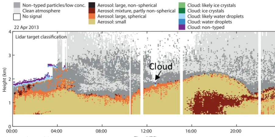
Figure 8.Lidar particle categorization for 22 April 2013.
cloud deck dissolved, and an aerosol layer with mostly small particles but large particles at the top remained the whole day. In addition, a small cumulus cloud was observed shortly past 12:00 UTC at the top of the convective PBL, remaining the only cloud at daytime on this day. The aerosol layer top and thus also the PBL top reached its maximum with 2.2 km at around 19:00 UTC before the aerosol layer starts to decay. We have to note that from the lidar target categorization the identification of the PBL, i.e. the mixing layer height, is not possible and needs additional information; therefore, we re-fer with the term PBL to the main aerosol layer which might have very often coincided with the mixing layer during day-time.
An interesting feature is the entrainment of partly non-spherical particles (brown) between 16:00 and 19:00 UTC from the surface. After 19:00 UTC, these non-spherical par-ticles were detected close to the top of the nocturnal aerosol layer. The source of these non-spherical particles could be lo-cal dust (from open-pit mining close by, see Fig. 2 in Macke et al., 2016) and/or pollen from the local agricultural activ-ity (e.g. see Fig. 1b in Maurer et al., 2016). Such entrainment from ground was very often observed in April at Krauthausen and needs to be investigated further in the future. Above the main aerosol layer, some aerosol, but in low concentration, is identified (dark grey), which means that these regions are not suitable for the so-called Rayleigh fit (Freudenthaler, 2009) needed for the Raman or Klett–Fernald lidar method for which one needs regions of molecular scattering only (light grey).
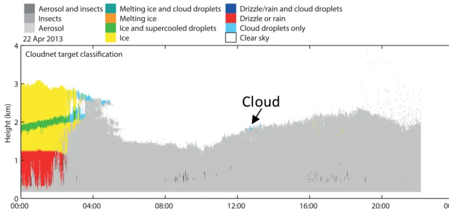
For comparison, Fig. 9 shows the standard Cloudnet clas-sification (Illingworth et al., 2007) which is derived from cloud radar, microwave radiometer, and ceilometer
obser-vations. This classification allows us to distinguish between the different cloud types and to detect aerosol. However, no discrimination between aerosol types is possible. At around 2 km between 00:00 and 03:00 UTC, a supercooled liquid layer was clearly observed (slightly above the lidar-detected cloud base). Below, ice crystals were identified, which turned into liquid at about 1.2 km. According to temperature pro-files retrieved from GDAS11 for the lidar location, the 0◦C altitude was 1.4 km, confirming the findings. The identifica-tion of the liquid droplet layer by Cloudnet shows that the detected cloud features by lidar are certainly mostly liquid droplets and thus confirm the correct classification by the li-dar categorization. The lili-dar, however, did not identify drops or ice below the cloud, most probably due to the low con-centration of these hydrometeors for which the lidar is not sensitive. After 04:00 UTC, Cloudnet classifies aerosol only. The small cloud layer as observed with the MWL is also de-tected shortly past 12:00 UTC.
Finally, we can conclude the lidar-only target categoriza-tion works well and is in agreement with Cloudnet even though the different instrumentations allow the detection of different atmospheric features as intensively discussed in the next case study.
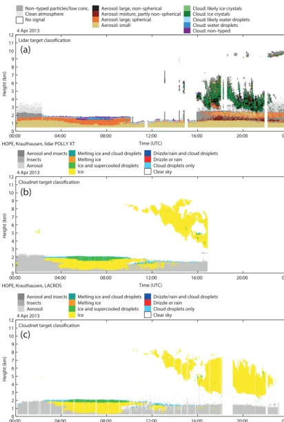
4.2.2 4 April 2013
A second example case to be discussed is 4 April 2013 at Krauthausen. The MWL target classification (top) and the Cloudnet ones (centre and bottom: LACROS and JOYCE) are shown in Fig. 10. JOYCE (Jülich ObservatorY for Cloud
1Global Data Assimilation System, https://www.ready.noaa.
Figure 9.Cloudnet target categorization for 22 April 2013.
Evolution; 3 km away) data are shown because no data from Cloudnet are available for LACROS past 17:00 UTC due to maintenance work on the cloud radar. Nevertheless, the most interesting feature on this day is the overcast cloud condi-tion between 03:00 and 10:00 UTC. During this time, the MWL classification detects very well the cloud base (cloud or likely cloud) and large aerosol below. The Cloudnet clas-sification, however, detects the liquid cloud base as well, but it classifies below ice and super cooled droplets and/or ice not touching the ground. According to the temperature pro-file derived from the GDAS1 data set, a strong inversion was present between 1.8 and 2.2 km and temperatures were below 0◦C throughout the troposphere. Thus, both classifications are reasonable, and one could suppose that the ice and driz-zle detected by the radar led to evaporation which increased the relative humidity (RH) in the aerosol layer and led to hy-groscopic growth and finally, as detected, to large, spherical aerosol particles. As at the cloud base 100 % RH can be con-sidered, the particles just below the cloud experienced high RH, and thus a strong particle growth has most likely led to increased scattering (e.g. Skupin et al., 2014).
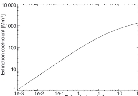
This example shows the different sensitivity concerning particle size and thus the potential synergy between the lidar-and radar-based classifications. While the lidar is more sensi-tive to the numerous but comparably small aerosol particles, the radar is most sensitive to the few but large precipitation particles. If we assume a Marshall–Palmer rain droplet num-ber size distribution (Marshall and Palmer, 1948), we can es-timate the light extinction of the drizzle in dependence of the rain rate as shown in Fig. 11. For low rain rates, which have occurred in the case of 4 April 2013 because no precipitation reached the ground, extinction coefficients well below typ-ical aerosol values are calculated. Aerosol extinction in the
PBL was about 150 to 200 Mm−1 throughout the observa-tion time in the case presented here. At a height of 1.5 km, which is 250 m below the cloud base, extinction coefficients of about 100 Mm−1were observed at 04:00 UTC. When no clouds were present at 01:00 UTC, they were 35 to 50 Mm−1 at this height. Thus, if one considers hygroscopic growth, one can conclude that the lidar signal was dominated by aerosol instead of the few drizzle droplets even though they also con-tributed to the lidar return. On the other hand, as the radar is sensitive to the sixth power of the diameter of the scatterers (while the lidar is to the power of 2), it is sensitive to the few but large precipitation droplets. Therefore, the Cloudnet classification defines the region of interest to contain ice and supercooled drops and ice only – putting the priority on the cloud-sensitive radar observations. Given the added value of the multiwavelength lidar aerosol classification, we can how-ever conclude that between 03:00 and 10:00 UTC all detected features, i.e. large, spherical aerosol particles and ice and su-percooled drops, were present simultaneously, even though the full instrument synergy of the instruments presented here is still a current research topic.
Past 11:00 UTC, another cloud with its base at around 1 km was detected at the top of the growing PBL. Again, the cloud base is identified with lidar at the height at which Cloudnet identifies cloud droplets only. Above and below the cloud base, Cloudnet classifies ice crystals, which cannot be verified with the MWL target categorization. There, mostly small, but also some large, spherical particles close to the cloud base are identified. Above the cloud base, no valid li-dar signal is available.
1e-3 1e-2 1e-1 1 1 10 100
Rain rate [mmh–1]
1 10 100 1000 10 000
E
x
ti
n
ct
io
n
c
o
e
ffi
ci
e
n
t
[M
m
-1]
Figure 11.Simulated light extinction coefficient for drizzle in de-pendence of rain rate.
before at altitudes up to 9 km, which is not possible with the MWL during the low-level-cloud-deck period. Interestingly, during the period past 16:00 UTC, a lofted aerosol layer was found below the ice cloud between 2 and 3 km classified mostly as spherical particles. Below, in the transition zone to the PBL, non-spherical particles were identified because of an increased depolarization ratio. In the PBL itself, small, spherical particles were observed. The Cloudnet observations from JOYCE only 3 km away, however, gave no indication of ice crystals at this altitude, so we can conclude that the non-spherical particles were advected towards the site.
Interestingly, at around 17:00 UTC, large, spherical par-ticles are directly classified below/within the ice cloud at around 3.5 km because of low depolarization values. We can only speculate that due to evaporation of ice crystals, resid-ual aerosol might have grown. Unfortunately, the radar at LACROS was not in operation to investigate this feature in more detail.
As can be seen as well in Fig. 10a, ice crystals are of-ten classified correctly but sometimes remain unclassified or are even falsely classified as aerosol. The reason for the non-classification of ice crystals is mostly the lack of depolar-ization information at 532 nm while the 1064 nm channel is able to detect particles especially at high altitudes at which the SNR of the 532 nm channels is too low. This occurs, e.g. for the thin ice cloud at about 10 km past 21:30 UTC.
The frequency of occurrence of misclassification of ice crystals as aerosol is increasing with increasing penetration depth of the ice clouds as can be seen in Fig. 10a past 16:00 UTC in the height range of 4–7 km. The reason for that false classification is the used a priori information aiming on aerosol (i.e. the lidar ratio and Ångström exponent). This leads to a wrong attenuation correction and thus to wrong quasi-particle-backscatter coefficient and quasi-particle de-polarization ratio values above the cloud base. Furthermore, multiple scattering at the large cloud hydrometeors leads to an additional underestimation of the light attenuation (see
Seifert et al., 2007; Kienast-Sjögren et al., 2016, or Gouveia et al., 2017). For that reason, the current lidar stand-alone ap-proach is trustworthy only at cloud bases and a few tens of metres above, depending on the cloud optical thickness. Nev-ertheless, in the case of ice clouds, the classification is also performed above the cloud base as the cloud optical thick-ness is usually low and thus false classification is compara-bly rare, as seen in Fig. 10a. However, we think the cloud classification can be significantly improved, when the lidar-only categorization is combined with the Cloudnet one, as explained in the outlook, because the use of cloud radar in-formation will allow setting different a priori inin-formation for the clouds.
This case study also shows that, under conditions of low-level clouds, atmospheric features can be identified by MWL with the newly developed methodology, which is not easily possible with the traditional Raman or Klett–Fernald lidar methods.
4.2.3 18 April 2013
The third example day, 18 April 2013, is shown in Fig. 12. This day is characterized by strong westerly winds with wind gusts up to 16 m s−1 as it was found from Doppler li-dar observations. On this day, a mixture with non-spherical aerosol in the lowermost boundary layer was observed al-most continuously, except for the period of cloud occurrence between 05:00 and 07:00 UTC. This liquid cloud is identi-fied with MWL and Cloudnet in good agreement. The MWL classification detects an optically thin lofted aerosol layer between 2 and 3.5 km height after the low cloud layer dis-appeared at around 07:00 UTC. Cloudnet did not detect this aerosol layer. At the top of this layer, a cloud formed shortly past 08:00 UTC. Both clouds are identified to be pure liquid by both algorithms. Shallow boundary layer clouds were ob-served occasionally past 12:00 UTC.
Due to the strong westerly winds, we conclude that the observed non-spherical particles in the PBL originate from the open-pit mine of Inden (see Fig. 2 in Macke et al., 2016) west of our measurement location. Most of these particles re-mained below 1 km at the lidar site (except during the grow-ing phase of the PBL from 10:00 to 12:00 UTC). This is an indication that the particles were just entrained into the PBL and had not had the time to be transported to the top of the PBL yet. Another reason could be that the particles were of much larger size than typical aeolian dust and thus sediment much more rapidly after their emission than other particle types. Visual inspection of the pit mine of Inden, 1.5 km west of the LACROS site, proved strong dust emissions as shown in Fig. 13.
18 Apr 2013
4 Cloud: non−typed
Cloud: water droplets Cloud: likely water droplets Cloud: ice crystals Cloud: likely ice crystals
Aerosol: small
Aerosol: large, spherical
Aerosol: mixture, partly non−spherical Aerosol: large, non−spherical
No signal Clean atmosphere
Non−typed particles/low conc.
HOPE, Krauthausen, lidar POLLY XT
00:00 04:00 08:00 12:00 16:00 20:00 00:00
Time (UTC) 0
1 2 3
Height (km
)
Lidar target classification
18 Apr 2013 Aerosol Insects
Aerosol & insects
Ice
Ice & supercooled droplets Melting ice
Melting ice & cloud droplets
Clear sky
Cloud droplets only Drizzle or rain
Drizzle/rain & cloud droplets
00:00 04:00 08:00 12:00 16:00 20:00 00:00
Time (UTC) 0
1 2 3 4
Height (km
)
Cloudnet target classification
HOPE, Krauthausen, LACROS
Figure 12.Lidar particle categorization (top) and Cloudnet target categorization (bottom) for 18 April 2013.
example case, does not obviously resolve the drizzle and ice but identifies large aerosol particles, which might again have been influenced by hygroscopic growth due to precipitation evaporation.
5 HOPE
In this section, an overview of the aerosol conditions during entire HOPE is provided. The MWL PollyXTIfTwas routinely operating at Krauthausen from 2 April 2013 to 31 May 2013. Thus, 2 full months of a spring season could be covered. An overview of the observations of the full campaign is given in the Appendix in Fig. A1 (April) and Fig. A2 (May) in
terms of the quasi-particle-backscatter coefficients at 532 and 1064 nm (extensive properties), the quasi-particle Ångström exponent (532–1064 nm), and the quasi-particle depolariza-tion ratio (intensive properties) as used for the categoriza-tion. As described in Macke et al. (2016), the weather con-ditions during HOPE varied from periods with several warm and cold front passages interrupted by a few high-pressure systems with high-level cirrus clouds at the beginning of the campaign to more low-level convective cloud conditions later on.
Figure 13.Photograph of the easterly border of the open-pit mine of Inden on 18 April 2013. Strong dust emissions were observed. The LACROS site was located 1.5 km east (i.e. downwind) of the pit.
available as the system stops measurements during precip-itation events. Thus, calibrated lidar signals and the corre-sponding Ångström exponents and depolarization ratios are available for most of the time of favourable weather condi-tions and allow the typing of the particles according to the scheme described above.
The corresponding lidar target categorization for the entire HOPE campaign aiming on aerosol discrimination is shown in Fig. 14 together with the respective Cloudnet classifica-tion. The lidar target categorization reveals that aerosol was usually located from the ground up to 2 km height. Non-typed particles and low aerosol concentration were typically detected up to higher altitudes (4–5 km) showing that these regions are not appropriate for the Rayleigh fit procedure as already described above. Furthermore, it can be seen that the spring of 2013 at Krauthausen was dominated by low-level clouds and cirrus. Only on a few days clear sky conditions were observed. Comparing to the Cloudnet target categoriza-tion, it is confirmed that April and May was often dominated by deep clouds covering almost the whole troposphere. The lidar target categorization by definition only identifies the cloud bottoms in these cases, but this in good agreement with Cloudnet.
Interestingly, the intrusion of non-spherical particles was observed several times in the lowest 2 km until beginning of May (see lidar target categorization in Fig. 14). We can only speculate that this might be local dust from open-pit mining, as intensively discussed for the 18 April case study, or pollen. After 10 May 2013, low-level clouds together with precipita-tion prevailed (see also Cloudnet target categorizaprecipita-tion), and thus it is reasonable that the local dust was too wet to be en-trained into the air and/or the pollen season was over. These observations might be an interesting topic for future studies focusing on local aerosol emissions.
Furthermore, one sees that during HOPE the majority of the aerosol in the PBL was classified as small aerosol, as we would expect for an industrial and highly populated area.
However, large aerosol was also observed occasionally, but mostly at the top of the PBL, indicating the importance of hygroscopic growth. Comparing again to Cloudnet, one sees that drizzle is often observed with radar while the lidar still detects aerosol. This interesting feature, discussed already for the presented case studies, was observed frequently and demonstrates the different sensitivity of the different instru-ments. Furthermore, it is found that Cloudnet does not detect as much aerosol with low concentrations due to the use of the ceilometer, which is not as powerful as the MWL.
To give an overview of the aerosol and also partly the cloud conditions during HOPE, a statistic of the classified scatterers for the entire troposphere for HOPE is shown in Fig. 15. Concerning typed aerosol (Fig. 15, top, left), the ma-jority of the particles were classified as small aerosol (two-thirds). Large, spherical particles were observed 20 % of the time, while a mixture of non-spherical and spherical particles was observed in 9 % and large, non-spherical particles only in 3 % of the analysed pixels. As already discussed, these particles were mostly mixed from the ground into the atmo-sphere. Only on a few of the days, thin, lofted layers of Sa-haran dust were observed.
No signal Clean atmosphere Non−typed particles/low conc. Aerosol: small
Aerosol: large, spherical Aerosol: mixture, partly non−spherical Aerosol: large, non−spherical Cloud: non−typed Cloud: water droplets Cloud: likely water droplets Cloud: ice crystals Cloud: likely ice crystals
HOPE, Krauthausen, lidar POLLY XT
April 2013
1 2 3 4 5 6 7 8 9 10 11 12 13 14 15 16 17 18 19 20 21 22 23 24 25 26 27 28 29 30 31 32
Day of the month 0
1 2 3 4 5 6 7 8 9 10 11 12
Height (km)
Lidar target classification
HOPE, Krauthausen, LACROS
April 2013
Clear sky Cloud droplets only Drizzle or rain
Drizzle/rain & cloud droplets Ice
Ice & supercooled droplets Melting ice
Melting ice & cloud droplets Aerosol
Insects Aerosol & insects
1 2 3 4 5 6 7 8 9 10 11 12 13 14 15 16 17 18 19 20 21 22 23 24 25 26 27 28 29 30 31 32
Day of the month 0
1 2 3 4 5 6 7 8 9 10 11 12
Height (km)
Cloudnet target classification
No signal Clean atmosphere Non−typed particles/low conc. Aerosol: small
Aerosol: large, spherical Aerosol: mixture, partly non−spherical Aerosol: large, non−spherical Cloud: non−typed Cloud: water droplets Cloud: likely water droplets Cloud: ice crystals Cloud: likely ice crystals
HOPE, Krauthausen, lidar POLLY XT
May 2013
1 2 3 4 5 6 7 8 9 10 11 12 13 14 15 16 17 18 19 20 21 22 23 24 25 26 27 28 29 30 31 32
Day of the month 0
1 2 3 4 5 6 7 8 9 10 11 12
Height (km)
Lidar target classification
HOPE, Krauthausen, LACROS
May 2013
Clear sky Cloud droplets only Drizzle or rain
Drizzle/rain & cloud droplets Ice
Ice & supercooled droplets Melting ice
Melting ice & cloud droplets Aerosol
Insects Aerosol & insects
1 2 3 4 5 6 7 8 9 10 11 12 13 14 15 16 17 18 19 20 21 22 23 24 25 26 27 28 29 30 31 32
Day of the month 0
1 2 3 4 5 6 7 8 9 10 11 12
Height (km)
Cloudnet target classification
Figure 14.Lidar particle categorization and Cloudnet categorization for April (top) and May (bottom) 2013.
tribute to the light scattering, which is important when the target classification will be used for the determination of suit-able calibration periods and regions with negligible aerosol scattering.
For the clouds identified during HOPE, a different picture was obtained (Fig. 15, top, right). Here, the “likely ice cloud” class is the dominant type, with 46 %. Due to the
inves-Aerosol: small
Aerosol: large, spherical
Aerosol: mixture, partly non-spherical
Aerosol: large, non-spherical
Cloud: non-typed
Cloud: likely water droplets
Cloud: water droplets
Cloud: likely ice crystals
Cloud: ice crystals
Aerosol: small
Aerosol: large, spherical
Aerosol: mixture, partly non-spherical
Aerosol: large, non-spherical
Non-typed particles/low concentration
Non-typed particles
Clouds
Aerosol
Clean
68 %
20 %
9 %
3 %
N = 387 894 (
26 %
3 %
21 %
44 %
6 %
N = 74 509
42 %
2 %
5 %
11 %
39 %
N = 668 764 (
27 %
7 %
37 %
29 %
N = 1 049 275
(a)
(b)
c)
d)
Figure 15.Statistics on particle categorization for the entire HOPE campaign:(a)for all typed aerosol particles,(b)typed aerosol and non-typed particles,(c)cloud particles, and(d)all typed pixels.
tigations are necessary. Water droplets are typed in 21 % of all cases and likely liquid clouds only three percent of the time. Non-typed clouds amount to 26 % of all cloud classes. We have to repeat that this cloud statistic is biased as the lidar can penetrate liquid clouds only by a few tens of me-tres. Above a detected liquid cloud, no typing is performed. In turn, the lidar can often penetrate cirrus clouds, and thus, in contrast to liquid clouds, ice crystals can also be detected well above the cloud base.
Altogether during the HOPE campaign, more than 1 mil-lion pixels in the troposphere of 30 m vertical and 5 min temporal resolution could be analysed. From these pixels, clean (i.e. molecular scattering dominating) atmosphere was observed in 29 %, clouds in only 7 %, aerosol in about 37 %, and “non-typed particles/low concentration” in 27 % of the analysed and feature-classified pixels (Fig. 15, bottom, right).
6 Conclusions
In this work, we have used absolutely calibrated lidar signals to categorize primary aerosol but also clouds in high tempo-ral and spatial resolution. Two months of 24/7 observations from the multiwavelength-Raman-polarization lidar PollyXTIfT
during the HOPE campaign have been analysed for that pur-pose. We have used the well-established Cloudnet framework to develop a lidar stand-alone classification. The Cloudnet equipment was operated continuously directly next to the li-dar and has been used for comparison.
Automatically derived particle backscatter coefficient pro-files (Baars et al., 2016) in low temporal resolution (30 min) have been used to calibrate the lidar signals. A daily mean li-dar calibration parameter was derived with an accuracy bet-ter than 20 %. From these calibrated lidar signals, new at-mospheric parameters in temporally high resolution (quasi-particle-backscatter coefficient) which require a priori infor-mation (assumptions) for attenuation correction have been developed. It was found that the newly developed procedure works well at 532 and 1064 nm, but deviations from the par-ticle backscatter coefficients can be strong at 355 nm when the a priori information is not perfect. As a consequence for the particle typing, the quasi-particle coefficients at 532 and 1064 nm, its corresponding Ångström exponent, and the lin-ear depolarization ratio at 532 nm are used for the classifica-tion.
physical features (shape and size) instead of by source as, for example, the well-known CALIPSO typing does. For source definition, additional information is needed, which has been out of the scope of this development, which has focused on a lidar stand-alone tool.
The bases of optical thick clouds (liquid droplets) can be identified using the Cloudnet approach applied to the MWL. Cirrus clouds/ice are identified by its highly depolarizing fea-tures. Furthermore, regions dominated by molecular scatter-ing and regions of non-typed particles/low aerosol concen-tration are identified with the target categorization. The de-tection of molecular regions can be very useful for lidar cal-ibration in the atmosphere.
By discussing three 24 h case studies, it was shown that the aerosol discrimination is very feasible and informative and gives a good complement to the Cloudnet target cate-gorization. By analysing the entire HOPE campaign, almost 1 million pixel (5 min, 30 m) could be successfully classi-fied with the newly developed tool from the 2-month data set. We found that the majority of the aerosol trapped in the PBL were small particles as expected for a heavily populated and industrialized area. Large, spherical aerosol was found mostly at the top of the PBL and close to cloud bases, in-dicating the importance of hygroscopic growth of the parti-cles at high relative humidity. Interestingly, it was found that on several days non-spherical particles were mixed from the ground into the atmosphere. The origin of these particles re-mains unclear and needs further research. Lofted layers of Saharan dust as it is typical for spring in Germany were ob-served only sporadically and with low AOD during the in-vestigated time frame of the HOPE campaign in spring 2013. Non-typed aerosol with low concentrations was found often above the PBL up to heights of about 4 km. Cloudnet was not able to identify these optically thin particle layers due to the lower sensitivity of the used ceilometer. The capability to detect cloud bases was compared to the Cloudnet feature mask, and the good agreement gives evidence that this fea-ture could be used to apply robust cloud screening, which is often needed for lidar data retrievals, for example, for other automatic approaches such as the EARLINET Single Cal-culus Chain (D’Amico et al., 2015). Ice crystals were also often classified correctly but sometimes remained unclassi-fied or were even falsely classiunclassi-fied as aerosol as a conse-quence of multiple reasons (a priori information aiming at aerosol, low depolarizing characteristics in certain tempera-ture ranges, etc.). This behaviour might be overcome when combining the lidar stand-alone target categorization with the Cloudnet target categorization as planned in ACTRIS-22. Then, the 10 lidar-based target types are available in addition to the already existing Cloudnet quantities for an advanced categorization of both aerosol and clouds. In this way, errors, i.e. misclassifications, could be minimized in both schemes
2ACTRIS is the European Research Infrastructure for the
obser-vation of Aerosol, Clouds, and Trace gases: http://www.actris.eu/.
and a detailed data set could be provided for European and other supersites hosting both Cloudnet standard equipment and reliable, automatic, high-quality lidars based on EAR-LINET standards.
However, it is important to have a lidar stand-alone tool, as at the moment Cloudnet and automatic continuously running MWLs are operated only at three European stations, while stand-alone lidar systems are available at more than 25 EAR-LINET stations. We also consider the presented MWL ap-proach for the classification of aerosol types as a prerequi-site for the development of schemes for the identification of aerosol layers. Current retrievals, such as the STRAT algo-rithm (Morille et al., 2007), aim for providing aerosol lay-ering information from lidar observations at one wavelength and can thus only identify a single layer even though it would actually consist of several layers of different types, such as smoke or dust. With this development, the integration of EARLINET and Cloudnet is ongoing and offers a high po-tential for future synergistic profiling of aerosols, clouds, and their interaction by combining modern state-of-the-art atmo-spheric instruments.
Appendix A: Measurement overview
HOPE, Krauthausen, lidar POLLY XT April 2013
0 2e−06 4e−06 6e−06 8e−06
sr
−1 m
−1
0 1e−06 2e−06 3e−06 4e−06
sr
m
−1
−1
1 2 3 4 5 6 7 8 9 10 11 12 13 14 15 16 17 18 19 20 21 22 23 24 25 26 27 28 29 30 31 32
Day of the month 0
1 2 3 4 5 6 7 8 9 10 11 12
Height (km)
1 2 3 4 5 6 7 8 9 10 11 12 13 14 15 16 17 18 19 20 21 22 23 24 25 26 27 28 29 30 31 32
Day of the month 0
1 2 3 4 5 6 7 8 9 10 11 12
Height (km)
HOPE, Krauthausen, lidar POLLY XT April 2013
0 0.25 0.5 0.75 1 1.25 1.5 1.75 2
1
0 0.1 0.2 0.3 0.4
1
1 2 3 4 5 6 7 8 9 10 11 12 13 14 15 16 17 18 19 20 21 22 23 24 25 26 27 28 29 30 31 32
Day of the month 0
1 2 3 4 5 6 7 8 9 10 11 12
Height (km
)
1 2 3 4 5 6 7 8 9 10 11 12 13 14 15 16 17 18 19 20 21 22 23 24 25 26 27 28 29 30 31 32
Day of the month 0
1 2 3 4 5 6 7 8 9 10 11 12
Height (km
)
Ångström exponent (532/1064 nm)
Quasi-particle depolarization ratio (532 nm) Quasi-particle backscatter coefficient at 532 nm
Quasi-particle backscatter coefficient at 1064 nm
HOPE, Krauthausen, lidar POLLY XT May 2013
0 2e−06 4e−06 6e−06 8e−06
sr
−1 m
−1
0 1e−06 2e−06 3e−06 4e−06
sr
m
−1
−1
1 2 3 4 5 6 7 8 9 10 11 12 13 14 15 16 17 18 19 20 21 22 23 24 25 26 27 28 29 30 31 32 Day of the month
0 1 2 3 4 5 6 7 8 9 10 11 12
Height (km)
1 2 3 4 5 6 7 8 9 10 11 12 13 14 15 16 17 18 19 20 21 22 23 24 25 26 27 28 29 30 31 32 Day of the month
0 1 2 3 4 5 6 7 8 9 10 11 12
Height (km)
Quasi-particlebackscattercoeffiicientat532nm
HOPE, Krauthausen, lidar POLLY XT May 2013
0 0.25 0.5 0.75 1 1.25 1.5 1.75 2
1
0 0.1 0.2 0.3 0.4
1
1 2 3 4 5 6 7 8 9 10 11 12 13 14 15 16 17 18 19 20 21 22 23 24 25 26 27 28 29 30 31 32 Day of the month
0 1 2 3 4 5 6 7 8 9 10 11 12
Height (km
)
1 2 3 4 5 6 7 8 9 10 11 12 13 14 15 16 17 18 19 20 21 22 23 24 25 26 27 28 29 30 31 32 Day of the month
0 1 2 3 4 5 6 7 8 9 10 11 12
Height (km
)
Angström exponent (532/1064 nm)
Quasi-particle depolarization ratio (532 nm) Quasi-particle backscatter coeffiicient at 1064 nm
o