www.soil-journal.net/1/217/2015/ doi:10.5194/soil-1-217-2015
© Author(s) 2015. CC Attribution 3.0 License.
SOIL
Comparison of spatial association approaches for
landscape mapping of soil organic carbon stocks
B. A. Miller, S. Koszinski, M. Wehrhan, and M. Sommer
Leibniz Centre for Agricultural Landscape Research (ZALF) e.V., Institute of Soil Landscape Research, Eberswalder Straße 84, 15374 Müncheberg, Germany
Correspondence to: B. A. Miller ([email protected])
Received: 14 October 2014 – Published in SOIL Discuss.: 5 November 2014 Revised: – – Accepted: 17 February 2015 – Published: 4 March 2015
Abstract. The distribution of soil organic carbon (SOC) can be variable at small analysis scales, but consider-ation of its role in regional and global issues demands the mapping of large extents. There are many different strategies for mapping SOC, among which is to model the variables needed to calculate the SOC stock indirectly or to model the SOC stock directly. The purpose of this research is to compare direct and indirect approaches to mapping SOC stocks from rule-based, multiple linear regression models applied at the landscape scale via spatial association. The final products for both strategies are high-resolution maps of SOC stocks (kg m−2), covering an area of 122 km2, with accompanying maps of estimated error. For the direct modelling approach, the estimated error map was based on the internal error estimations from the model rules. For the indirect approach, the es-timated error map was produced by spatially combining the error estimates of component models via standard error propagation equations. We compared these two strategies for mapping SOC stocks on the basis of the qual-ities of the resulting maps as well as the magnitude and distribution of the estimated error. The direct approach produced a map with less spatial variation than the map produced by the indirect approach. The increased spatial variation represented by the indirect approach improvedR2values for the topsoil and subsoil stocks. Although the indirect approach had a lower mean estimated error for the topsoil stock, the mean estimated error for the total SOC stock (topsoil+subsoil) was lower for the direct approach. For these reasons, we recommend the direct approach to modelling SOC stocks be considered a more conservative estimate of the SOC stocks’ spatial distribution.
1 Introduction
The storage of carbon in soil is a critical point of informa-tion for several environmental issues. Globally, soil carbon, which is about 60 % organic carbon, accounts for 3.3 times more carbon than that found in the atmosphere (Lal, 2004). The high amount of carbon stored in the soil makes soil carbon an important factor for understanding the carbon cy-cle and dynamics influencing global climate change (Grace, 2004; Johnston et al., 2004; Powlson et al., 2011). In ad-dition, higher concentrations of soil organic carbon (SOC) are associated with better water storage capacity, regulation of nutrients, and stabilization of soil aggregates, resulting in improved soil structure and resistance to erosion (Neemann, 1991; Angers and Carter, 1996; Rawls et al., 2003; Snyder
and Vazquez, 2005; Johnston et al., 2009; Kay, 1998; Wil-helm et al., 2004). Each of these factors has important roles in issues of water management and crop productivity.
mapping captures information essential for assessing field-specific conditions, which can later be aggregated as needed to provide summary information.
Many studies have tested a variety of strategies for pre-dicting the spatial distribution of SOC (Minasny et al., 2013, and references therein). The various studies on SOC map-ping have analysed different soil depths, which has large im-plications for the consideration of the complete SOC stock (Richter and Markewitz, 1995; Batjes, 1996; Jobbágy and Jackson, 2000; Sombroek et al., 2000; Schwartz and Namri, 2002; Meersmans et al., 2009). For example, some have fo-cused on spatially modelling the topsoil to depths of 20– 30 cm (e.g. Ungaro et al., 2010; Zhang et al., 2010; Martin et al., 2011). Other variations in strategies for digital SOC mapping differ in which variables are modelled in order to predict SOC. For instance, some studies have modelled the SOC stock (e.g. kg m−2, T ha−1, kg m−3)directly (Simbahan et al., 2006; Lufafa et al., 2008; Nyssen et al., 2008; Mishra et al., 2010; Phachomphon et al., 2010; Kempen et al., 2011), while others have separately modelled the variables needed to calculate the SOC stock and then combined them (Grimm et al., 2008; Khalil et al., 2013; Lacoste et al., 2014). The usual component variables are total bulk density (BD), par-ticles>2 mm (SK), SOC concentration (SOC%), and stock thickness (H), which are then combined by
SOCstock=
SOC
% 100
·(BD·1000)·
100−SK 100
·H, (1)
where SOCstock is in kg m−2, SOC% is in percent, BD in g cm−3, SK in percent, andH in m.
Irrespective of the approach used, an important output of digital soil mapping is a measure of uncertainty. Or-ton et al. (2014) compared uncertainties resulting from di-rectly modelling the SOC stock (direct: calculate then model) with modelling component variables for calculating the SOC stock (indirect: model then calculate), based on geostatistical approaches that rely on spatial autocorrelation. In the present study, we made a similar assessment for rule-based, multiple linear regression (MLR) models, which rely on spatial asso-ciation.
With the spatial association (i.e. spatial regression) ap-proach to soil mapping, the empirical model error can be transferred along with the model itself (Lemercier et al., 2012). For digital soil mapping, Malone et al. (2011) adapted the Shrestha and Solomatine (2006) approach for empirically summarizing model error and extending that information to prediction areas. In those previous studies, areas expected to have similar errors were grouped by cluster analysis. Because similar sites are already grouped together in rule-based, MLR models, the estimated errors can be applied to the areas meet-ing the same rule conditions and thus mapped. The ability to map predictions of soil properties and the confidence in those predictions via spatial association is important for landscape to national extents because of the common limitation of sam-pling density (Martin et al., 2014).
The purpose of this study was to compare the maps of SOC stocks produced from direct and indirect modelling ap-proaches, using rule-based MLR. The resulting maps were compared in terms of their predicted spatial patterns, coef-ficient of determination (R2), and the magnitude and spatial distribution of the estimated errors. The predictors selected for the models via the data mining procedure were evaluated in the context of known landscape processes. In addition, the separate assessment of topsoil and subsoil stocks tested the models’ ability to predict SOC storage at depths to 2 m.
2 Methods
2.1 Study area and sampling
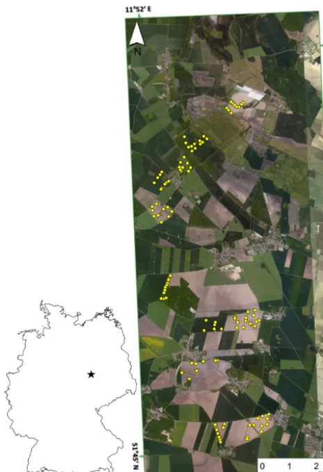
A dominantly agricultural area located near Wulfen, Saxony-Anhalt, Germany, which has been examined by several previ-ous studies (Selige et al., 2006; Brenning et al., 2008; Kühn et al., 2009; Migdall et al., 2009), was selected for this re-search. The mapping area extends from 11.86◦E, 51.74◦N to 11.96◦E, 51.90◦N (Fig. 1), covering a total area of 122 km2. The landscape includes hummocky till plain, outwash plain, loess, and a broad floodplain (Königlich Preußische Geol-ogische Landesanstalt, 1913a, b). The study area is domi-nated by Calcaric Cambisols and Luvic Phaeozems, while the depressional area in the floodplain is primarily Dystric Gleysols (European Commission, 2014). Between 2005 and 2006, 117 locations were sampled from a variety of land-scape positions in 12 different agricultural fields, covering the known feature space for agricultural land in this area. Because all models were calibrated and validated on these samples, evaluation of the resulting maps focused on areas with similar land use (i.e. water bodies and urban areas ex-cluded). Ten of the sample points, also spread across the fea-ture space, were of repeated locations (within 2 m of origi-nal), which helped to insure that random error was reflected in the assessment of estimated error.
Soil horizons identified in the field were sampled at each sampling location. To avoid biases from horizon classifica-tions and to focus on the two major process zones for SOC, the soil profile of 2 m was divided into topsoil and subsoil stocks. The division was defined by the largest decrease in SOC%, as determined by lab analysis, between field identi-fied horizons. Not all profiles were able to be sampled to the full depth of 2 m. In those cases, the properties of the sampled subsoil were assumed to be representative of the remaining depth. Data for the horizons within each stock were com-bined using a thickness-weighted mean, as appropriate. De-scriptive statistics for these observation points are provided in Table 1.
2.2 Modelling
Pre-Figure 1.Locations of sample points and study area within Ger-many.
vious studies have demonstrated the utility of this tool for digital soil mapping (Bui et al., 2006; Minasny and McBrat-ney, 2008; Adhikari et al., 2013; Lacoste et al., 2014). Cu-bist uses a data mining algorithm to build two-tiered models. The top level consists of a series of conditional rules that can utilize both continuous and categorical predictors. For each rule, a MLR equation is produced for predicting the target variable. Cubist’s process for selecting predictors and build-ing the models is described in Quinlan (1993) and Holmes et al. (1999) and will not be repeated here. One advantage of this approach is the interpretability of the produced model, which allows the modeller to assess relationships between the model and physical processes (Bui et al., 2006).
The results of the data mining process are dependent upon the predictors made available to the data mining software. For this reason, we used the large predictor pool method de-scribed by Miller et al. (2015) to identify the optimal mod-els for each of the respective target variables. That method includes a multiple pass test, which reapplies the Cubist al-gorithms to the limited pool selected by the previous run. This helps to insure that the selected predictors have been optimally reduced by the Cubist software, decreasing the
Table 1. Descriptive statistics for the observed target variables. BD: total bulk density (g cm−3); SK: particles>2 mm (%); SOC%:
SOC concentration (%);H: stock thickness (cm); and SOCstock:
mass of organic carbon per unit area of soil (kg m−2).
Topsoil BD SK H SOC% SOCstock
Min. 1.18 0.00 10 0.75 1.80 Median 1.50 1.30 40 1.46 9.27 Mean 1.51 3.15 43.61 1.56 9.82 Max. 1.85 44.70 105 4.03 28.03 SD 0.11 5.50 15.35 0.53 4.49 Subsoil
Min. 1.33 0.00 18 0.02 0.07 Median 1.63 4.07 86 0.23 3.10 Mean 1.63 8.99 86.66 0.26 3.37 Max. 1.96 63.36 155 0.71 9.86 SD 0.13 12.28 32.60 0.13 2.04
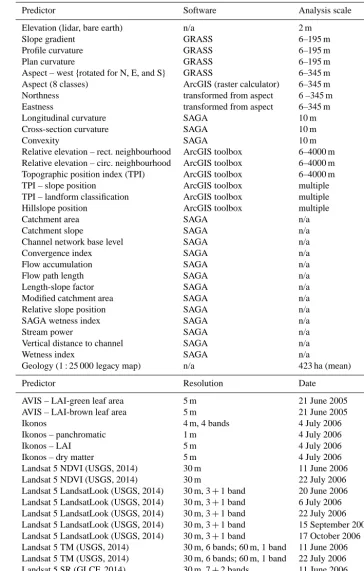
concern of overfitting. The predictor pool for this study in-cluded 410 base maps covering the full extent of the study area (Table 2). These base maps consisted of a legacy ge-ologic map, a variety of remote sensing/spectral products, and digital terrain analysis (DTA). The spectral products ranged from four bands of Ikonos data to a variety of Land-sat data collected at different times in 2006. DTA was con-ducted on a 2 m resolution digital elevation model (DEM), created from lidar data that were also collected in 2006. The DTA base maps included land-surface derivatives based on a wide range of analysis scales (a-scales) and a suite of hydrologic indicators. Land-surface derivatives were cal-culated in GRASS 6.4.3 (Geographic Resources Analysis Support System, http://grass.osgeo.org) and ArcGIS 10.1 (www.esri.com/software/arcgis). Hydrologic indicators were calculated using SAGA 2.1.0 (System for Automated Geo-scientific Analysis, http://www.saga-gis.org/en/index.html).
Table 2.Predictor variables considered in this study.
Predictor Software Analysis scale Elevation (lidar, bare earth) n/a 2 m
Slope gradient GRASS 6–195 m Profile curvature GRASS 6–195 m Plan curvature GRASS 6–195 m Aspect – west{rotated for N, E, and S} GRASS 6–345 m Aspect (8 classes) ArcGIS (raster calculator) 6–345 m Northness transformed from aspect 6 –345 m Eastness transformed from aspect 6–345 m Longitudinal curvature SAGA 10 m Cross-section curvature SAGA 10 m
Convexity SAGA 10 m
Relative elevation – rect. neighbourhood ArcGIS toolbox 6–4000 m Relative elevation – circ. neighbourhood ArcGIS toolbox 6–4000 m Topographic position index (TPI) ArcGIS toolbox 6–4000 m TPI – slope position ArcGIS toolbox multiple TPI – landform classification ArcGIS toolbox multiple Hillslope position ArcGIS toolbox multiple Catchment area SAGA n/a Catchment slope SAGA n/a Channel network base level SAGA n/a Convergence index SAGA n/a Flow accumulation SAGA n/a Flow path length SAGA n/a Length-slope factor SAGA n/a Modified catchment area SAGA n/a Relative slope position SAGA n/a SAGA wetness index SAGA n/a
Stream power SAGA n/a
Vertical distance to channel SAGA n/a
Wetness index SAGA n/a
Geology (1 : 25 000 legacy map) n/a 423 ha (mean) Predictor Resolution Date
Within the extent of the study area, there were a few ar-eas with conditions outside the range observed in the point samples. In these limited cases, extreme predictor values pro-duced model predictions of target variables either far below or above the ranges observed for the respective target vari-ables. To address this issue, spatial predictions were limited to be within 10 % of the observed target variable’s minimum and maximum.
2.3 Propagation of error
For each of the model rules, estimated error was calculated based on the internal fit of the MLR to the data classified within that rule. This estimation provided a measure for the respective uncertainty under each rule. The conditions for the respective rules were used to spatially classify the base maps, thus allowing the estimated errors to be mapped. Measure-ment error, positional error, and limitations of the model to predict the target variable were all empirically encapsulated by the estimated error.
When the target variable was the end product, the uncer-tainty was simply represented by the estimated error. How-ever, when multiple variables were modelled and subse-quently used to calculate the final product, the estimated errors of the component variables propagated through the combination of those variables in the function. In order to map estimated error for the indirect approach of modelling SOCstock, estimated error maps were produced for each of the component variables. These error estimation maps were then combined using standard equations for propagation of error (Mardia et al., 1979; Taylor, 1997; Weisstein, 2014). Although potentially biased by the approximation to a first-order Taylor series expansion, simplified equations for er-ror propagation are more practical and are regularly used in engineering and physical science applications (Goodman, 1960; Ku, 1966). Because covariance between variables has the potential to impact the estimation of SOCstock(Panda et al., 2008; Goidts et al., 2009), we did not assume the vari-ables were independent. The observed residual covariance was thus used to modify the estimated error within the stan-dard equations for propagation of error by multiplication,
σf ≈ |f| r
σA
A
2
+
σB
B
2
+2covAB
AB , (2)
and by addition,
σf ≈ q
σA2+σB2+2covAB, (3)
wheref is the result of the original function (to convert from relative to estimated error), AandB are the real variables, with estimated errorsσAandσB, and their residuals’ covari-ance covAB. In order to calculate a predicted relative error (e.g. σA
A)at unsampled locations, the predicted variable was assumed to accurately represent the variable’s magnitude.
Locations with small ratios between estimated error and predicted values together with large, negative covariances had the potential to produce a calculation taking the square root of a negative. This issue was addressed by not consider-ing the covariance in those limited circumstances. While this solution may have led to an overestimation of error, it pro-vided a means to mathematically calculate estimated error without declaring it to be zero.
3 Results
3.1 Models
3.1.1 Model building and fitting performance
Explicit models were obtained for each of the component variables needed to calculate SOCstockindirectly and for pre-dicting SOCstockdirectly. Models for predicting component variables used a higher quantity of predictors for each of the respective models than the direct modelling approach (Ta-ble 3). With the exception of SOC%, the models for compo-nent variables included a combination of DTA and spectral variables. The SOC% models relied solely on DTA predic-tors for both stocks, but with additional spatial partitioning by geologic map units for the topsoil model. The models for directly predicting the SOCstockused only three DTA predic-tors for the topsoil and only four Landsat predicpredic-tors for the subsoil.
Fitting performances for the component variable models were better than the fitting performances for the direct mod-elling of SOCstock(Table 4). For the component variables,R2 values of subsoil models were only slightly less than the top-soil models. SOC% was the exception by having the lowest fitting performance for the subsoil stock (R2=0.55), while the model for the SOC% topsoil was able to fit observations with anR2of 0.86. However, it was the aim of this research to examine whether the performance of the models was main-tained through the calculation of SOCstock.
Comparison of the SOCstockpredictions by the indirect ap-proach to observed values showed better performance for the topsoil stock (R2=0.73) than for the subsoil stock (R2= 0.34). Fitting performance for directly modelling SOCstock showed the same pattern, but was lower than the indirect ap-proach for both stocks. Analysis of the direct apap-proach’s abil-ity to fit observed values yielded anR2of 0.58 for the topsoil and 0.19 for the subsoil.
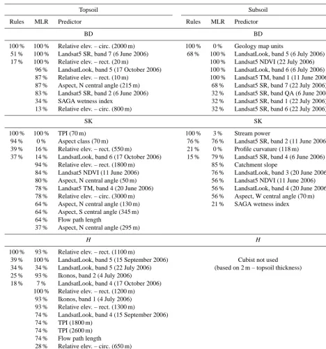
ap-Table 3.Relative use (%) of predictors in models derived by Cubist for the topsoil and subsoil stocks. BD: total bulk density (g cm−3); SK: particles>2 mm (%); SOC%: SOC concentration (%);H: stock thickness (cm); and SOCstock: mass of organic carbon per unit area of soil
(kg m−2).
Topsoil Subsoil
Rules MLR Predictor Rules MLR Predictor
BD BD
100 % 100 % Relative elev. – circ. (2000 m) 100 % 0 % Geology map units
51 % 100 % Landsat5 SR, band 7 (6 June 2006) 68 % 100 % LandsatLook, band 5 (6 July 2006) 17 % 100 % Relative elev. – rect. (20 m) 100 % Landsat5 NDVI (22 July 2006)
96 % LandsatLook, band 5 (17 October 2006) 100 % LandsatLook, band 6 (6 July 2006) 87 % Relative elev. – rect. (10 m) 100 % Landsat5 TM, band 1 (11 June 2006) 87 % Aspect, N central angle (215 m) 68 % Landsat5 SR, band 7 (22 July 2006) 83 % Landsat5 SR, band 2 (6 June 2006) 32 % Landsat5 SR, band QA (6 June 2006) 34 % SAGA wetness index 32 % Landsat5 SR, band 1 (22 July 2006) 13 % Relative elev. – circ. (800 m) 32 % Landsat5 SR, band 6 (22 July 2006)
SK SK
100 % 100 % TPI (70 m) 100 % 3 % Stream power
94 % 0 % Aspect class (70 m) 76 % 76 % Landsat5 SR, band 2 (11 June 2006) 39 % 16 % Relative elev. – rect. (550 m) 21 % 0 % Profile curvature (118 m)
37 % 14 % LandsatLook, band 6 (17 October 2006) 15 % 79 % Landsat5 SR, band 4 (6 June 2006) 94 % Relative elev. – rect. (1800 m) 85 % Catchment slope
84 % Landsat5 NDVI (11 June 2006) 76 % LandsatLook, band 3 (20 June 2006) 80 % Aspect, N central angle (50 m) 56 % Landsat5 NDVI (11 June 2006) 78 % Landsat5 TM, band 4 (20 June 2006) 56 % LandsatLook, band 4 (20 June 2006) 78 % Relative elev. – circ. (3000 m) 56 % Aspect, W central angle (70 m) 64 % Aspect, N central angle (130 m) 21 % SAGA wetness index
64 % Aspect, S central angle (345 m) 64 % Flow path length
37 % Aspect, N central angle (295 m)
H H
100 % 93 % Relative elev. – rect. (1100 m)
39 % 100 % LandsatLook, band 5 (15 September 2006) Cubist not used 34 % 34 % LandsatLook, band 5 (22 July 2006) (based on 2 m – topsoil thickness) 25 % 93 % Ikonos, band 2 (4 July 2006)
18 % 7 % LandsatLook, band 4 (17 October 2006) 100 % Relative elev. – rect. (1200 m)
93 % Ikonos, band 1 (4 July 2006) 93 % Relative elev. – rect. (1300 m)
74 % LandsatLook, band 4 (15 September 2006) 74 % TPI (1800 m)
74 % TPI (2600 m) 74 % Flow path length
28 % Relative elev. – circ. (650 m) 7 % Landsat5 TM, band 6 (11 June 2006)
proach did not improve upon the mean model for predicting the subsoil SOCstock. Although the ME of the direct model for subsoil SOCstockwas also not as good as the other mod-els, it was still an improvement over the mean model.
3.1.2 Model robustness
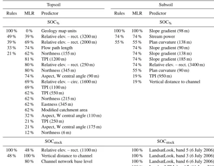
Table 3.Continued.
Topsoil Subsoil
Rules MLR Predictor Rules MLR Predictor
SOC% SOC%
100 % 0 % Geology map units 100 % 100 % Slope gradient (98 m) 49 % 39 % Relative elev. – rect. (3200 m) 74 % 74 % Stream power 39 % 69 % Relative elev. – rect. (2000 m) 55 % 55 % Plan curvature (138 m) 33 % 74 % Flow path length 74 % Slope gradient (90 m) 21 % 62 % Northness (155 m) 74 % Slope gradient (138 m)
81 % TPI (1200 m) 74 % Slope gradient (185 m) 80 % Relative elev. – rect. (250 m) 74 % Relative elev. – rect. (3400 m) 80 % Northness (345 m) 55 % Plan curvature (90 m) 74 % Aspect, W central angle (90 m) 19 % TPI (950 m)
69 % Relative elev. – circ. (1600 m) 19 % Vertical distance to channel 69 % TPI (1100 m)
62 % TPI (550 m) 62 % Northness (215 m) 62 % Eastness (345 m) 62 % Modified catchment area 32 % Aspect, W central angle (110 m) 21 % TPI (250 m)
21 % Aspect, W central angle (175 m) 12 % Northness (6 m)
SOCstock SOCstock
100 % 48 % Relative elev. – rect. (1100 m) 100 % LandsatLook, band 5 (6 July 2006) 48 % 100 % Vertical distance to channel 100 % LandsatLook, band 3 (6 July 2006) 80 % Channel network base level 100 % LandsatLook, band 6 (6 July 2006) 100 % Landsat5 TM, band 7 (11 June 2006)
to maintain more points in the calibration set. However, the model generated for each cross-validation run is different be-cause of differences in calibration sets. The performance of each run is dependent on the randomly selected calibration points’ ability to represent the variation in the remaining val-idation points. For a simple data trend, a single outlier would have minimal effect because only the runs in which it is in-cluded in the validation set – and not used in calibrating the model – would have lower performance values. However, in a complex landscape where similar soil properties can re-sult from different combinations of factors, the concept of an outlier has many more dimensions (Johnson et al., 1990; Phillips, 1998). A point with a similar value can be an out-lier by being a product of a different set of factors. In other words, the problem of induction continues to apply in pre-dictive soil mapping. Further, in the context of error propa-gation, the error estimation from the actual model used seems more appropriate than the mean of error estimations from a series of less robust models.
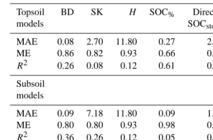
Nonetheless, the models in this study were cross-validated using the k-fold method with 10 iterations. The R2 was naturally reduced in the cross-validation analysis, but the MAE was not as severely affected (Table 5). The R2
val-ues for the respective models all decreased greatly in the cross-validation, except for the topsoil SOC%and the subsoil SOCstockmodels. The subsoil SOCstockmodel already had a lowR2value for the internal fit. In contrast, the MAEs for the cross-validation of the models were not increased enough to present a practical problem. The relative stability of the MAEs also suggests that the estimated uncertainties are also robust. For example, the MAE for both stocks of BD only increased 0.03 g cm−3. Also, the MAE for SOC
Table 4. Fitting performance for the respective models. The model’s efficiency (ME) is the ratio between the model’s mean ab-solute error (MAE) and the MAE that would result from only using the mean value as the model. Cubist reports the ME as relative er-ror, but it is renamed here to avoid confusion with the more common definition of relative error. An ME of greater than 1 indicates that the model is not performing well.
Topsoil BD SK H SOC% Indirect – Direct –
models SOCstock SOCstock
MAE 0.05 1.36 5.90 0.14 1.69 2.27
ME 0.52 0.41 0.47 0.34 0.49 0.66
R2 0.69 0.85 0.71 0.86 0.73 0.58
Subsoil models
MAE 0.06 3.77 5.90 0.06 2.75 1.37
ME 0.58 0.42 0.47 0.59 1.67 0.83
R2 0.67 0.79 0.71 0.55 0.34 0.19
3.1.3 Comparison with previous studies
It is difficult to compare results between SOC mapping stud-ies due to differences in study areas and strategstud-ies for defin-ing SOCstock (i.e. map extent and resolution, sampling den-sity, and consideration of depth). Further, the differences be-tween and variability within methods for estimating compo-nent variables for calculating SOCstockcan have a large im-pact on results, especially bulk density (Liebens and Van-Molle, 2003; Schrumpf et al., 2011) and SOC% (Lowther et al., 1990; Soon and Abboud, 1991; Sutherland, 1998; Bow-man et al., 2002). Also, because model perforBow-mance is de-pendent upon the provided predictors, results of different studies can vary based on the predictors available to and de-rived by the modeller (Miller et al., 2015). However, because the area in this study has been used for several previous stud-ies, some comparisons between methods can be made.
Kühn et al. (2009) examined many of the same samples used in this study and found a coefficient of determination between soil electrical conductivity and soil organic matter to a 1 m depth (kg m−2)ofR2=0.59. Although a slightly dif-ferent calculation, that coefficient of determination is similar to this study’s direct model of topsoil SOCstock(R2=0.58), which used three DTA predictors. However, for the top-soil, the indirect approach in this study produced a SOCstock model with less estimated error and anR2of 0.73. The Kühn et al. (2009) study usually included depths that this study de-fined as subsoil, where the models in this study did not per-form as well (directR2=0.19, indirectR2=0.34).
For the same area as this study, Selige et al. (2006) com-pared MLR and partial least-squares regression for predict-ing SOC% from hyperspectral data with a 6 m spatial res-olution. Although the study by Selige et al. (2006) utilized a higher spectral resolution, the MLR models produced by both that study and the present study had an R2of 0.86 for
Table 5.Cross-validation performance for the respective models. Note that although theR2was severely reduced for most models, the MAE was generally only increased a small amount.
Topsoil BD SK H SOC% Direct –
models SOCstock
MAE 0.08 2.70 11.80 0.27 2.94 ME 0.86 0.82 0.93 0.66 0.85
R2 0.26 0.08 0.12 0.61 0.27 Subsoil
models
MAE 0.09 7.18 11.80 0.09 1.42 ME 0.80 0.80 0.93 0.98 0.86
R2 0.36 0.26 0.12 0.05 0.17
the topsoil SOC%. In the present study, Cubist was able to compensate for the limited spectral information by utilizing several DTA predictors that were available at a high spatial resolution.
3.2 SOCstockmaps
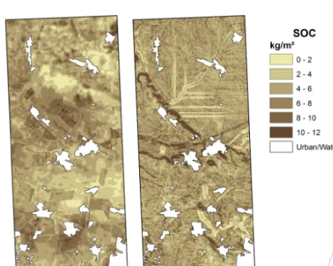
Application of the obtained models and aggregation of the component variable maps by Eq. (1) produced maps of pre-dicted SOCstock for the topsoil and subsoil (Figs. 2 and 3). The respective topsoil and subsoil maps were added together to produce a total SOCstock map to a depth of 2 m (Fig. 4). Although some field boundaries were observed, the domi-nant pattern appeared to be associated with terrain features. This interpretation was supported by the number of DTA pre-dictors selected by Cubist for many of the models. However, it would not have been safe to assume this pattern from the list of selected predictors alone. Certain predictors (i.e. spec-tral data reflecting land use patterns) could have dominated calculations without being the most frequently selected cate-gory of predictors.
The map derived from the direct approach for modelling the topsoil SOCstockemphasizes drainageways. Whereas the map derived by the same approach for the subsoil SOCstock reflects more patterns of land use, especially in the uplands in the southern part of the study area. The topsoil SOCstock map based on the indirect approach has similar overall pat-terns to the direct approach’s map. However, both the topsoil and subsoil maps produced by the indirect approach display greater spatial variation.
thin-Figure 2.Topsoil SOCstockmodelled by (a) the direct approach
and (b) the indirect approach. Overlaid on a hillshade to show rela-tionship with relief and field boundaries.
Figure 3.Subsoil SOCstock modelled by (a) the direct approach and (b) the indirect approach. Overlaid on a hillshade to show rela-tionship with relief and field boundaries.
ner topsoil stocks in these areas and the consistent calculation of a 2 m profile. Consequently, the subsoil is calculated to be thicker in these areas, substantially increasing the subsoil SOCstockprediction compared to other areas of the subsoil.
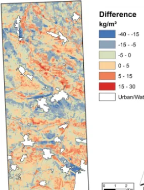
Maps derived by both approaches for the total SOCstock primarily reflected patterns from the topsoil maps because of the higher concentration of SOC that defined the top-soil stock. Nonetheless, modelled storage for the subtop-soil stock contributed about one-third of the prediction of total SOCstockand recognized additional complexity in the SOC landscape. Despite the greater variation in the indirect ap-proach’s prediction of SOCstock, the difference between esti-mates of total SOCstock by the two approaches were within
Figure 4.Total SOCstock(topsoil+subsoil) modelled by (a) the
di-rect approach and (b) the indidi-rect approach. Overlaid on a hillshade to show relationship with relief and field boundaries.
5 kg m−2for the majority of the map area (Fig. 5). Also, the summed SOCstockfor the study area was only 6 % more for the indirect (1.9 Mt) versus the direct (1.8 Mt) approach. The mean SOCstockestimate for the study area by the direct ap-proach was 14.7 kg m−2, whereas the indirect approach esti-mated 15.7 kg m−2.
These aggregated landscape estimates agreed with those made by the Harmonized World Soil Database (HWSD; FAO/IIASA/ISRIC/ISSCAS/JRC, 2012) for this area. The HWSD estimated several soil properties from taxonomic pe-dotransfer functions for static topsoil (0–30 cm) and sub-soil (30–100 cm) depth zones. Within the area of the present study, the HWSD has a cell resolution of approximately 765 m. Calculating SOCstockfrom those data yielded a mean of 8.8 kg m−2. Assuming the characteristics of the subsoil to 100 cm extended to 200 cm, the mean SOCstockwould be 15.3 kg m−2.
3.3 Error estimations
Figure 5. Calculated difference between the direct and indirect approaches of modelling the total SOCstock. Negative values are
where the indirect approach predicted more SOCstockthan the
di-rect approach and positive values are where the indidi-rect approach predicted less.
in stock thickness residuals. The influence of covariance was mostly the same in the subsoil calculations. The exception was a positive covariance between the residuals for mod-elling BD and the percent fine earth. Nonetheless, the co-variances were relatively small with respect to the estimated errors and therefore had a minimal impact on the final calcu-lation of estimated error.
The application of error estimates based on the full range of predicted values in a rule zone to small values in that zone yielded extremely high relative error values. Although the areal extent for this type of situation was very limited, the is-sue needed to be addressed in order to maintain the readabil-ity of the attribute scale. Therefore relative error was capped at one for the original relative error grids, but not thereafter for the calculation of error propagation.
Despite not having as strong of a fitting performance as the indirect approach, the direct approach had lower estimated errors for greater extents of the study area. The mean esti-mated error for the total SOCstockmap derived by the direct approach was 2.81 kg m−2, compared to 8.17 kg m−2for the indirect approach. This behaviour in the models may be ex-plained by the negative covariance between the residuals for many of the variables influencing the SOCstock. The observed covariances did reduce the calculation of error through prop-agation. However, they did not reduce the estimated error for the indirect approach to as low as the estimated error based on the direct modelling approach. It is also useful to note that the residuals for modelling SK and SOC%had a negative and positive skew, respectively, for both stocks (Table 6). Of the residuals for the final prediction of SOCstock, regardless of approach or stock, only the indirect model for the subsoil
Figure 6.Estimated relative error for the total SOCstockmodelled
by (a) the direct approach and (b) the indirect approach.
had strongly skewed residuals. This suggests that error for the indirect model of the subsoil SOCstock may have been overestimated.
The spatial distribution of model rules was an important factor in the resulting maps’ estimated error. The models for the direct approach used fewer rules than the compo-nent variable models, resulting in less spatial variation in the estimated error. However, variation in predicted values did introduce additional spatial variation to the mapping of rel-ative error. Nonetheless, the map of relrel-ative error from the indirect approach was more complex than that resulting from the direct approach. In addition to using more rules for each model, the combined relative estimated error for the indirect approach was further tessellated by the unique intersections of the different spatial distributions of the rules for each com-ponent variable model.
4 Discussion
4.1 Predictor selection
4.1.1 Review of relationships between predictors and environmental conditions
Table 6.Skewness coefficients for the residuals of each model.
BD SK H SOC% Indirect – Direct –
SOCstock SOCstock
Topsoil models −0.25 −1.15 0.17 1.04 0.10 0.37 Subsoil models 0.11 −0.74 −0.17 1.18 −1.61 −0.16
of a single band can be used to distinguish landscape con-ditions. For example, the green band can be used to distin-guish different vegetation from bare soil. However, combi-nations of bands – particularly including the red and NIR bands – have been even more useful for distinguishing the spectral signature of different land uses (Richards, 2006) and the condition of the vegetation (Ashley and Rea, 1975; My-neni et al., 1995; Rasmussen, 1998; Daughtry, 2001; Hatfield et al., 2008). Additional use of TIR emission would resem-ble methods such as the surface temperature/vegetation index for estimating soil moisture (Bartholic et al., 1972; Heilman et al., 1976; Carlson et al., 1994; Li et al., 2009; Petropoulus et al., 2009). Similarly, use of SWIR wavelengths in concert with red and infrared bands would be a way of compensat-ing for the changcompensat-ing effect of soil reflection in dry to wet conditions (Huete, 1988; Lobell and Asner, 2002). Relation-ships between bands in the visible to SWIR range have also been used to predict SOC%and its biochemical composition (Bartholomeus et al., 2008; Gomez et al., 2008; Stevens et al., 2010).
Spectral predictors have been used for both classifica-tion of discrete phenomenon and quantificaclassifica-tion of continu-ous phenomenon on the landscape. Because of the rule-based MLR structure of the Cubist models, spectral predictors used for conditional rules were more likely to be distinguishing discrete features (e.g. vegetation/land use type) than when used within an MLR equation. Continuous features (e.g. veg-etation health) were more likely to be represented in MLR equations.
DTA predictors in this study were all derived from the lidar data for elevation. The land-surface derivatives (e.g. slope gradient, relative elevation) described the surface ge-ometry with which the climate interacts. For example, as-pect has been shown to influence the amount of solar in-solation a hillslope receives (Hunckler and Schaetzl, 1997; Beaudette and O’Geen, 2009). The surface geometry is also known to direct water flow, which affects erosion processes and groundwater recharge (Huggett, 1975; Zevenbergen and Thorne, 1987). Hydrologic predictors (e.g. flow accumula-tion, catchment slope) provided additional information about the relative volume and energy that the water flow may have (Moore et al., 1991; Wilson and Gallant, 2000).
4.1.2 Topsoil model predictors
All of the topsoil models generated by Cubist relied on DTA predictors the most. Of those predictors, different a-scales of
relative elevation, topographic position index (TPI), and as-pect were the most commonly used. With the exception of the direct SOCstockmodel, every topsoil model also included one or two predictors indicative of flow accumulation (i.e. flow path length, SAGA wetness index, or modified catch-ment area).
Aspect at different a-scales influenced predictions for three of the indirect topsoil models. The Cubist-generated model identified decreasing topsoil SOC%on more north fac-ing slopes (155 m a-scale), which corresponds to a poten-tial decrease in plant productivity due to less solar insola-tion. Aspect (215 m a-scale) was also used to predict higher topsoil BD on south- to west-facing slopes, especially on to-pographic (2000 m scale) and micrototo-pographic (20 m a-scale) highs. Additionally, aspect at a variety of a-scales was used to predict decreasing topsoil SK for low-TPI areas fac-ing southeast to southwest. Together, these models suggested a pattern of increased erosion and deposition along the south-ern sides of hillslopes. This type of pattsouth-ern has been observed before in other landscapes and has been attributed to topo-climatic differences such as exposure to storms, differences in temperature regime, rainfall effectiveness, or vegetation density (Kennedy, 1976; Churchill, 1981; Cuff, 1985; van Breda Weaver, 1991).
Although DTA parameters dominated the topsoil models, their predictions were often modified by spectral variables. For example, the primary distinction for predicting topsoil H was between low and high relative elevations. Low rela-tive elevations had a mean topsoilH that was about 20 cm thicker than high relative elevations (1100 m a-scale). Within most MLR equations, however, predictions were increased by less blue and more green reflectance in early July. This combined use of blue and green bands indicated increasing topsoilH with more productive vegetation on wetter soils. In summary, the dominant pattern identified by the model matched the pattern of high and low ground (Bushnell, 1943; Sommer et al., 2008), but the degree of topsoil thinning or thickening was predicted by the vegetation’s response to soil conditions.
DEM based channel network, the model predicted the oppo-site trend of the SOCstockdecreasing with decreasing verti-cal distance to channel. This pattern identified by the model may be explained by a corresponding pattern observed in the model for the topsoilH. In that model, areas low in relative elevation (1100 m a-scale) were predicted to have some of the thickest topsoil stocks. However, within a few of those zones the modelled topsoilHdecreased with decreasing relative el-evation and TPI. This trend in the observed data, as detected by Cubist, was potentially caused by an eroding-out of top-soil sediments closer to the centre of drainageways, in which case, the vertical distance to channel – used in the topsoil SOCstockmodel – may have been more an indicator of prox-imity to the channel than wetness; the threshold was only 0.5 m above the channel modelled from the DEM. Predictors related to surface flow energy would have been expected to be better predictors of this kind of process. However, the up-slope drainage network for much of the map area extended beyond the boundaries of the available data. Thus the use of local elevation data may have been a better proxy in this case compared to the predictors calculated from truncated water-sheds.
4.1.3 Subsoil model predictors
With the exception of SOC%, the subsoil models all used several predictors from Landsat. Selection of Landsat pre-dictors for subsoil models suggested that vegetation charac-teristics or surface soil moisture at different times of the year indicated subsoil conditions. In contrast, the subsoil SOC% model’s complete dependence on DTA predictors suggested that soil property was mostly related to hydrology and that vegetation had little response to or effect on the SOC content in the subsoil.
An example of spectral predictors detecting vegetation characteristics that likely reflected subsoil conditions was the subsoil SK model. All of the MLR equations were strongly influenced by the predictors of stream power, catchment slope, or SAGA wetness index. However, the SK predictions were modified by green reflectance in June and additional Landsat predictors collected at different times of the year that related to the vigour of the vegetation. The weaker or drier the vegetation appeared, the higher the prediction of SK con-tent in the subsoil. Assuming soil moisture conditions did not reach detrimental levels that year, these patterns fit known re-lationships between particle size, soil drainage, and timing to crop maturity (Day and Intalap, 1970; Rawls et al., 1982).
The generated model for subsoil BD most likely utilized a relationship with soil moisture as detected by spectral pre-dictors. In all areas, the MLR equations decreased predic-tions of subsoil BD with increasing reflectance in the blue and SWIR-1 bands along with increasing emission in the TIR band. Increases in the normalized difference vegetation index (NDVI) were used to slightly increase predictions of subsoil BD. The use of the NDVI to offset the decreasing BD
pre-dicted by the other Landsat predictors suggested those vari-ables were indicating soil moisture conditions. Locations that are wetter due to surface runoff would have a greater poten-tial for organic material to be translocated deeper in the soil profile (Schaetzl, 1986, 1990). Also, the association of wetter environments with cooler temperatures and anaerobic condi-tions would also inhibit decomposition (Gates, 1942; Krause et al., 1959; Frazier and Lee, 1971).
The subsoil SOC%model was different than the other sub-soil models generated. Instead of selecting spectral predic-tors, the subsoil SOC% model relied solely on DTA pre-dictors. The model predicted the highest subsoil SOC% on steeper mid-slopes. The pattern of increasing subsoil SOC% from the upper to middle slope fit the landscape translocation model proposed by Sommer et al. (2000). In that study, the SOC% in the Bh horizon increased from the upper slope to the midslope due to lateral translocation. Different than the pattern identified in the present study, the data in Sommer et al. (2000) showed a continued increase in the SOC% of Bh horizons in the downslope position. However, this con-tradiction may be partially explained by aggradation where the slope gradient declines and the topsoil stock has been overthickened by developmental upbuilding (McDonald and Busacca, 1988; Almond and Tonkin, 1999). Also, lateral flow would be expected to return closer to the surface at downs-lope positions. In Sommer et al. (2000), while the upsdowns-lope and midslope profiles had E horizons separating the Bh from A horizons, the downslope Bh horizons were exceptionally thick, with little to no division between them and the A hori-zon. In that situation, the definition of topsoil used in the present study would have grouped the downslope Bh hori-zons into the topsoil stock. Therefore, the Cubist-generated model may have been a simplification of the complex inter-action between topography and lateral flow depth and direc-tion.
The rule groups for subsoil SOC% also differentiated for the plan curvature where the slope gradient was not too high and the stream power index (SPI) was not too low. Concave plan curvatures (138 m a-scale) were predicted to have increasingly higher and convex plan curvatures were predicted to have increasingly lower subsoil SOC%. This relationship with plan curvature matches patterns of water movement identified to be important to soil formation by Huggett (1975), where convergent footslopes have the high-est deposition rates (Pennock and De Jong, 1987). Assum-ing the absence of any restrictive layer below, areas with the highest sediment deposition rates would be expected to also have the highest volume of water infiltration.
these variables, model predictions were dominated by in-creasing reflectance in the red band inin-creasing the estimated subsoil SOCstock. This suggested less productive vegetation corresponding with larger subsoil SOCstock. This trend was counter to the patterns observed in the topsoil models, but was sensible in the context of how the subsoil stock was de-fined for this study. Although the total SOCstockwas less in areas with lower plant productivity, the subsoil SOCstockwas larger relative to other subsoil areas due to the inverse rela-tionship between topsoil and subsoil H used in this study. A thicker topsoil stock would mean a thinner subsoil stock – and vice versa – due to the 2 m depth limit. Regarding the other predictors in this model, increases in SWIR-2 re-flectance could have indicated more plant productivity. How-ever, its use with the TIR band suggested that together they were indicators of wetter soil conditions.
4.2 Unconventional predictor selections
The Cubist software made some intriguing selections in re-gard to predictors that were calculated using alternative ap-proaches. One example of this was the selection of alternative types of aspect predictors. The conversion of aspect to north-ness and eastnorth-ness is generally considered to be the preferred method for addressing the circular problem of using aspect as a predictor. In our approach of including many different predictors in the available pool, we also experimented with simply rotating the central angle (position of 0◦) to each car-dinal direction for creating different aspect predictors. In the models generated for this study, northness and eastness were only selected for the topsoil SOC% model. In contrast, ro-tated versions of aspect were selected for the topsoil SOC%, topsoil BD, and the topsoil and subsoil SK models.
Another example of an intriguing predictor selection by Cubist was the use of bands from the LandsatLook products. These images were limited to four bands (SWIR-1, NIR, red, and TIR) and were smoothed by an algorithm to facilitate im-age selection and visual interpretation. Although the USGS does not recommend the use of these files for data analysis, the Cubist data mining found them to be more useful than the data without LandsatLook processing. Most of these selec-tions can be explained by the greater variety of LandsatLook dates provided in the predictor pool. However, there were a few instances where Cubist chose LandsatLook data over the unprocessed version of the same Landsat data.
4.3 Error propagation
Although both the direct and indirect modelling approaches had base maps with a 2 m resolution available to them, the direct modelling approach produced a more generalized SOCstock map. In terms of predicted error, the cost of try-ing to account for the variation in all of the variables re-lated to the SOCstock appeared to be larger relative errors. The SOCstockmodel from the direct approach, on the other
hand, did not attempt to predict as many variations occur-ring at small phenomenon scales. Because these very local variations were difficult to predict, the estimated error for the direct approach was less than for the indirect approach for most of the map area. Therefore, it may be appropriate to consider the direct modelling approach to be a conservative approach for estimating the SOCstockfor landscapes.
Possible sources of error in the base maps included atmo-spheric conditions for the satellite data and the estimation of bare-earth elevation under dense vegetation for the DEM. Several spectral capture dates were made available in the pre-dictor pool to enable Cubist to not only select the optimal changes in seasonal vegetation characteristics but to also se-lect the image with minimal noise from atmospheric effects such as clouds. Fewer options were available for DTA predic-tors, because all DTA predictors needed to be derived from the same high-resolution DEM. The effect of anomalies in the elevation data was more pronounced for larger a-scales. For example, a small forest plot – located roughly between the two larger cities in the centre of the map area – had not been fully filtered out by the bare-earth algorithm. Any DTA calculation that included this area in its analysis neighbour-hood was incorrectly influenced by those elevation values. The impact on this study’s models was an increased predic-tion of SOCstockin the surrounding area.
The error propagation method used in this study could not directly account for errors in the base maps. Instead, it could only quantify the combined model, base map, and target vari-able error observed at sample locations. Although none of the sample points were in proximity to the before mentioned er-ror in the DEM, this phenomenon of elevation erer-ror affecting scale-dependent predictors would have applied universally, even where the error was less obvious. The higher relative er-ror for both mapping approaches in the area surrounding the known problem in the DEM suggested this potential source of error was at least partially accounted for.
5 Conclusions
This study demonstrated the use of spatial association to pre-dict the SOCstock and the estimated error at unsampled lo-cations within a 122 km2landscape at a high resolution. The Cubist data mining software detected patterns in the observed soil data, which were used to predict soil properties in the greater map region. The ability of the available base maps to predict the variation of those soil properties was quantified for each conditional rule of the respective models. The spa-tial characteristics of the model rules allowed the uncertainty to be mapped along with the target variable prediction.
processes in the soil system. A relationship between selected predictors and known processes provided confidence that their use in the model was not coincidental. The separate modelling of topsoil and subsoil stocks identified a general division between useful predictors for predicting soil prop-erties at different depths. The data mining in this study sug-gested that DTA predictors tend to be most useful for topsoil properties, while spectral characteristics of vegetation and soil moisture tend to be more useful for indicating subsoil properties.
Direct and indirect approaches were tested for predicting the SOCstock with the rule-based, MLR spatial modelling method. Although the spatial patterns in the two maps were generally similar, the indirect approach produced a map with more spatial variation. While attempting to account for more sources of variability resulted in less estimated error for the topsoil (indirect MAE=1.69, direct MAE=2.27), the in-direct approach had a higher potential for error in the sub-soil (indirect MAE=2.75, direct MAE=1.37). Because the direct approach accounts for less variation (topsoil: direct R2=0.58, indirectR2=0.73; subsoil: directR2=0.14, in-directR2=0.34), but also results in a lower total MAE (di-rect MAE=3.64, indirect MAE=4.44), it should be consid-ered a more conservative prediction of the SOCstock’s spatial distribution. The choice of which approach is best will likely depend on a given situation’s need to prioritize the represen-tation of spatial pattern or to minimize estimated error.
Acknowledgements. Data used in this research were collected as part of the Preagro project, funded by the German Federal Ministry of Education and Research (BMBF), under grant reference number 0339740/2. We thank Carsten Hoffmann for his suggestions during the development of this study.
Edited by: B. van Wesemael
References
Adhikari, K., Kheir, R. B., Greve, M. B., and Greve, M. H.: Com-paring kriging and regression approaches for mapping soil clay content in a diverse Danish landscape, Soil Sci., 178, 505–517, doi:10.1097/SS.0000000000000013, 2013.
Almond, P. C. and Tonkin, P. J.: Pedogenesis by upbuilding in an extreme leaching and weathering environment, and slow loess accretion, south Westland, New Zealand, Geoderma, 92, 1–36, doi:10.1016/S0016-7061(99)00016-6, 1999.
Angers, D. A. and Carter, M. R.: Aggregation and organic matter storage in cool, humid agricultural soils, in: Structure and Or-ganic Matter Storage in Agricultural Soils, edited by: Carter, M. R. and Stewart, B. A., CRC Press, Boca Raton, 193–211, 1996. Ashley, M. D. and Rea, J.: Seasonal vegetation differences from
ERTS imagery, Journal of American Society of Photogrammetry, 41, 713–719, 1975.
Bannari, A., Morin, D., Bonn, F., and Huete, A. R.: A review of vegetation indices, Remote Sensing Reviews, 13, 95–120, doi:10.1080/02757259509532298, 1995.
Bartholic, J. F., Namken, L. N., and Wiegand, C. L.: Aerial thermal scanner to determine temperature of soils and of crop canopies differing in water stress, Agronomy J., 64, 603–608, 1972. Bartholomeus, H. M., Schaepman, M. E., Kooistra, L., Stevens, A.,
Hoogmoed, W. B., and Spaargaren, O. S. P.: Spectral reflectance based indices for soil organic carbon quantification, Geoderma, 145, 28–36, doi:10.1016/j.geoderma.2008.01.010, 2008. Batjes, N. H.: Total carbon and nitrogen in the soils of the
world, European J. Soil Sci., 47, 151–163, doi:10.1111/j.1365-2389.1996.tb01386.x, 1996.
Beaudette, D. E. and O’Geen, A. T.: Quantifying the aspect affect: an application of solar radiation modeling for soil survey, Soil Sci. Soc. Am. J., 73, 1345–1352, 2009.
Bowman, R. A., Reeder, J. D., and Wienhold, B. J.: Quantify-ing laboratory and field variability to assess potential for car-bon sequestration, Commun. Soil Sci. Plan., 33, 1629–1642, doi:10.1081/CSS-120004304, 2002.
Brenning, A., Koszinski, S., and Sommer, M.: Geostatistical homogenization of soil conductivity across field boundaries, Geoderma, 143, 254–260, doi:10.1016/j.geoderma.2007.11.007, 2008.
Bui, E. N., Henderson, B. L., and Viergever, K.: Knowl-edge discovery from models of soil properties devel-oped through data mining, Ecol. Model., 191, 431–446, doi:10.1016/j.ecolmodel.2005.05.021, 2006.
Bushnell, T. M.: Some aspects of the soil catena concept, Soil Sci. Soc. Proc., 7, 466–476, 1943.
Cambardella, C. A., Moorman, T. B., Novak, J. M., Parkin, T. B., Karlen, D. L., Turco, R. F., and Konopka, A. E.: Field-scale variability of soil properties in cen-tral Iowa soils, Soil Sci. Soc. Am., 58, 1501–1511, doi:10.2136/sssaj1994.03615995005800050033x, 1994. Carlson, T. N., Gilles, R. R., and Perry, E. M.: A method
to make use of thermal infrared temperature and NDVI measurements to infer surface soil water content and frac-tional vegetation cover, Remote Sensing Reviews, 9, 161–173, doi:10.1080/02757259409532220, 1994.
Churchill, R. R.: Aspect-related differences in badlands slope morphology, Ann. Assoc. Am. Geogr., 71, 374–388, doi:10.1111/j.1467-8306.1981.tb01363.x, 1981.
Cuff, J. R. I.: Quantifying erosion-causing parameters in a New Zealand watershed, in: Soil Conservation, edited by: El-Swaify, S. A., Moldenhauer, W. C., and Lo, A., Soil Conservation Society of America, Ankeny, 99–112, 1985.
Daughtry, C. S. T.: Discriminating crop residues from soil by shortwave infrared reflectance, Agronomy J., 93, 125–131, doi:10.2134/agronj2001.931125x, 2001.
Day, A. D. and Intalap, S.: Some effects of soil mois-ture stress on the growth of wheat (Triticum
aes-tivum L. em Thell), Agronomy J., 62, 27–29,
doi:10.2134/agronj1970.00021962006200010009x, 1970. European Commission: European Soil Database v2, European Soil
Data Centre, available at: http://eusoils.jrc.ec.europa.eu, last ac-cess: 7 October 2014.
Frazier, B. E. and Lee, G. B.: Characteristics and classification of three Wisconsin Histosols, Soil Sci. Soc. Am. J., 35, 776–780, doi:10.2136/sssaj1971.03615995003500050040x, 1971. Gates, F. C.: The bogs of northern lower Michigan, Ecol. Monogr.,
12, 216–254, doi:10.2307/1943542, 1942.
GLCF: Global Land Cover Facility, University of Maryland, avail-able at: http://glcf.umd.edu/data, last access: 19 February 2014. Goidts, E., Van Wesemael, B., and Crucifix, M.: Magnitude and
sources of uncertainties in soil organic carbon (SOC) stock assessments at various scales, Eur. J. Soil Sci., 60, 723–739, doi:10.1111/j.1365-2389.2009.01157.x, 2009.
Gomez, C., Viscarra Rossel, R. A., and McBratney, A. B.: Soil organic carbon prediction by hyperspectral remote sensing and field vis-NIR spectroscopy: An Australian case study, Geoderma, 146, 403–411, doi:10.1016/j.geoderma.2008.06.011, 2008. Goodman, L. A.: On the exact variance of products, J. Am. Stat.
Assoc., 55, 708–713, 1960.
Grace, J.: Understanding and managing the global carbon cycle, J. Ecology, 92, 189–202, doi:10.1111/j.0022-0477.2004.00874.x, 2004.
Grimm, R., Behrens, T., Märker, M., and Elsenbeer, H.: Soil organic carbon concentrations and stocks on Barro Colorado Island – dig-ital soil mapping using random forests analysis, Geoderma, 146, 102–113, doi:10.1016/j.geoderma.2008.05.008, 2008.
Hatfield, J. L., Gitelson, A. A., Schepers, J. S., and Walthall, C. L.: Application of spectral remote sensing for agronomic decisions, Agronomy J., 100, S117–S131, doi:10.2134/agronj2006.0370c, 2008.
Heilman, J. L., Kanemasu, E. T., Rosenberg, N. J., and Blad, B. L.: Thermal scanner measurement of canopy temperatures to es-timate evapotranspiration, Remote Sens. Environ., 5, 137–145, doi:10.1016/0034-4257(76)90044-4, 1976.
Holmes, G., Hall, M., and Frank, E.: Generating rule sets from model trees, Advanced Topics in Artificial Intelligence, Lecture Notes Comput. Sc., 1747, 1–12, doi:10.1007/3-540-46695-9_1, 1999.
Huete, A. R.: A soil-adjusted vegetation index (SAVI), Remote Sens. Environ., 25, 295–309, doi:10.1016/0034-4257(88)90106-X, 1988.
Huggett, R. J.: Soil landscape systems: a model of soil genesis, Geo-derma, 13, 1–22, doi:10.1016/0016-7061(75)90035-X, 1975. Hunckler, R. V. and Schaetzl, R. J.: Spodosol
develop-ment as affected by geomorphic aspect, Baraga County, Michigan, Soil Sci. Soc. Am. J., 61, 1105–1115, doi:10.2136/sssaj1997.03615995006100040017x, 1997. Jobbágy, E. G. and Jackson, R. B.: The vertical
distribu-tion of soil organic carbon and its reladistribu-tion to climate and vegetation, Ecol. Appl., 10, 423–436, doi:10.1890/1051-0761(2000)010[0423:TVDOSO]2.0.CO;2, 2000.
Johnson, D. L., Keller, E. A., and Rockwell, T. K.: Dynamic pedogenesis: new views on some key concepts, and a model for interpreting quaternary soils, Quaternary Res., 33, 306–319, doi:10.1016/0033-5894(90)90058-S, 1990.
Johnston, A. E., Poulton, P. R., and Coleman, K.: Soil organic matter: its importance in sustainable agriculture and carbon dioxide fluxes, Adv. Agronomy, 101, 1–57, doi:10.1016/S0065-2113(08)00801-8, 2009.
Johnston, C. A., Groffman, P., Breshears, D. D., Cardon, Z. G., Cur-rie, W., Emanuel, W., Gaudinski, J., Jackson, R. B., Lajtha, K.,
Nadelhoffer, K., Nelson Jr., D., Mac Post, W., Retallack, G., and Wielopolski, L.: Carbon cycling in soil, Front. Ecol. Environ., 2, 522–528, doi:10.2307/3868382, 2004.
Kay, B. D.: Soil structure and organic carbon: a review, in: Soil Processes and the Carbon Cycle, edited by: Lal, R., Kimble, J. M., Follett, R. F., and Stewart, B. A., CRC Press, Boca Raton, 169–197, 1998.
Kempen, B., Brus, D. J., and Stoorvogel, J. J.: Three-dimensional mapping of soil organic matter content using soil type-specific depth functions, Geoderma, 162, 107–123, doi:10.1016/j.geoderma.2011.01.010, 2011.
Kennedy, B. A.: Valley-side slopes and climate, in: Geomorphol-ogy and Climate, edited by: Derbyshire, E., John Wiley, London, 171–201, 1976.
Khalil, M. I., Kiely, G., O’Brien, P., and Müller, C.: Organic carbon stocks in agricultural soils in Ireland using combined empirical and GIS approaches, Geoderma, 193–195, 222–235, doi:10.1016/j.geoderma.2012.10.005, 2013.
Königlich Preußische Geologische Landesanstalt: Geologische Karte von Preußen und benachbarten Bundesstaten, 1:25,000 (Geological Map of Prussia and adjacent Federal States, 1:25,000), Landesamt f. Geologie und Bergwesen, Halle, Sachsen-Anhalt, Germany, Sheet Wulfen 4137, 1913a.
Königlich Preußische Geologische Landesanstalt: Geologische Karte von Preußen und benachbarten Bundesstaten, 1:25,000 (Geological Map of Prussia and adjacent Federal States, 1:25,000), Landesamt f. Geologie und Bergwesen, Halle, Sachsen-Anhalt, Germany, Sheet Cöthen 4237, 1913b.
Krause, H. H., Rieger, S., and Wilde, S. A.: Soils and forest growth on different aspects in the Tanana watershed of interior Alaska, Ecology, 40, 492–495, doi:10.2307/1929773, 1959.
Kravchenko, A. N., Robertson, G. P., Hao, X., and Bullock, D. G.: Management practice effects on surface total carbon: dif-ferences in spatial variability patterns, Agronomy J., 98, 1559– 1568, doi:10.2134/agronj2006.0066, 2006a.
Kravchenko, A. N., Robertson, G. P., Snap, S. S., and Smucker, A. J. M.: Using information about spatial variability to im-prove estimates of total soil carbon, Agronomy J., 98, 823–829, doi:10.2134/agronj2005.0305, 2006b.
Ku, H. H.: Notes on the use of propagation of error formulas, Jour-nal of Research of the NatioJour-nal Bureau of Standards – C. Engi-neering and Instrumentation, 70C, 263–273, 1966.
Kühn, J., Brenning, A., Wehrhan, M., Koszinski, S., and Som-mer, M.: Interpretation of electrical conductivity patterns by soil properties and geological maps for precision agriculture, Precis. Agric., 10, 490–507, doi:10.1007/s11119-008-9103-z, 2009. Lal, R.: Soil carbon sequestration impacts on global
cli-mate change and food security, Science, 304, 1623–1627, doi:10.1126/science.1097396, 2004.
Lacoste, M., Minasny, B., McBratney, A., Michot, D., Viaud, V., and Walter, C.: High resolution 3D mapping of soil organic car-bon in a heterogeneous agricultural landscape, Geoderma, 213, 296–311, doi:10.1016/j.geoderma.2013.07.002, 2014.
Lemercier, B., Lacoste, M., Loum, M., and Walter, C.: Extrapola-tion at regional scale of local soil knowledge using boosted clas-sification trees: a two-step approach, Geoderma, 171–172, 75– 84, doi:10.1016/j.geoderma.2011.03.010, 2012.
evap-otranspiration estimation from remotely sensed data, Sensors, 9, 3801–3853, doi:10.3390/s90503801, 2009.
Liebens, J. and VanMolle, M.: Influence of estimation proce-dure on soil organic carbon stock assessment in Flanders, Belgium, Soil Use Manage., 19, 364–371, doi:10.1111/j.1475-2743.2003.tb00327.x, 2003.
Lobell, D. B. and Asner, G. P.: Moisture effects on soil reflectance, Soil Sci. Soc. Am. J., 66, 722–727, doi:10.2136/sssaj2002.7220, 2002.
Lowther, J. R., Smethurst, P. J., Carlyle, J. C., and Nam-biar, E. K. S.: Methods for determining organic carbon in podzolic sands, Commun. Soil Sci. Plan., 21, 457–470, doi:10.1080/00103629009368245, 1990.
Lufafa, A., Diédhiou, I., Samba, S. A. N., Séné, M., Khouma, M., Kizito, F., Dick, R. P., Dossa, E., and Noller, J. S.: Carbon stocks and patterns in native shrub commu-nities of Senegal’s Peanut Basin, Geoderma, 146, 75–82, doi:10.1016/j.geoderma.2008.05.024, 2008.
Malone, B. P., McBratney, A. B., and Minasny, B.: Em-pirical estimates of uncertainty for mapping continuous depth functions of soil attributes, Geoderma, 160, 614–626, doi:10.1016/j.geoderma.2010.11.013, 2011.
Mardia, K. V., Kent, J. T., and Bibby, J. M.: Multivariate Analysis, Academic Press, London, United Kingdom, 521 pp., 1979. Martin, M. P., Orton, T. G., Lacarce, E., Meersmans, J.,
Saby, N. P. A., Paroissien, J. B., Jolivet, C., Boulonne, L., and Arrouays, D.: Evaluation of modelling approaches for predicting the spatial distribution of soil organic carbon stocks at the national scale, Geoderma, 223–225, 97–107, doi:10.1016/j.geoderma.2014.01.005, 2014.
Martin, M. P., Wattenbach, M., Smith, P., Meersmans, J., Jolivet, C., Boulonne, L., and Arrouays, D.: Spatial distribution of soil organic carbon stocks in France, Biogeosciences, 8, 1053–1065, doi:10.5194/bg-8-1053-2011, 2011.
McBratney, A. B. and Pringle, M. J.: Estimating average and proportional variograms of soil properties and their poten-tial use in precision agriculture, Precis. Agric., 1, 125–152, doi:10.1023/A:1009995404447, 1999.
McDonald, E. V. and Busacca, A. J.: Record of pre-late Wis-consin giant floods in the Channeled Scabland interpreted from loess deposits, Geology, 16, 728–731, doi:10.1130/0091-7613(1988)016<0728:ROPLWG>2.3.CO;2, 1988.
Meersmans, J., Van Wesemael, B., De Ridder, F., Fallas Dotti, M., De Baets, S., and Van Molle, M.: Changes in organic carbon distribution with depth in agricultural soils in north-ern Belgium, 1960–2006, Global Change Biol., 15, 2739–2750, doi:10.1111/j.1365-2486.2009.01855.x, 2009.
Migdall, S., Bach, H., Bobert, J., Wehrhan, M., and Mauser, W.: Inversion of a canopy reflectance model using hyperspectral im-agery for monitoring wheat growth and estimating yield, Precis. Agric., 10, 508–524, doi:10.1007/s11119-009-9104-6, 2009. Miller, B. A., Koszinski, S., Wehrhan, M., and
Som-mer, M., Impact of multi-scale predictor selection for modeling soil properties, Geoderma, 239–240, 97–106, doi:10.1016/j.geoderma.2014.09.018, 2015.
Minasny, B. and McBratney, A. B.: Regression rules as a tool for predicting soil properties from infrared re-flectance spectroscopy, Chemometr. Intell. Lab., 94, 72–79, doi:10.1016/j.chemolab.2008.06.003, 2008.
Minasny, B., McBratney, A. B., Malone, B. P., and Wheeler, I.: Digital mapping of soil carbon, Adv. Agron., 118, 1–47, doi:10.1016/B978-0-12-405942-9.00001-3, 2013.
Mishra, U., Lal, R., Liu, D., and Van Meirvenne, M.: Pre-dicting the spatial variation of the soil organic carbon pool at a regional scale, Soil Sci. Soc. Am. J., 74, 906–914, doi:10.2136/sssaj2009.0158, 2010.
Moore, I. D., Grayson, R. B., and Ladson, A. R.: Digital terrain modelling: a review of hydrological, geomorpholog-ical, and biological applications, Hydrol. Process., 5, 3–30, doi:10.1002/hyp.3360050103, 1991.
Mulder, V. L., de Bruin, S., Schaepman, M. E., and Mayr, T. R.: The use of remote sensing in soil and terrain mapping – a review, Geoderma, 162, 1–19, doi:10.1016/j.geoderma.2010.12.018, 2011.
Myneni, R. B., Hall, F. G., Sellers, P. J., and Marshak, A. L.: The interpretation of spectral vegetation indexes, IEEE T. Geosci. Re-mote Sens., 33, 481–486, doi:10.1109/36.377948, 1995. Neemann, W.: Bestimmung des Bodenerodierbarkeitsfaktors für
winderosionsgefährdete Böden Norddeutschlands (Determina-tion of soil erodibility factors for wind-erosion endangered soils in Northern Germany), Geologisches Jahrbuch Reihe F, 25, 131 pp., 1991.
Nyssen, J., Temesgen, H., Lemenih, M., Zenebe, A., Haregeweyn, N., and Haile, M.: Spatial and temporal variation of soil organic carbon stocks in a lake retreat area of the Ethiopian Rift Valley, Geoderma, 146, 261–268, doi:10.1016/j.geoderma.2008.06.007, 2008.
Orton, T. G., Pringle, M. J., Page, K. L., Dalal, R. C., and Bishop, T. F. A.: Spatial prediction of soil organic carbon stock using a linear model of coregionalisation, Geoderma, 230–231, 119– 130, doi:10.1016/j.geoderma.2014.04.016, 2014.
Panda, D. K., Singh, R., Kundu, D. K., Chakraborty, H., and Ku-mar, A.: Improved estimation of soil organic carbon storage uncertainty using first-order Taylor series approximation, Soil Sci. Soc. Am. J., 72, 1708–1710, doi:10.2136/sssaj2007.0242N, 2008.
Pennock, D. J. and De Jong, E.: The influence of slope curvature on soil erosion and deposition in hummock terrain, Soil Sci., 144, 209–217, doi:10.1097/00010694-198709000-00007, 1987. Petropoulus, G., Carlson, T. N., Wooster, M. J., and Islam, S.: A
review of Ts/VI remote sensing based methods for the retrieval of land surface energy fluxes and soil surface moisture, Prog. Phys. Geogr., 33, 224–250, doi:10.1177/0309133309338997, 2009. Phachomphon, K., Dlamini, P., and Chaplot, V.: Estimating
car-bon stocks at a regional level using soil information and eas-ily accessible auxiliary variables, Geoderma, 155, 372–380, doi:10.1016/j.geoderma.2009.12.020, 2010.
Phillips, J. D.: On the relations between complex systems and the factorial model of soil formation (with discussion), Geoderma, 86, 1–21, doi:10.1016/S0016-7061(98)00054-8, 1998.
Powlson, D. S., Whitmore, A. P., and Goulding, K. W. T.: Soil carbon sequestration to mitigate climate change: a critical re-examination to identify the true and the false, Eur. J. Soil Sci., 62, 42–55, doi:10.1111/j.1365-2389.2010.01342.x, 2011. Quinlan, J. R.: Learning with continuous classes, Proceedings of the