Do GCMs predict the climate ... or macroweather?

www.earth-syst-dynam.net/4/439/2013/ doi:10.5194/esd-4-439-2013

© Author(s) 2013. CC Attribution 3.0 License.

Earth System

Dynamics

Do GCMs predict the climate . . . or macroweather?

S. Lovejoy1, D. Schertzer2, and D. Varon1

1_{Physics, McGill University, 3600 University St., Montreal, Quebec, Canada}

2_{Université Paris Est, Ecole des Ponts Paris Tech, 6–8, Avenue Blaise Pascal Cité Descartes,}

77455 Marne-La-Vallee Cedex, France

Correspondence to: S. Lovejoy (lovejoy@physics.mcgill.ca)

Received: 16 October 2012 – Published in Earth Syst. Dynam. Discuss.: 22 November 2012 Revised: 9 October 2013 – Accepted: 21 October 2013 – Published: 28 November 2013

Abstract. We are used to the weather–climate dichotomy, yet the great majority of the spectral variance of atmospheric fields is in the continuous “background” and this defines stead a trichotomy with a “macroweather” regime in the in-termediate range from ≈10 days to 10–30 yr (≈100 yr in the preindustrial period). In the weather, macroweather and climate regimes, exponents characterize the type of variabil-ity over the entire regime and it is natural to identify them with qualitatively different synergies of nonlinear dynami-cal mechanisms that repeat sdynami-cale after sdynami-cale. Since climate models are essentially meteorological models (although with extra couplings) it is thus important to determine whether they currently model all three regimes. Using last millen-nium simulations from four GCMs (global circulation mod-els), we show that control runs only reproduce macroweather. When various (reconstructed) climate forcings are included, in the recent (industrial) period they show global fluctua-tions strongly increasing at scales >≈10–30 yr, which is quite close to the observations. However, in the preindus-trial period we find that the multicentennial variabilities are too weak and by analysing the scale dependence of solar and volcanic forcings, we argue that these forcings are unlikely to be sufficiently strong to account for the multicentennial and longer-scale temperature variability. A likely explanation is that the models lack important slow “climate” processes such as land ice or various biogeochemical processes.

1 Introduction

The justification for using GCMs (global circulation mod-els) to model the climate was succinctly expressed by Bryson (1997): “weather forecasting is usually treated as an

initial value problem . . . climatology deals primarily with a boundary condition problem and the patterns and climate de-volving there from.” The main theoretical criticism of this view is that “nonlinear feedbacks (i.e. two way fluxes) be-tween the air, land, and water eliminate an interpretation of the ocean atmosphere and land atmosphere interfaces as boundaries. . . these interfaces become interactive medi-ums. . . (that) must therefore necessarily be considered as part of the predictive system” (Pielke, 1998). In addition, from a modelling perspective, we must consider the problem of coupling of “fast” atmospheric processes with a multitude of “slow” climate processes. Some of these (land use, car-bon cycle, sea ice) are already incorporated into the more ad-vanced GCMs. However other slow processes – such as land ice, deep ocean currents or various biogeochemical processes – are missing and this probably includes some that have yet to be identified. Finally, GCMs which are realistic for one epoch may not be realistic for another. For example, due to the importance of anthropogenic forcings in the recent pe-riod, below we find that the latter become dominant for scales greater than 10–30 yr, whereas in the preindustrial period, the natural forcings and slow processes become dominant only after a somewhat longer period (≈100 yr). In the indus-trial epoch, the GCMs reproduce the (strong) low frequency variability fairly well, whereas in the preindustrial epoch, the (weaker) low frequency variability is poorly reproduced.

100

2

4

10

(

)'$/)

)' -+ _(''

(/,-$)''.

(

('"$() )''+

0 Δ#σ

'"',-

+!'+ "* )''*

12

14

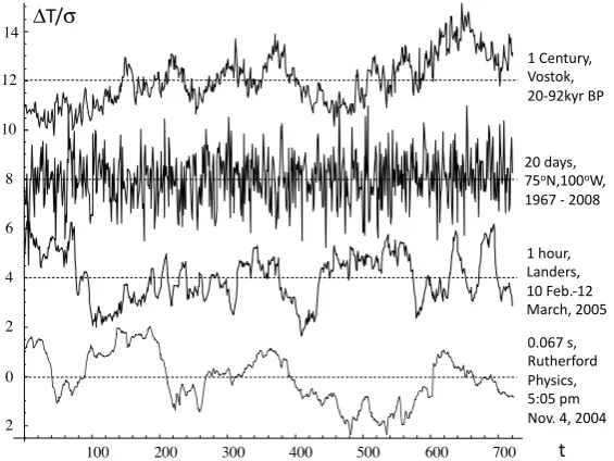
Fig. 1. Dynamics and types of scaling variability: a visual intercomparison displaying representative temperature series from weather, (low frequency) macroweather and climate (H≈0.4, 0.4,−0.4, 0.4, bottom to top, respectively). To make the comparison as fair as possible, in each case, the sample is 720 points long and each series has its mean removed and is normalized by its standard deviation (0.35, 4.49, 2.59, 1.39 K, respectively), the three upper series have been displaced in the vertical by four units for clarity. The resolutions are 0.067 s, 1 h, 20 days and 1 century, respectively, the data are from 4 m above the top of the roof of the Rutherford physics building (Montreal, Quebec), a weather station in Lander, Wyoming, the 20th century reanalysis and the Vostok Antarctic station, respectively. Note the similarity between the type of variability in the weather and climate regimes (reflected in their scaling exponents). This figure is an adaption of a figure in Lovejoy (2013b).

least up to the limits of instrument data i.e.≈150 yr; for a review, see Lovejoy and Schertzer (2013). We see that the weather curves “wander” up or down resembling a drunk-ard’s walk so that temperature differences typically increase over longer and longer periods. In contrast, the 20 day res-olution curve has a totally different character with upward fluctuations typically being followed by nearly cancelling downward ones. Averages over longer and longer times tend to converge, apparently vindicating the conventional idea that “the climate is what you expect”; we anticipate that at decadal or at least centennial scales averages will be virtually constant with only slow, small amplitude variations. How-ever the century-scale curve (top) shows that on the contrary the temperature once again “wanders” in a weather-like man-ner (quantified in Figs. 2 and 3).

There are thus three qualitatively different regimes – not two. While the high frequency regime is clearly the weather and the low frequency regime the climate, the new “in be-tween” regime was described as a “spectral plateau”, then “low frequency weather” and later dubbed “macroweather” since it is a kind of large-scale weather whose statistics are well reproduced by control runs of GCMs (see below); it is not a small-scale climate regime (Lovejoy and Schertzer, 2013). Formally, macroweather may thus be defined as this intermediate regime in which average fluctuations decrease with timescale. The weather–macroweather–climate tri-chotomy has been confirmed in several composite wide-scale

range analyses (Lovejoy and Schertzer, 1986; Pelletier, 1998; Huybers and Curry, 2006b) (see Fig. 2, also Wunsch, 2003) yet the implications have not been widely considered.

If we adopt this trichotomy as an objective basis for cat-egorizing atmospheric dynamics, then a “climate state” is no longer defined by 30 yr averages (a tradition that started in 1935 when the International Meteorological Organization (IMO) adopted the first “climatic normal period” as 1901– 1930). Rather, a climate “state” or “normal” is defined as an average over the entire range of scales out to the scale of minimum temperature variability. As we see in Fig. 3, this is 10–30 yr for the industrial period, but closer to 100 yr for the preindustrial period (c.f. the bottom global scale curves and Fig. 5). The traditional 30 yr IMO definition turns out to be roughly a compromise between the preindustrial and indus-trial timescales. The “climate” is then defined as the variabil-ity of climate states/normals at longer timescales.

The object of this paper is to systematically compare the scale by scale variability of GCM outputs with the corre-sponding variability of various instrumental and proxy data sets in an attempt to answer the question: do GCMs model macroweather, the climate or both? While the analyses of GCMs have not been published elsewhere, several empiri-cal analyses are shown for reference. In the few cases where these are not original to this paper, this is clearly indicated.

Climate Weather

m

Macroweather

Fig. 2. A composite temperature spectrum: the GRIP (Summit) ice coreδ18O, a temperature proxy, low resolution (left, brown) along with the first 91 kyr at high resolution (left, green), with the spectrum of the (mean) 75◦N 20th century reanalysis (20CR, Compo et al., 2011) temperature spectrum, at 6 h resolution, from 1871 to 2008, at 700 mb (right). The overlap (from 10–138 yr scales) is used for calibrating the former (moving them vertically on the log–log plot). All spectra are averaged over logarithmically spaced bins, ten per order of magnitude in frequency. Three regimes are shown corresponding to the weather regime withβw= 2 (the diurnal variation and harmonic at 12 h are visible at the extreme right). The central low frequency weather “plateau” is shown along with the theoretically predictedβmw= 0.2–0.4 regime. Finally, at longer timescales (left), a new scaling climate regime with exponentβc≈1.4 continues to about 100 kyr. Note that a recent revised chronology may modify the very lowest frequencies. Reproduced from Lovejoy and Schertzer (2012b). The black lines are reference lines with the (absolute) slopes indicated.

!%$

$ &

# #

$ #

! !

Δ

'Δ

(

)! )"

paper, in Sect. 3 we compare GCM control (unforced) runs and last millennium (forced) runs and in Sect. 4 we conclude.

2 Methods: fluctuations and their statistics

Let us quantify the analysis of Fig. 1 using fluctuations rather than the spectra shown in Fig. 2. Consider a regime where the mean temperature fluctuation< 1T >varies as a function of timescale (1t) as< 1T >≈1tH, whereH is the fluctua-tion (also called “nonconservafluctua-tion”) exponent (“<.>” indi-cates statistical averaging). WhenH>0 fluctuations increase with scale, whenH <0, they decrease. To see if this explains the “wandering” and “cancelling” in Fig. 1, we must estimate the fluctuations. Although they are usually defined by the ab-solute difference1T betweenT at timetand at timet+1t:

(1T (1t ))diff = |T (t+1t )−T (t )|, (1)

this is only sufficient in the “wandering” regime (more pre-cisely, for 0< H <1). An alternative “tendency fluctuation” is useful in the “cancelling” regime (more precisely, for

−1< H <0) and is obtained by simply removing the overall meanT and calculating the average of the result:

(1T (1t ))trend = 1 1t

t+1t X

t

T0(t )

; T0(t )=T (t )−T . (2)

To cover both regimes (−1< H <1) we should instead use the “Haar fluctuation” which is the absolute difference of the mean betweent andt+1t/2 and betweent+1t/2 and t+1t:

(1T (1t ))Haar = 2 1t

t+1t /2 X

t

T (t )− 2

1t

t+1t X

t+1t /2

T (t )

. (3)

Technically, this corresponds to defining fluctuations us-ing “Haar” wavelets (rather than for example “poor man’s” wavelets which are simply differences (for climate analy-ses with differences see Lovejoy and Schertzer, 1986). The Haar fluctuation is particularly easy to understand since (with proper “calibration”), in regions whereH >0, it can be made very close to the difference fluctuation and in regions where H <0, it can be made close to the “tendency fluctuation”. This means that when the mean Haar fluctuations are plot-ted against scale (1t), that they can be interpreplot-ted either as differences or as averages – depending on whether the fluc-tuations increase or decrease with scale. While other tech-niques such as detrended fluctuation analysis (Peng et al., 1994; Kantelhardt et al., 2002; Monetti et al., 2003) perform just as well for determining exponents, they have the disad-vantage that their fluctuations (which are standard deviations of the residues of polynomial regressions on the running sum of the original series) are not at all easy to interpret (for a summary see Lovejoy and Schertzer, 2012b and for details see Lovejoy and Schertzer, 2012a).

Beyond the first order (mean) statistics, the variation of the fluctuations with scale can be quantified by their q-th order statistics, the structure functionSq(1t )is particularly

convenient:

Sq(1t )= h1t (1t )qi. (4)

Note that Sq is theoretically defined by an ensemble

(sta-tistical) average; in practice we have at most a few realiza-tions – sometimes only a single one – so that the statistics are “noisy”. In practice, Sq is estimated as follows. First,

at any given scale 1t, the Haar fluctuations 1T are esti-mated over all the available disjoint intervals and over all the available realizations. The q-th powers are then aver-aged (the powerq= 2 is the only one discussed in this pa-per, but several values ofq are required for a full multifrac-tal analysis; Schertzer and Lovejoy, 2011). The lags1t are chosen so that there are as close as possible to 20 per or-der of magnitude in scale (since the lags are integer mul-tiples of the smallest resolution, at the smallest 1t, this is at best only approximate). Finally, in order to better match the difference and tendency fluctuations, the Haar fluctu-ations were “calibrated” by multiplying them by a factor of 2 (this worked well for all the series analyzed here). Rel-evant MatLab and Mathematica software are available at http://www.physics.mcgill.ca/~gang/software/index.html.

In a scaling regime, Sq(1t ) is a power law;

Sq(1t )≈1tξ(q), where the exponent ξ(q)=q H−K(q)

and K(q) characterizes the scaling intermittency (with K(1) = 0). In the macroweather regime K(2) is small (≈0.01–0.03), so that the RMS (root mean square) variation S2(1t )1/2 (denoted simplyS(1t )below) has the exponent

ξ(2)/2≈ξ(1) =H. In the climate regime the intermittency correction is a bit larger (Schmitt et al., 1995) (≈0.12) but the error in using this approximation (≈0.06) will be neglected.

3 Review of scaling fluctuation analysis on atmospheric data

Although fluctuation analysis is simple to implement and to interpret, it has not been widely applied to climate data, we now give a brief overview. When S(1t ) is estimated for various in situ, reanalysis, multiproxy and palaeotem-peratures, one obtains Fig. 3 which shows a selection of re-sults from the early reviews (Lovejoy and Schertzer, 2012b, 2013). The key points to note are (a) the three qualita-tively different regimes: weather, macroweather and cli-mate withS(1t )respectively increasing, decreasing and in-creasing again with scale (Hw>0, Hmw<0, Hc>0) and

with transitions at τw≈5–10 days and τc. (b) In the

in-dustrial periodτc≈10–30 yr (1880–present, Fig. 3,

instru-mental curve, see also the new analysis in Fig. 5 discussed below) whereas in the preindustrial period, τc≈50–100 yr

Table 1. Intercomparison of exponents and scales from macroweather (βmw) and climate (βc) exponents and transition scales from var-ious instrumental/palaeocomposite statistical analyses. Theτc values in the top two rows are from data north of 30◦N and are probably anomalously large.

βmw βc Localτc Globalτc

Lovejoy and <1 (central 1.8 ≈400 yr ≈5 yr

Schertzer (1986) England) (poles)

Pelletier (1998) 0.5 (continental 1.7 ≈300 yr –

North America) (Antarctica)

Huybers and 0.56±0.08 1.29±0.13 ≈100 yr –

Curry (2006) (NCEP (several different (tropical sea reanalysis) palaeotemperatures) surface)

Huybers and 0.37±0.05 1.64±0.04 ≈100 yr –

Curry (2006) (NCEP (several different (high latitude reanalysis) palaeotemperatures) continental)

Fig. 5). This comparison indicates that today, anthropogenic warming dominates the global-scale natural variability for scales≈10–30 yr (see Lovejoy, 2013a). (c) The difference between the local- and global-scale fluctuations. (d) The am-plitude of the glacial–interglacial (ice age) transition corre-sponds to overall±2 to±3 K variations, i.e.S(1t )≈4 and 6 K, this “glacial–interglacial window” corresponds to half periods of 30–50 kyr. At least in high latitudes, diverse evi-dence indicates that theS(1t )curve should go through this rectangle.

Note that in scaling regimes, the power spec-trum is E(ω)≈ω−β (ω is the frequency) with β= 1+ξ(2) = 1+2H−K(2) so that ignoring intermit-tency (i.e. K(2)≈0), H >0, H <0 correspond to β >1, β <1 respectively. Hence for macroweather (τc> 1t > τw);

log–log spectra appear as fairly flat “spectral plateaus” (Lovejoy and Schertzer, 1986) (Fig. 2). The present analysis is only of second order (q= 2) statistics, a full analysis would be multifractal (all q). However, the intermittency was found to be small (as characterized by K0(1) which was of the order 0.02) so that this will not much change our conclusions.

The scaling composites mentioned in the introduction agree on the basic scaling picture while proposing some-what different parameter values and transition scalesτc

(Ta-ble 1). Studies of macroweather using other techniques (spec-tra and detrended fluctuation analysis) include those us-ing in situ data (Fraedrich and Blender, 2003; Eichner et al., 2003), sea surface temperatures (Monetti et al., 2003) and ≈1000 yr long Northern Hemisphere reconstructions (Rybski et al., 2006) (see also Lennartz and Bunde, 2009 and Lanfredi et al., 2009). Similarly, Huybers and Curry (2006) used NCEP reanalyses and Blender et al. (2006) (see also Franzke, 2010, 2012, who analysed the Holocene’s

Greenland palaeotemperatures). Finally, multiproxy recon-structions of the Northern Hemisphere (below) yield similar exponents (see Fig. 3 and Lovejoy and Schertzer, 2013).

By considering the fractionally integrated flux models (FIF, i.e. based on cascades, Schertzer and Lovejoy, 1987, 2011; Schertzer et al., 1997) it was argued that whereas in the weather regime, fluctuations depend on interactions in both space and in time, at lower frequencies, only the temporal interactions are important, so thatτw marks a “dimensional

transition”. The basic FIF model predicts macroweather exponents to be typically in the range −0.4< H <−0.2 (i.e. 0.2< β <0.6) and allows the transition scale τw to

be estimated theoretically – and essentially from first prin-ciples – by first considering Earth’s absorbed solar ergy and its average rate of conversion into kinetic en-ergy. This yields an estimate close to the empirical tropo-spheric mean energy flux which is ε≈10−3W kg−1; and which implies a transition scale τw=ε−1/3L2e/3≈10 days

(Le= 20 000 km is the largest distance on Earth; see Lovejoy

and Schertzer, 2010, 2012b). The same transition mecha-nism withεo≈10−8W kg−1yields an ocean weather–ocean

macroweather transition at aboutτw,o≈1 yr (roughly as

ob-served; see Lovejoy and Schertzer, 2012b). Finally, theoret-ical estimates for Mars (taking into account the lower solar irradiance, thinner atmosphere and smaller diameter) yield the predictionsεw,mars≈0.03 W kg−1andτw,mars≈1.5 days.

5444 544

5406

54

Δ

#1*!"2

54

=

Δ

>

12

54 5405

&$ !)"

594405<44

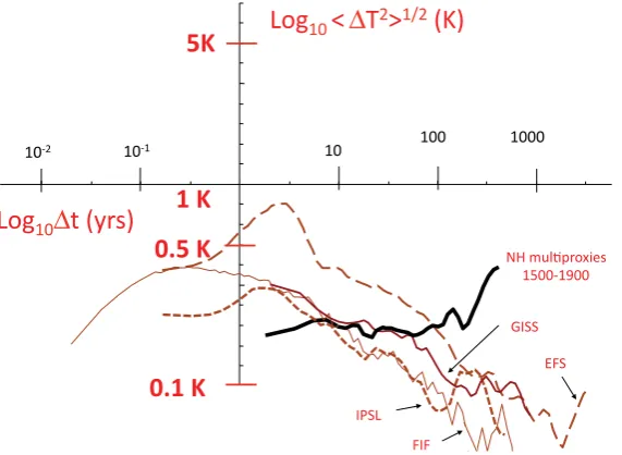
Fig. 4. Control runs versus preindustrial multiproxies: a comparison of the RMS Haar structure functions (S(1t )) for temperatures from the multiproxies Fig. 3 (resolution 1 yr, black, 1500–1900) and GCM control runs (brown dashed, IPSL, EFS monthly), annual resolution GISS-E2-R, (thick brown, continuous) and the FIF stochastic model (thin brown). With the exception of the GISS-E2-R (land, Northern Hemisphere), the data are averaged over the entire globe. The IPSL curve is from a 500 yr control run, the EFS is from a 3000 yr control run; the “bump” at 2–4 yr is a broad quasi periodic model artefact. The reference lines have slopesξ(2)/2 so thatβ= 1+ξ(2) = 0.2, 0.4, 1.8. The amplitude of the Haar structure functions have been calibrated using standard and tendency structure functions and are accurate to within ±25 % (a factor 2 was used).

4 Results

4.1 The unforced low frequency variability of GCMs (control runs)

Since in the stable (H <0) macroweather regime fluctuations converge but in the climate regime they diverge, the aver-ages over the whole regime have the lowest possible vari-ability (S(1t )) and can be used to define “climate states”; the long-term changes in these states (in theH >0 climate regime) correspond to climate changes. From the point of view of GCM modelling, fixed GCM boundary conditions lead to well-defined GCM climates whereas changing bound-ary conditions (climate forcings) lead to climate changes. We therefore expect control runs to yield only macroweather with an exponent characterizing the rate at which the model converges to its climate state. This is confirmed in Fig. 4 where we show S(1t ) from various GCM control runs, i.e. with constant orbital and solar parameters, no volcan-ism, constant greenhouse gases and fixed land use for the IPSL model, the more recent Earth Forecasting System (EFS, Jungclaus et al., 2010) and the GISS-E2-R model (from the CMIP5 data base, curated by G. Schmidt; see also Schmidt et al., 2006 and see Table 3 for model details). We see that their fluctuations are decreasing (i.e. in a macroweather-like man-ner) all the way to their low frequency limits. The challenge for GCMs is therefore to reproduce the growing fluctuations at timescales> τc.

Figure 4 also shows S(1t ) from the low frequency ex-tension of the stochastic FIF cascade model. These struc-ture functions are compared to the corresponding multiproxy functions, we can clearly see a strong divergence between the empirical and FIFS(1t )for1t >≈10–30 yr. With the exception of a spurious “bump” at1t≈2–4 yr scale in the EFS S(1t ), the models do a reasonable job at reproduc-ing the average variability between about one month up to τc≈10–50 yr (depending somewhat on the model and – for

GISS-E2-R – the fact that it is for the Northern Hemisphere, land only with therefore somewhat higher variability). How-ever, beyond that, their mean fluctuations continue to de-cline whereas the empiricalS(1t )starts to rise. The grid-scale analyses of the control runs lead us to exactly the same conclusion; indeed the low frequency exponents are all near the same value corresponding toH≈ −0.4 (β≈0.2; the global-scale exponents are closer toH≈ −0.2,β≈0.6). Fig-ure 4 shows that the GISS-E2-R and IPSL and multiproxy S(Delt at )functions are within≈ ±0.05 K of each other out to 1t≈10 yr while the EFS model has somewhat larger fluctuations. However at longer timescales, the multiproxy S(1t )strongly diverges from the control runs. Whereas the multiproxyS(1t )at 100 yr is≈0.3 K, and rapidly growing, the IPSL, GISS and EFS S(1t )’s are in the range ≈0.1– 0.2 K and are rapidly decreasing.

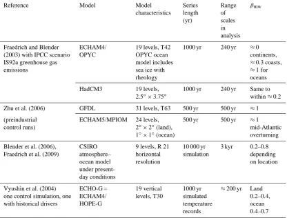
Table 2. Summary of scaling studies of GCM temperatures. All the estimates were made using the DFA method; the spectral exponentβ was determined fromβ= 2α−1, whereαis the conventional DFA exponent (this expression ignores intermittency corrections).

Reference Model Model Series Range βmw

characteristics length of

(yr) scales

in analysis

Fraedrich and Blender ECHAM4/ 19 levels, T42 1000 yr 240 yr ≈0

(2003) with IPCC scenario OPYC OPYC ocean continents,

IS92a greenhouse gas model includes ≈0.3 coasts,

emissions sea ice with ≈1 for

rheology oceans

HadCM3 19 levels, 1000 yr 240 yr Same to

2.5◦×3.75◦ within≈0.2

Zhu et al. (2006) GFDL 31 levels, T63 500 yr 500 yr ≈1

(preindustrial ECHAM5/MPIOM 24 levels, 500 yr 500 yr ≈1

control runs) 2◦×2◦(land), mid-Atlantic

1◦×1◦(ocean) overturning

Blender et al. (2006), CSIRO 9 levels, R 21 10 000 yr 3 kyr 0.2–0.8

Fraedrich et al. (2009) atmosphere– horizontal simulation depending

ocean model resolution on location

under present-day conditions

Vyushin et al. (2004) ECHO-G = 19 vertical 1000 yr ≈200 yr Land

one control simulation, one ECHAM4/ levels, T30 simulated 0.2–0.4,

with historical drivers HOPE-G temperature ocean

records 0.4–0.7

fluctuation analysis technique, although these only consid-ered grid-scale statistics which have a transitionτcat slightly

longer timescales than the global ones in Fig. 3 (see Fig. 8). The basic conclusions of the studies have been pretty uni-form: the low frequency behaviour was scaling, predomi-nantly with 0< β <0.6 (roughly −0.5< H <−0.2, i.e. in the same range as our control runs) and with ocean values a little higher than for land (Table 2). The exponents were robust; for example, with a fixed scenario they were insensi-tive to the use of different models, in the same model, to the addition of greenhouse gases (Fraedrich and Blender, 2003), or in the last 1000 yr in the Northern Hemisphere, to con-stant or to historically changing drivers (Rybski et al., 2008). Finally, models with sophisticated sea ice rheology also had similar scaling (Fraedrich and Blender, 2003). In no cases and at no geographical location was there evidence of an end to the macroweather regime. Apparently, the global-scale IPSL, EFS and GISS-E2-R control run analyses in Fig. 3 are typical.

4.2 The last millennium simulations: the climate or macroweather?

+***

+**

Δ

'!(

0.1 K

1 K

+*

-

0.5 K

+*

1

Δ

,2 +%,'(

&

+.**&+0** ,& # +//*&,**.

$ #

+//*&,**/ +//*&,**/ +//*&,**/

0.2 K

Climate (industrial) macroweather (industrial)

Climate preindustrial) macroweather (preindustrial)

Fig. 5. Recent period instrumental and GCM RMS fluctuations. Comparison of instrumental (CRU, HadCRUT3, black, thick, Northern Hemisphere land only) and GISS-E2-R (dashed: Crowley and Gao volcanic reconstructions (green and blue respectively) and solar only (red); all are for the Northern Hemisphere land only). Gao and Crowley refer to the Gao et al. (2008) and Crowley et al. (2008) volcanic reconstructions discussed in the text. Also shown for reference are the CRU global (orange) and Northern Hemisphere (land and ocean, red) S(1t )for the period 1880–2008. Also shown for reference is the preindustrial multiproxy series (from Fig. 3). Notice that the weather– macroweather transition scale (where the slopes change sign) is roughly 10 yr in the industrial epoch, but closer to 100 yr in the preindustrial epoch (bottom arrows).

differences between the different land use models lead to only small variations, in order to simplify the presentation, we averaged over the three Gao and three Crowley volcanic and the two solar-only runs and compared the results to the Climate Research Unit (CRU) temperature reconstructions (HadCRUT3; Rayner et al., 2006, Fig. 5). It can be seen that over this period, the solar and volcanic forcings only make small differences and that for timescales 1t≈>3 yr, the simulation fluctuation amplitudes all agree quite well with those of the Northern Hemisphere land (however their vari-ability is too weak at shorter times). We conclude that when they are dominated by anthropogenic forcings, the GISS-E2-R simulations have quite accurate variabilities.

We now use the same GISS-E2-R simulations but show the analyses over the preindustrial period, 1000–1900 (Fig. 6). We see that the behaviour is radically different. First, the simulations with the solar forcings only are very close to the control run (indicating that their forcings are quite weak). In contrast, the volcanically forced runs show that the am-plitudes are too strong at scales1t≈<100 yr, but quickly decrease and become too weak for longer1t. Interestingly, at1t≈τc(≈20 yr) the sign of the volcanic slopes changes.

However, the series with volcanic forcings vary in the oppo-site direction from the data: first constant or growing and then decreasing with scale. When compared with the multiproxies we see that whereas at1t≈10 yr, the volcanic forcings are factors 2–4 too large, at 400 yr scales they are factors 1.5– 4 too small. In contrast, the series with solar only forcing

are too weak by a roughly constant factor≈1.5 and≈4 at 10 yr and≈400 yr, respectively. It is interesting to note that theseS(1t )are quite close (generally within a factor of 2) to those obtained on outputs of the simplified Zebiak–Cane model published in Mann et al. (2005) (work in progress with C. Varotsos). In conclusion, the GISS-E2-R results are differ-ent for the differdiffer-ent epochs although only the results of the recent period seem fully realistic.

Focusing on the preindustrial period (here 1500–1900), we considered two other GCMs and their last millennium simulations: the ECHO-G “Erik the Red” simulation (von Storch et al., 2004) and two EFS simulations (Jungclaus et al., 2010). The ECHO-G simulation was chosen because in the IPCC AR4 (Solomon et al., 2007) twelve different mil-lennium simulations were compared (although only two were full GCMs) and it was noted that ECHO-G had significantly stronger low frequency variability than any of the others. In-deed, Osborn et al. (2006) found that, due to initialization problems and lack of sulfates, ECHO-G was only reliable over the period 1300–1900 AD; our range 1500–1900 AD was free of these problems.

5444

544

54

Δ

#1*!"2

0.1 K

1 K

54

0.5 K

54

=

Δ

6

>

5/6

12

#!

'

! *

!(* '

&$0 !)" 594405<44

Fig. 6. Preindustrial multiproxy and GISS-E2-R RMS fluctuations. Same as Fig. 5 except for the preindustrial period (1000–1900), the lower black curve is the GISS-E2-R control run from Fig. 4.

0.25 % are considered respectively low and high solar forc-ing values (see Krivova and Solanki, 2008) for a recent re-view. In these terms, the ECHO-G forcings were “high” (0.25 %) whereas the EFS simulations were run at both 0.1 and 0.25 % levels. The GISS-E2-R simulations compared both Steinhilber et al. (2009) and Vieira et al. (2011) solar reconstructions corresponding to smaller (0.06 and 0.10 %) variations. Only the pre-1610 part of the reconstructions were based on the 10Be-based reconstructions so that over the range 1500–1900 AD these percentages capture the main so-lar reconstruction differences (see below and Table 4 for a summary and Fig. 9 for an analysis of some of the forcings). We have already discussed the GISS-E2-R analyses; for the preindustrial ECHO-G, EFS analyses (Figs. 7 and 8: global- and grid-scales respectively) the key conclusions are the following.

a. The overall EFS variability is very close to the corre-sponding control run (Fig. 4); it is much too weak. b. The global-scale low frequency variability (Fig. 7) of

the GCM’s decrease with increasing1t and the EFS macroweather behaviour hasS(1t )≈1t−0.4. c. The grid-scale ECHO-G simulation (but not EFS,

Fig. 8) has relatively realistic multicentennial variabil-ity (close to the multiproxies) with roughly the same τcandH as the data and the multiproxies.

These results are quite similar to those obtained from the analysis of the GISS-E2-R simulations discussed earlier. Similarly, Franzke et al. (2013) used spectral analysis and concluded that the ratios of low and high frequency variabil-ity of GCMs and palaeodata were significantly different, but

they did not specifically consider the macroweather–climate transition, nor did they clearly attribute the problem to a lack of centennial and lower frequency GCM variability.

4.3 Discussion

We reviewed evidence that the variability of the atmo-sphere out toτc≈10–30 yr (recent period) andτc≈100 yr

(preindustrial) is dominated by weather and macroweather dynamics. τc marks a qualitative transition between a

higher frequency regime whose fluctuations decrease with scale (H <0), and the climate regime where they in-crease with scale (H >0). We showed that control runs of GCMs (studied in the literature and confirmed here) dis-play macroweather regimes converging in power law man-ner to their “climates” with no low frequencyH >0 regime right out to their low frequency limits: as expected, their low frequency variability is too weak. In comparison, start-ing from scalesτc≈10–30 yr, forced runs during the recent

(1880–present) period showed fluctuations in globally aver-aged temperatures strongly increasing and were quite realis-tic, i.e. close to the recent period’s instrumental global vari-abilities. Focusing on the preindustrial period – where the multiproxies showed that temperature fluctuations increase afterτc≈50–100 yr – we found (with the partial exception

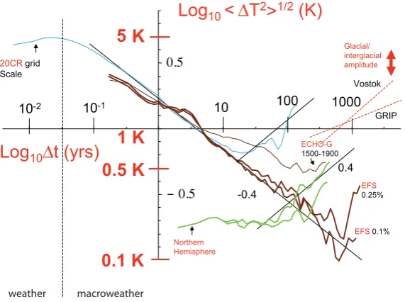
Fig. 7. Pre-1900 forced runs versus data, global scale: this is the same as Fig. 4 (global averages) except that the pre-1900 forced ECHO-G (thin brown) and EFS models (thick brown) are analysed. The upper right dashed lines indicate the rough ranges of the Vostok and GRIP (Greenland ice core) fluctuations at multicentennial scales, and the arrow the glacial–interglacial variations at 50–100 kyr. Also shown are the global- and grid-scaleS(1t )from the 20th century reanalysis (blue) as well as two curves for the multiproxies (green) shown in Fig. 3 (the top corresponds to the period 1500–1980, the bottom to the period 1500–1900).

macroweather weather

Fig. 8. Grid-scale, forced pre-20th C RMS fluctuations: the same as Fig. 7 except for grid-scale analyses (the green Northern Hemisphere multiproxy curves were added for reference, see Fig. 4). Again, the EFS model has low frequencies that are too weak, but even ECHO-G has weak variability and the low frequency tendency is not clear (i.e. is it starting to rise at1t≈500 yr?).

Although it seems plausible that if the climate forcing was of the right type and was sufficiently strong aH >0 climate regime would appear, it is not trivial to find the appropi-ate forcings. This is because in a recent paper (Lovejoy and Schertzer, 2012c), we examined the scale dependence of fluc-tuations on the radiative forcings (1RF) of several solar and

volcanic reconstructions, finding that they generally were scaling with1RF≈A 1tHR(see Table 4 and Fig. 9 discussed

below). Only if HR≈HT≈0.4, would scale independent

amplification–feedback mechanisms suffice. For volcanic re-constructions we foundHR,vol≈ −0.3, which quantifies the

Solar

Volcanic

10

10

Log

t (yrs)

Log

10

<

Δ

(

RF)

2>

1/2

(K)

2Wm-2

0.1 Wm-2

1 Wm-2

1yr

0.01 Wm-2

Gao 2009

Krivova 2007

Wang 2005 (background) Crowley

2000

10

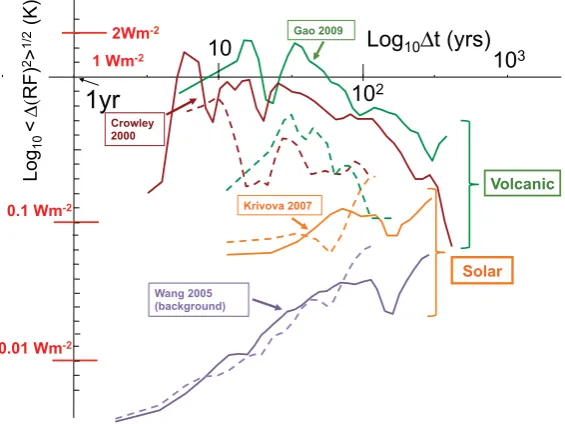
Fig. 9. Radiative forcings from various solar and volcanic reconstructions: a comparison of RMS Haar fluctuations for two solar and two volcanic radiative forcing reconstructions (RF; units Wm−2). The dashed lines are for the period 1900–present, the solid lines for the period 1500–1900 (volcanic), 1610–1900 (solar). Note that the Wang et al. (2005) curve is only for the background solar forcing (without the 11 yr cycle) whereas the Krivova et al. (2007) curve has a 10 yr resolution. The volcanic series were from reconstructions of stratospheric sulfates using ice core proxies. All the structure functions have been increased by a factor of 2 so that they are roughly “calibrated” with the difference (H >0) and tendency (H <0) fluctuations; see Table 4. The basic forcings have roughly the same scaling properties in the industrial and preindustrial period, only the amplitudes of the volcanic forcings are slightly weaker in the recent epoch.

is unlikely that they can be explained by forcings which de-crease with scale. Considering the sunspot-based solar re-constructions, we foundHR,sol≈ +0.4 hence they grow with

scale but, in contrast, the10Be reconstructions (used for the pre-1610 part of the forcing in the GISS-E2-R simulations) hadHR,sol≈ −0.4 (decreasing; they cannot both be

realis-tic). While the sunspot-based reconstructions have roughly HR,sol≈HTso that they potentially have scale-independent

climate sensitivities, if solar forcing was the dominant mech-anism for driving the climate at centennial and millennial scales, the amplification/feedback factors would have to be very large: Lovejoy and Schertzer (2012c) estimate that fac-tors≈15–20 would be necessary.

Table 4 gives the parameters estimated in Lovejoy and Schertzer (2012c) derived over the entire length of the forc-ing reconstructions up to the present. However, in Fig. 5 we saw that the decadal- and centennial-scale temperature vari-ability (S(1t ))was quite different in the industrial and prein-dustrial periods. If the inprein-dustrial solar and/or volcanic forc-ings were much stronger, then they could potentially explain the anomalously high industrial temperature variability, it is therefore interesting to compare the forcings in the different periods. Figure 9 shows the result for the volcanic forcings (the Gao and Crowley reconstruction discussed earlier, back to 1500) as well as two solar sunspot-based reconstructions (back to 1610 only). Notice that the overall form of the forc-ings (roughly scaling, linear on log–log plots) is the same

for the industrial and preindustrial periods although their amplitudes have changed: the industrial period has slightly weaker (not stronger) volcanic forcings, and roughly un-changed solar forcings. These forcings therefore cannot ex-plain the much larger amplitude (decadal and longer period) industrial-epoch temperature variabilities, the latter are pre-sumably due to the increases in greenhouse gases.

5 Conclusions

Table 3. Details of the climate simulations.

Model system Model components GCM Experiment Series

and references characteristics length

(yr)

ECHO-G ECHAM4 (Roeckner et al., 19 vertical “Erik the 1000

(von Storch et al., 1996), HOPE-G (Wolff et al., levels, T30, Red”, 1000 AD to

2004) 1997) (3.75◦ present,

resolution) ≈0.25 % solar forcing

Earth Forecasting System ECHAM5 GCM MPIOM ocean 19 levels, Millennium, 1000 with

(EFS) model (Jungclaus et al., 2006), T31 (3.75◦ solar forcing full

(Jungclaus et al., carbon cycle module HAMOCC5 resolution) 0.1, 0.25 %, forcing,

2010) (Wetzel et al., 2006), land surface 1000 AD to 3000 yr

scheme JSBACH (Raddatz et al., present control

2007) run

IPSL climate system model: LMDZ GCM (Hourdin et al., 19 levels, Control run: 500 yr

IPSL-CM4 2006), ORCA2 Ocean model, 2.5◦×3.75◦ 1910–2410,

(Madec et al., 1998), LIM grid for IPCC

Sea ice model (Fichefet and AR4

Morales Maqueda, 1997), ORCHIDEE land surface model (Krinner et al., 2005)

GISS-E2-R Includes ocean, tracer and sea ice 20 levels, 8 runs 1150 yr

models, incorporates land use 2◦×2.5◦ varying (850–2000 AD) changes, from the CMIP5 data grid forcings,

base, curated by G. Schmidt, see land use also Schmidt et al. (2006,

2011, 2012)

In both epochs the global surface temperature has a min-imum RMS fluctuation of about ±0.1 K (Figs. 3, 5) after which it increases in roughly a scaling manner until attain-ing from ±2 to ±3 K at time periods corresponding to the glacial–interglacial transition (periods of about ≈100 kyr, see Fig. 3). While the lower frequency regime was identi-fied with the climate, the middle intermediate regime which was dominated by (coupled ocean–atmosphere) weather pro-cesses was termed “macroweather”. The challenge of GCMs is therefore to reproduce the slow processes that become dominant at scales between decades and centuries and that remain dominant up to tens of millennia. With the help of the GISS E2-R, we confirmed that the difference between the in-dustrial and preinin-dustrial epochs is a consequence of the fact that in the industrial period the natural forcings (essentially solar and volcanic) are dominated by anthropogenic effects.

The picture that emerges from our analyses of tempera-tures, reconstructed forcings and model outputs is that of fast weather–ocean processes becoming successively weaker at longer and longer timescales being eventually dominated by new climate processes that become stronger and stronger. These processes presumably include both the responses to external climate forcings (often nonlinearly amplified) as well as low frequency variability generated by new slow

climate processes. Elsewhere (Lovejoy and Schertzer, 2012b, c) with the help of palaeotemperature analyses (e.g. Fig. 3), we argued these new responses and processes are apparently dominant from the end of the macroweather regime until scales of ten or more millennia, beyond which orbital forc-ings are important.

Table 4. A comparison of various climate radiative forcings (RF) discussed in Lovejoy and Schertzer (2012c), estimated over the length of time indicated in the fourth column up to the present (Fig. 9 shows industrial and preindustrial analyses for selected series). The exponents were estimated to the nearest 0.1 and the prefactorsAare for the formulah(1RF)2i1/2=A 1tξ(2)/2with1texpressed in years.

Series Physical Reference Series Series Scale Prefactor ξ(2)/2

type basis length resolution range A ≈H_R∗

(yr) (yr) analysed (W m−2)

(yr)

Solar

Sunspot-based Lean

≈400

1 10–400 0.035 0.4

(2000)

Solar

Wang et 1 10–400 0.0074 0.4

al. (2005)

Krivova et 10 20–400 0.015 0.4

al. (2007)

TIMS 8.7 6 h 1–8 0.04 0.4

satellite

10_Be

Steinhilber 9300 5 yr 80–9300 0.4 −0.3

et al. smoothed to

(2009) 40 yr

Shapiro et 9000 1 yr 40–9000 3.5 −0.3

al. (2011) smoothed to

20 yr

Volcanic

Volcanic Crowley 1000 1 yr 60–1000 2.0 −0.3

indices, (2000) smoothed to

ice cores, 30 yr

radiance models

Ice core Gao et al. 1500 1 yr 60–1000 2.5 −0.3

sulfates (2008) smoothed

radiance 30 yr

models

∗_{The solar series all have low intermittencies so thatξ(2)/2≈Hwhereas the Crowley and Goa et al. volcanic series have high}

intermittencies so thatH≈ξ(2)/2+C1≈ −0.2, whereC1≈0.16 is the intermittency correction.

reconstructions in Lovejoy and Schertzer (2012c) found that these typically become weaker – not stronger – with scale and are unlikely to be strong enough to provide sufficient forcing at multicentennial scales and beyond (see Fig. 9). Therefore, even if the reconstructed solar and volcanic forc-ings turn out to be unrealistically weak and the true forcing levels are substantially higher, as long as this qualitative (decreasing) character continues to hold, they will still not be able to fully explain the low frequency climate variability. Barring the discovery of a new source of low frequency external forcing, it is hard to escape the conclusion that one must introduce new slow mechanisms of internal climate variability (these might include new internal couplings with existing solar and volcanic forcings). Such new mechanisms must have broad spectra; this suggests that their dynamics involve nonlinearly interacting spatial degrees of freedom. Promising candidates include deep ocean currents, land ice and various biogeochemical processes.

Acknowledgements. We thank G. Schmidt and R. Pielke Sr. for helpful discussions and comments. The public discussion version of the paper also contained useful comments. Anonymous referees of Nature Climate change as well as a GRL editor are thanked for comments on earlier, shorter versions. This work was unfunded; there are no conflicts of interest.

Edited by: A. Kleidon

References

Blender, R., Fraedrich, K., and Hunt, B.: Millennial climate vari-ability: GCM-simulation and Greenland ice cores, Geophys. Res. Lett., 33, L04710, doi:10.1029/2005GL024919, 2006.

Compo, G. P., Whitaker, J. S., Sardeshmukh, P. D., Matsui, N., Al-lan, R. J., Yin, X., Gleason, B. E., Vose, R. S., Rutledge, G., Bessemoulin, P., Brönnimann, S., Brunet, M., Crouthamel, R. I., Grant, A. N., Groisman, P. Y., Jones, P. D., Kruger, A. C., Kruk, M., Marshall, G. J., Maugeri, M., Mok, H. Y., Nordli, Ø., Ross, T. F., Trigo, R. M., Wang, X. L., Woodruff, S. D., and Worley, S. J.: The Twentieth Century Reanalysis Project, Q. J. Roy. Meteorol. Soc., 137, 1–28, doi:10.1002/qj.776, 2011.

Crowley, T. J.: Causes of Climate Change Over the Past 1000 Years, Science, 289, 270–273, doi:10.1126/science.289.5477.270, 2000.

Crowley, T. J., Zielinski, G., Vinther, B., Udisti, R., Kreutzs, K., Cole-Dai, J., and Castellano, E.: Volcanism and the Little Ice Age, PAGES Newslett., 16, 22–23, 2008.

Eichner, J. F., Koscielny-Bunde, E., Bunde, A., Havlin, S., and Schellnhuber, H.-J.: Power-law persistance and trends in the at-mosphere: A detailed studey of long temperature records, Phys. Rev. E, 68, 046133-40, doi:10.1103/PhysRevE.68.046133, 2003. Fichefet, T. and Morales Maqueda, M. A.: Sensitivity of a global sea ice model to the treatment of ice thermodynamics and dynamics, J. Geophys. Res., 102, 12609–12646, 1997.

Fraedrich, K. and Blender, K.: Scaling of Atmosphere and Ocean Temperature Correlations in Observations and Climate Models, Phys. Rev. Lett., 90, 108501–108504, 2003.

Fraedrich, K., Blender, R., and Zhu, X.: Continuum Climate Vari-ability: Long-Term Memory, Scaling, and 1/f-Noise, Int. J. Mod-ern Phys. B, 23, 5403–5416, 2009.

Franzke, C.: Long-range dependence and climate noise characteris-tics of Antarctica temperature data, J. Climate, 23, 6074–6081, doi:10.1175/2010JCL13654.1, 2010.

Franzke, C.: Nonlinear trends, long-range dependence and cli-mate noise properties of temperature, J. Clicli-mate, 25, 4172–4183, doi:10.1175/JCLI-D-11-00293.1, 2012.

Franzke, J., Esper, J., and Brönnimann, S.: Spectral biases in tree-ring climate proxies, Nat. Clim. Change, 3, 360–364, doi:10.1038/Nclimate1816, 2013.

Gao, C. G., Robock, A., and Ammann, C.: Volcanic forcing of climate over the past 1500 years: and improved ice core-based index for climate models, J. Geophys. Res., 113, D23111, doi:10.1029/2008JD010239, 2008.

Hourdin, F., Musat, I., Bony, S., Braconnot, P., Codron, F., Dufresne, J.-L., Fairhead, L., Filiberti, M.-A., Friedlingstein, P., Grandpeix, J.-Y., Krinner, G., LeVan, P., Li, Z.-X., and Lott, F.: The LMDZ4 general circulation model: climate performance and sensitivity to parametrized physics with emphasis on tropical convection, Clim. Dynam., 27, 787–813, doi:10.1007/s00382-006-0158-0, 2006.

Huang, S. P., Pollack, H. N., and Shen, P.-Y.: Temperature trends over the past five centuries reconstructed from borehole temper-atures, Nature, 403, 756–758, 2000.

Huybers, P. and Curry, W.: Links between annual, Milankovitch and continuum temperature variability, Nature, 441, 329–332, doi:10.1038/nature04745, 2006.

Jungclaus, J. H., Keenlyside, N., Botzet, M., Haak, H., Luo, J.-J., Latif, M., Marotzke, J.-J., Mikolajewicz, U., and Roeckner, E.: Ocean Circulation and tropical variability in the coupled model ECHAM5/MPIOM, J. Climate, 19, 3952–3972, 2006.

Jungclaus, J. H., Lorenz, S. J., Timmreck, C., Reick, C. H., Brovkin, V., Six, K., Segschneider, J., Giorgetta, M. A., Crowley, T. J., Pongratz, J., Krivova, N. A., Vieira, L. E., Solanki, S. K., Klocke, D., Botzet, M., Esch, M., Gayler, V., Haak, H., Raddatz, T. J., Roeckner, E., Schnur, R., Widmann, H., Claussen, M., Stevens, B., and Marotzke, J.: Climate and carbon-cycle variability over the last millennium, Clim. Past, 6, 723–737, doi:10.5194/cp-6-723-2010, 2010.

Kantelhardt, J. W., Zscchegner, S. A., Koscielny-Bunde, K., Havlin, S., Bunde, A., and Stanley, H. E.: Multifractal detrended fluctu-ation analysis of nonstfluctu-ationary time series, Physica A, 316, 87– 114, 2002.

Krinner, G., Viovy, N., De Noblet-Ducoudre, N., Ogeé, J., Polcher, J., Friedlingstein, P., Ciais, P., Sitch, S., and Prentice, I. C.: A dynamic global vegetation model for studies of the cou-pled atmosphere-biosphere system, Global Biogeochem. Cy., 19, Gb1015, doi:10.1029/2003gb002199, 2005.

Krivova, N. A. and Solanki, S. K.: Models of Solar Irradiance Vari-ations: Current Status, J. Astrophys. Aston., 29, 151–158, 2008. Krivova, N. A., Balmaceda, L., and Solanski, S. K.: Reconstruction of solar total irradiance since 1700 from the surface magnetic field flux, Astron. Astrophys., 467, 335–346, doi:10.1051/0004-6361:20066725, 2007.

Lanfredi, M., Simoniello, T., Cuomo, V., and Macchiato, M.: Dis-criminating low frequency components from long range persis-tent fluctuations in daily atmospheric temperature variability, At-mos. Chem. Phys., 9, 4537–4544, doi:10.5194/acp-9-4537-2009, 2009.

Lean, J. L.: Evolution of the Sun’s Spectral Irradiance Since the Maunder Minimum, Geophys. Res. Lett., 27, 2425–2428, 2000. Lennartz, S. and Bunde, A.: Trend evaluation in records with long

term memory: Application to global warming, Geophys. Res. Lett., 36, L16706, doi:10.1029/2009GL039516, 2009.

Ljundqvist, F. C.: A new reconstruction of temperature variability in the extra – tropical Northern Hemisphere during the last two millennia, Geograf. Ann. A, 92, 339–351 doi:10.1111/j.1468-0459.2010.00399.x, 2010.

Lovejoy, S.: Scaling fluctuation analysis and statistical hypothe-sis testing of anthropogenic warming, Clim. Dynam., submitted, 2013a.

Lovejoy, S.: What is climate?, EOS, 94, 1–2, 2013b.

Lovejoy, S. and Schertzer, D.: Scale invariance in climatological temperatures and the spectral plateau, Ann. Geophys., 4B, 401– 410, 1986.

Lovejoy, S. and Schertzer, D.: Towards a new synthesis for atmo-spheric dynamics: space-time cascades, Atmos. Res., 96, 1–52. doi:10.1016/j.atmosres.2010.01.004, 2010.

Lovejoy, S. and Schertzer, D.: Haar wavelets, fluctuations and struc-ture functions: convenient choices for geophysics, Nonlin. Pro-cesses Geophys., 19, 513–527, doi:10.5194/npg-19-513-2012, 2012a.

Lovejoy, S. and Schertzer, D.: Low frequency weather and the emer-gence of the Climate, in: Extreme Events and Natural Hazards: The Complexity Perspective, edited by: Sharma, A. S., Bunde, A., Baker, D., and Dimri, V. P., AGU monographs, Washington, D.C., 231–254, 2012b.

Lovejoy, S. and Schertzer, D.: The Weather and Climate: Emergent Laws and Multifractal Cascades, Cambridge University Press, Cambridge, 496 pp., 2013.

Madec, G., Delecluse, P., Imbard, M., and Lévy, C.: OPA 8.1 Ocean General Circulation Model Reference Manual Rep., Laboratoire d’Océanographie DYnamique et de Climatologie, IPSL, Paris, France, 97 pp., 1998.

Mann, M. E., Cane, M. A., Zebiak, S. E., and Clement, A.: Volcanic and solar forcing of the tropical pacific over the past 1000 years, J. Climate, 18, 447–456, 2005.

Moberg, A., Sonnechkin, D. M., Holmgren, K., and Datsenko, N. M.: Highly variable Northern Hemisphere temperatures recon-structed from low- and high-resolution proxy data, Nature, 433, 613–617, 2005.

Monetti, R. A., Havlin, S., and Bunde, A.: Long-term persistance in the sea surface temeprature fluctuations, Physica A, 320, 581– 589, 2003.

Osborn, T. J., Raper, S. C. B., and Briffa, K. R.: Simulated climate change during the last 1,000 years: comparing the ECHO-G gen-eral circulation model with the MAGICC simple climate model, Clim. Dynam., 27, 185–197, doi:10.1007/s00382-006-0129-5, 2006.

Pelletier, J. D.: The power spectral density of atmospheric tempera-ture from scales of 10**−2 to 10**6 yr, Earth Planet. Sc. Lett., 158, 157–164, 1998.

Peng, C.-K., Buldyrev, S. V., Havlin, S., Simons, M., Stanley, H. E., and Goldberger, A. L.: Mosaic organisation of DNA nucleotides, Phys. Rev. E, 49, 1685–1689, 1994.

Pielke, R.: Climate prediction as an initial value problem, B. Am. Meteorol. Soc., 79, 2743–2746, 1998.

Raddatz, T. J., Reick, C. H., Knorr, W., Kattge, J., Roeckner, E., Schnur, R., Schnitzler, K. G., Wetzel, P., and Jungclaus, J.: Will the tropical land biosphere dominate the climate-carbon feed-back during the twenty-first century?, Clim. Dynam., 29, 565– 574, 2007.

Rayner, N. A., Brohan, P., Parker, D. E., Folland, C. K., Kennedy, J. J., Vanicek, M., Ansell, T., and Tett, S. F. B.: Improved analyses of changes and uncertainties in marine temperature measured in situ since the mid-nineteenth century: the HadSST2 dataset, J. Climate, 19, 446–469, 2006.

Roeckner, E., Arpe, K., Bengtsson, L., Christoph, M., Claussen, M., Dümenil, L., Esch, M., Giorgetta, M., Schlese, U., and Schulzweida, U.: The atmospheric general circulation model ECHAM-4: model description and simulation of present-day climate Rep., Max-Planck Institute for Meteorology, Hamburg, Germany, 90 pp., 1996.

Rybski, D., Bunde, A., Havlin, S., and von Storch, H.: Long-term persistance in climate and the detection problem, Geophys. Res. Lett., 33, L06718, doi:10.1029/2005GL025591, 2006.

Rybski, D., Bunde, A., and von Storch, H.: Long-term memory in 1000-year simulated temperature records, J. Geophys. Res., 113, D02106, doi:10.1029/2007JD008568, 2008.

Schertzer, D. and Lovejoy, S.: Physical modeling and Analysis of Rain and Clouds by Anisotropic Scaling of Multiplicative Pro-cesses, J. Geophys. Res., 92, 9693–9714, 1987.

Schertzer, D. and Lovejoy, S.: Multifractals, Generalized Scale In-variance and Complexity in Geophysics, Int. J. Bifurcat. Chaos, 21, 3417–3456, 2011.

Schertzer D., Lovejoy, S., Schmitt, F., Tchiguirinskaia, I., and Marsan, D.: Multifractal cascade dynamics and turbulent inter-mittency, Fractals, 5, 427–471, 1997.

Schmidt, G. A., Jungclaus, J. H., Ammann, C. M., Bard, E., Bra-connot, P., Crowley, T. J., Delaygue, G., Joos, F., Krivova, N. A., Muscheler, R., Otto-Bliesner, B. L., Pongratz, J., Shindell, D. T., Solanki, S. K., Steinhilber, F. and Vieira, L. E. A.: Present day atmospheric simulations using GISS ModelE: Comparison to in-situ, satellite and reanalysis data, J. Climate, 19, 153–192, doi:10.1175/JCLI3612.1, 2006.

Schmidt, G. A., Jungclaus, J. H., Ammann, C. M., Bard, E., Bra-connot, P., Crowley, T. J., Delaygue, G., Joos, F., Krivova, N. A., Muscheler, R., Otto-Bliesner, B. L., Pongratz, J., Shindell, D. T., Solanki, S. K., Steinhilber, F., and Vieira, L. E. A.: Climate forc-ing reconstructions for use in PMIP simulations of the last mil-lennium (v1.0), Geosci. Model Dev., 4, 33–45, doi:10.5194/gmd-4-33-2011, 2011.

Schmidt, G. A., Jungclaus, J. H., Ammann, C. M., Bard, E., Bra-connot, P., Crowley, T. J., Delaygue, G., Joos, F., Krivova, N. A., Muscheler, R., Otto-Bliesner, B. L., Pongratz, J., Shindell, D. T., Solanki, S. K., Steinhilber, F., and Vieira, L. E. A.: Cli-mate forcing reconstructions for use in PMIP simulations of the Last Millennium (v1.1), Geosci. Model Dev., 5, 185–191, doi:10.5194/gmd-5-185-2012, 2012.

Schmidt, G. A., Annan, J. D., Bartlein, P. J., Cook, B. I., Guilyardi, E., Hargreaves, J. C., Harrison, S. P., Kageyama, M., LeGrande, A. N., Konecky, B., Lovejoy, S., Mann, M. E., Masson-Delmotte, V., Risi, C., Thompson, D., Timmermann, A., Tremblay, L.-B., and Yiou, P.: Using paleo-climate comparisons to constrain future projections in CMIP5, Clim. Past Discuss., 9, 775–835, doi:10.5194/cpd-9-775-2013, 2013.

Schmitt, F., Lovejoy, S., and Schertzer, D.: Multifractal analysis of the Greenland Ice-core project climate data, Geophys. Res. Lett., 22, 1689–1692, 1995.

Shapiro, A. I., Schmutz, W., Rozanov, E., Schoell, M., Haberreiter, M., Shapiro, A. V., and Nyeki, S.: A new approach to long-term reconstruction of the solar irradiance leads to large historical solar forcing, Astron. Astrophys., 529, A67, doi:10.1051/0004-6361/201016173, 2011.

Solomon, S., Qin, D., Manning, M., Chen, Z., Marquis, M., Av-eryt, K., Tignor, M. M. B., and Miller Jr., H. L. (Eds.): Climate Change 2007 The physical science basis, Contribution of Work-ing Group I to the Fourth Assessment Report of the Intergovern-mental Panel on Climate Change, Cambridge University Press, Cambridge, 2007.

Steinhilber, F., Beer, J., and Frohlich, C.: Total solar irradi-ance during the Holocene, Geophys. Res. Lett., 36, L19704 doi:10.1029/2009GL040142, 2009.

Vieira, L. E. A., Solanki, S. K., Krivova, N. A., and Usoskin, I.: Evolution of the solar irradiance during the Holocene, Astron. Astrophys., 531, A6, doi:10.1051/0004-6361/201015843, 2011. von Storch, H., Zorita, E., Jones, J. M., Dimitriev, Y.,

Gonzalez-Rouco, F., and Tett, S. F. B.: Reconstructing Past Climate from Noisy Data, Science, 306, 679–682, 2004.

Wang, Y.-M., Lean, J. L., and Sheeley, N. R. J.: Modeling the Sun’s magnetic field and irradiance since 1713, Astrophys J., 625, 522– 538, 2005.

Wetzel, P., Maier-Reimer, E., Botzet, M., Jungclaus, J. H., Keenly-side, N., and Latif, M.: Effects of ocean biology on the penetra-tive radiation on a coupled climate model, J. Climate, 19, 3973– 3987, 2006.

Wolff, J. O., Maier-Reimer, E., and Legutke, S.: The Hamburg Ocean Primitive Equation Model HOPE Rep., German Climate Computer Center (DKRZ), Hamburg, Germany, 98 pp., 1997. Wunsch, C.: The spectral energy description of climate change

in-cluding the 100 ky energy, Clim. Dynam., 20, 353–363, 2003. Zhu, X., Fraederich, L., and Blender, R.: Variability regimes of