Article
Partial Cointegrated Vector Autoregressive Models
with Structural Breaks in Deterministic Terms
Takamitsu Kurita1,† and Bent Nielsen2,*,†
1 Faculty of Economics, Fukuoka University, 8-19-1, Nanakuma, Jonan-ku, Fukuoka 814-0180, Japan;
2 Department of Economics and Program for Economic Modelling, University of Oxford & Nuffield College,
Oxford OX1 1NF, UK
* Correspondence: [email protected] † These authors contributed equally to this work.
Received: 10 December 2018; Accepted: 30 September 2019; Published: 6 October 2019
Abstract:This paper proposes a class of partial cointegrated models allowing for structural breaks in the deterministic terms. Moving-average representations of the models are given. It is then shown that, under the assumption of martingale difference innovations, the limit distributions of partial quasi-likelihood ratio tests for cointegrating rank have a close connection to those for standard full models. This connection facilitates a response surface analysis that is required to extract critical information about moments from large-scale simulation studies. An empirical illustration of the proposed methodology is also provided.
Keywords:partial cointegrated vector autoregressive models; structural breaks; deterministic terms; weak exogeneity; cointegrating rank; response surface
JEL Classification:C12; C32; C50
1. Introduction
Partial cointegration models with structural shifts in level or linear trends are quite common in practice; however, no formal analysis is available for these models. The likelihood analysis of the partial models with such breaks is based on reduced rank regression, just like standard full cointegrated vector autoregressive models introduced by Johansen(1988,1995). The main difference lies in the fact that likelihood-based tests for cointegrating rank in the partial models involve a set of new asymptotic distributions which reflect the combination of weakly exogenous regressors and broken deterministic terms. We generalise the standard assumption of normal innovations (Johansen 1995) to a flexible class of heterogeneous martingale difference innovations. We then derive the asymptotic distributions of the test statistics in question and provide a simulated responsed surface of the asymptotic distribution.
The presented models combine two widely used extensions of Johansen’s original model. The first extension was a partial cointegrated system investigated byHarbo et al.(1998), referred to as HJNR henceforth, see also Pesaran et al.(2000). This partial system is a conditional vector autoregressive model for a vector of variables, Yt, given another vector of variables, Zt, as well as lags of both variables. They also presented simulated tables for asymptotic rank test distributions based on the partial system.Boswijk(1995) andEricsson and MacKinnon(2002) explored the use of conditional autoregressive models. Recently,Cavaliere et al.(2018) considered information criteria based on the HNJR test statistics. The second extension was a full cointegrated system with structural breaks in a constant level or linear trend, a model explored byJohansen et al.(2000), referred to as JMN hereafter. This full model is a multivariate extension of model C of Perron(1989), where both level and linear
trend slope change at the time of the break, as opposed to his models A and B, in which only one of the two is changing. Deterministic breaks in cointegrated systems have also been explored byInoue(1999) and Hendry and Massmann(2007).
Each of the two extensions above has proved to be useful in empirical applications; furthermore, subsequent practical work has shown that we frequently require both of the two extensions simultaneously. As an example,Bårdsen et al. (2005) built a large scale model of the Norwegian economy by combining a number of smaller partial cointegration models. Each of these sub-systems is regarded as a partial model subject to structural shifts, and these types of models are useful in a practical sense for empirical macroeconomic research. As it stands, however, the exact asymptotic properties of likelihood-based test statistics derived from the partial models with structural breaks are unknown, so that a formal econometric study based on these models is unfeasible. This paper, therefore, conducts both analytical and simulation-based investigations into the unknown asymptotic properties so that researchers can perform a formal analysis using the partial models with structural breaks. Another example of these partial models is a trade model for the UK bySchreiber(2015), which we are going to use as an empirical illustration later in this paper.
This paper shows that the asymptotic distributions of the proposed likelihood-based test statistics are dependent on information about the dimension of the variablesYtandZt, cointegrating rank, the number of breaks and their locations, but the distributions themselves are free of any unknown parameters. Hence, the limit distributions can be simulated given the above information, as in a manner similar toJohansen(1995, §15), HJNR orMacKinnon et al.(1999). The Granger–Johansen representation for the full model in JMN is also reexamined as a basis for the required asymptotic study, and this reexamination can be viewed as a useful clarification of roles of a set of starting values in the workings of the system. It should be noted that a condition for weak exogeneity reviewed in Section2is assumed to be satisfied when exploring the properties of the test statistics; the violation of this condition can give rise to a class of limit results that are unfavourable in applications, as discussed byJohansen(1992a). This assumption is testable by following an ex-post testing procedure suggested byJohansen(1992a) and others. We demonstrate this procedure in the empirical illustration in Section5.
In deriving the asymptotic distributions of the test statistics, the assumption of normal innovations inJohansen(1995), HJNR and JMN, is relaxed to the assumption of martingale difference innovations, with a view to widening the scope of applications of the proposed models. This means we have to be careful in developing asymptotic arguments required for the quasi-likelihood ratio test statistics. We use martingale limit results of Anderson and Kunitomo(1992) andBrown(1971) for approximately stationary components and for non-stationary components, respectively.
Furthermore, it is shown that the derived asymptotic distributions can be approximated by gamma distributions, a class of common statistical distributions identifiable only by the first two moments; the validity of this gamma-distribution approximation method in various other existing models was documented byNielsen(1997),Doornik(1998) and JMN. The study utilises the fact that mean and variance of the limit distributions for the proposed partial models are expressible in terms of the mean and variance for full models and certain covariance terms. As a result, it is feasible to apply the gamma approximation method to simulation results based on thefullmodels, in order to obtain precise limit quantiles of the test statistics for the proposedpartialmodels. Hence, we are justified in conducting comprehensive simulations in the full-model framework, the results of which are applied in a response surface analysis combined with the gamma approximation method. The outcomes of the response surface analysis are tabulated in two tables, the accuracy of which is verified by moving back to the partial-model framework. The tables allow researchers to conduct formal applied studies with the proposed partial models. A brief empirical study is also provided.
models, Paruolo and Rahbek(1999) proposed partial analysis while Kurita et al.(2011) introduced a model with deterministic shifts. In future work, it may be of interest to combine those ideas as well.
The rest of this paper consists of five sections. Section2introduces partial cointegrated models subject to deterministic breaks and their moving-average representations. Section3derives partial quasi likelihood-based tests for cointegrating rank allowing for the breaks, and explores the limit distributions of the test statistics. In this section, a response surface analysis is performed by using simulated distributions and then the results of the analysis are summarised as a set of statistical tables. An empirical illustration of the proposed methodology is provided in Section5. Finally, Section6gives concluding remarks. This study usedOx(Doornik 2013) andPcGive(Doornik and Hendry 2013) to conduct the simulations and the empirical study, respectively.
2. Models and Representations
We introduce partial cointegrated vector autoregressive models with deterministic breaks. Section 2.1 reviews the existing models known, while Sections 2.2–2.4 provide details of the proposed models.
2.1. Previous Models
The cointegrated vector autoregressive modelwas proposed byJohansen(1988,1995). Suppose that we observe ap-variate vector time seriesXtintegrated of order 1, denoted asI(1)hereafter. In the presence of two lags, a constant and restricted linear trend, the model equation forXt
∆Xt= (Π,Π`)
Xt−1 t
+Γ∆Xt−1+µ+εt for t=3, . . . ,T, (1)
with index`for the linear trend model and the associated cointegrating rank hypothesis, forr≤p,
rank(Π,Π`)≤r so that (Π,Π`) =α(β0,γ). (2)
Here, the initial valuesX1andX2are fixed whilep-vector innovationsε3, . . . ,εTare distributed as independent normal, denoted byNp(0,Ω). The parameters in Equation (1) are all variation free, defined asα,β∈Rp×r,γ∈Rr,µ∈RpandΓ,Ω∈Rp×pand withΩbeing positive definite. This model is interpreted in terms of its Granger–Johansen representation. The likelihood function is maximised through reduced rank regression of∆Xton the vector ofXt−1, 1 corrected for∆Xt−1. The cointegrating
rankrcan be determined through a sequence of rank test statistics, which have Dickey–Fuller type limit distributions depending on the number of common trends,p−rin this case, and with a linear trend adjustment. Once the rank is determined, asymptotic inference for the cointegrating vectorsβ and the adjustment vectorsαcan be based onχ2distributions.
The partial modelis derived from the model given by Equation (1), which is referred to asthe full modelhenceforth. This allows exogenous regressors that are not necessarily analysed in the model equation. With a view to setting up the partial model, let us introduce an integer m satisfying 0≤r≤m< p, so that we can decomposeXtinto anm-vectorYtand a vectorZtof dimensionp−m. Decompose the parameters and error terms of Equation (1) conformably so that, for instance,
Π= Πy Πz
!
,Γ= Γy Γz
!
, µ= µy µz
! , εt=
εy,t
εz,t !
andΩ= Ωyy Ωyz Ωzy Ωzz
! .
∆Yt=ω∆Zt+ (Πy·z,Πy·z,`)
Xt−1 t
+Γy·z∆Xt−1+µy·z+εy·z,t, (3)
where the conditional innovation sequenceεy·z,t=εy,t−ωεz,tisNm(0,Ωyy·z)distributed, soεy·z,tis independent ofZtand the overall past series, while its variance is
Ωyy·z =Ωyy−ΩyzΩ−zz1Ωzy. (4)
The cointegration rank hypothesis is, forr≤m,
rank(Πy·z,Πy·z,`)≤r so that (Πy·z,Πy·z,`) =αy·z(β0,γ), (5)
whereαy·z=αy−ωαz. The marginal model forZtis simply given as
∆Zt=αz(β0,γ)
Xt−1 t
+Γz∆Xt−1+µz+εz,t. (6)
Due to the conditioning ofYton Zt, the innovations εy·z,t andεz,t are independent. Even so, the cointegrating relationships β0Xt−1+γt form cross equation restrictions, so that maximum likelihood estimation involves a joint analysis of (3) and (6). The rank can be determined from a partial analysis using information criteria albeit without size control as argued by Cavaliere et al.(2018).
Weak exogeneity arises whenαz =0. In this case, the partial model and the marginal model are unrelated andZt is weakly exogenous for a class of parameters of interest,αy, βandγ, in the sense ofEngle et al.(1983). See alsoJohansen(1992a,1992b,1995, §8) and HJNR. Maximum likelihood estimation can be performed by analysing the two models separately, i.e., the partial model is estimated by reduced rank regression while the marginal model is by least squares regression. The maintained assumption is that the joint vectorXthasrcointegrating relations and hencep−rcommon trends, with the cointegrating relations being in the partial model forYt. A notable feature of the setup is that it is left unspecified whether or notZtis cointegrated. In a one-lag modelZtwill not be cointegrated, but with further lagsZtcould be cointegrated since the short-run dynamics are determined by bothα andΓ; see HJNR (p. 390) for an example of these models. HJNR explored an asymptotic theory for likelihood-based rank testing in the partial model (3). The asymptotic distribution of HJNR’s rank test statistic is of the Dickey–Fuller type, now depending on bothm−rand p−r, which are the dimensions of common trends forYtandXt, respectively. Seo(1998) suggested a class of cointegrated models where a stationary regressor,∆Ztis included in a cointegration model. This corresponds to a models of the type (3), but whereXt−1is replaced by onlyYt−1. In general, this results in an inference that depends on nuisance parameters. Rahbek and Mosconi(1999) noticed that, if the stationary regressor∆Ztis cumulated and entered in the cointegrating vectorXt−1as in (3), then the asymptotic distributions of HJNR would apply.
Structural breaks in deterministic termswere included in the full system model by JMN. The idea is to consider, say, two sub-samples starting at timeT0andT1, respectively, for 0=T0<T1<T2=T. The dynamic parameters in the model are the same for both sub-samples, while the parameters for deterministic terms can differ. In the model with lag-lengthk=2, the observationsTj−1+1,Tj−2+2 forj=1, 2 are held back as initial observations. Thus, the transition from one regime to the next is not modelled. Recently,Harvey and Thiele(2017) used a similar idea in a structural time series model.
2.2. The Partial Model with Structural Breaks
We are in a position to introduce a new model, a partial cointegrated model allowing for structural breaks in its deterministic terms.
haveklags. Thus, for each sub-samplej, the effective range isTj−1+k<t≤Tj. In summary, we have data for 0<t≤T, while theeffective sampleis the collection ofeffective sub-samples, that is,
Tj−1+k<t≤Tj where 1≤j≤q. (7)
The model has dynamic parameters that are common across the sub-sample periods, whereas the parameters for deterministic terms vary. This gives, for each effective sub-samplejas defined above:
∆Yt=ω∆Zt+αy(β0,γj)
Xt−1 t
+
k−1
∑
i=1
Γy·z,i∆Xt−i+µy·z,j+εy·z,t, (8)
where γj ∈ Rr, µj = (µ0y,j,µ0z,j)0 ∈ Rp and µy·z,j = µy,j−ωµz,j for j = 1, . . . ,q, along with Γi= (Γ0y,i,Γz,i0 )0 ∈Rp×p andΓy·z,i = Γy,i−ωΓz,i fori = 1, . . . ,k−1, and all the other parameters were defined in the previous sub-section. Note that the parameters for deterministic terms depend onj, indicating the presence of parameter shifts according to regime changes. A class of initial observations XTj−1+1, . . . ,XTj−1+kplays the dual role of capturing the transition from the previous regime,j−1 and
of serving as the initial observations for the regimej. In some applications, the transition between the regimes may be longer thankobservations, in which case more observations could be classified as initial observations. The marginal model forZtunderαz=0 is
∆Zt= k−1
∑
i=1
Γz∆Xt−i+µz,j+εz,t. (9)
We can form a full model equation as in Equation (1) for each sub-sample period. This is the model of JMN with weak exogeneity imposed. This model will be presented in the next sub-section.
The partial model can be formulated as a single equation for the full sample period in terms of the following notation. Following JMN, we define impulse dummy variables as
Dj,t= (
1 fort=Tj−1,
0 otherwise, forj=1, . . . ,q and t=1, . . . ,T,
so thatDj,t−i =1 ift=Tj−1+i, and also define indicators for the effective samples as
Ej,t= Tj−Tj−1
∑
i=k+1
Dj,t−i= (
1 forTj−1+k<t≤Tj,
0 otherwise, and Et= E1,t, . . . ,Eq,t 0
.
The whole-sample model equation then has the form, withXt`−1= (X0t−1,tE0t)0, where the index` indicates the model with a linear trend, fort=k+1, . . . ,T,
∆Yt=ω∆Zt+αy(Πy,Πy,`)Xt`−1+ k−1
∑
i=1
Γy·z,i∆Xt−i+µy·zEt+ k
∑
i=1 q
∑
j=2
ϕj,iDj,t−i+εy·z,t, (10)
with cointegration rank hypothesis, forr≤m,
H`(r): rank(Πy,Πy,`)≤r so that (Πy,Πy,`) = β0,γ
. (11)
Here, ϕj,i ∈ Rm represents a class of parameters for Dj,t−i for i = 1, . . . ,kand j = 2, . . . ,q, while the parametersγandµy·zare now redefined in a manner allowing for breaks as
which are used in the rest of this study. Equation (8), or its whole-sample form (10), is referred to as the partial model with a broken linear trend term.
2.3. Representations
Various properties of the proposed partial model (8) will be analysed using the Granger–Johansen representation of an I(1) process, which is formulated based on the full model for Xt; thus, the representation is the same as that in JMN (Theorem 2.1). In JMN, each sub-sample period is analysed conditionally on its initial observations. As a result, the representation for each sub-sample period is the same as that inJohansen(1995, Theorem 4.2). The initial values for each sub-sample can be large and thus be influential even in the asymptotic context, but, when following the underlying argument of JMN, one can see that such initial values do not play critical roles in the required asymptotic analysis. FollowingKurita and Nielsen(2009), we show this in two steps: first, we analyse a homogeneous equation, and then consider the roles of deterministic terms by moving to a non-homogeneous equation. For further details, see the proof of Theorem1below.
For each sub-sample, the full model forXtis defined as a joint system of (8) and (9) through:
∆Xt=α(β0,γj)
X
t−1 t
+
k−1
∑
i=1
Γi∆Xt−i+µj+εt, (12)
while the corresponding homogeneous equation is
∆X˜t=αβ0X˜t−1+ k−1
∑
i=1
Γi∆X˜t−i+εt, (13)
where ˜Xtdenotes ap-variatemean-zerovector time series. We then set up a companion vector based on (13) and analyse a companion form of this equation. Several choices are conceivable with respect to a companion form for (13) and we use the choice that appears, for instance, in Hansen(2005). For the purpose of studying details of the representation, the parameters need to satisfy Assumption1below. This is applicable to both (12) and (13). Some additional notation is required. Whenβhas full column rankr, letβ⊥denote ap×(p−r)dimensional orthogonal complement, so that(β,β⊥)is invertible
andβ0⊥β=0 and introduce the normalizationβ=β(β0β)−1. The same notation applies toα.
Assumption 1. Assume that the roots of the characteristic polynomial,
A(z) = (1−z)Ip−αβ0z− k−1
∑
i=1
Γi(1−z)zi,
are outside the complex unit circle or at unity; furthermore, assume that the matricesαandβhave full column rank r and that the square matrixα0⊥Ψβ⊥has full rank p−r, whereΨ= Ip−∑ki=−11Γi.
Given Assumption1, we can defineC=β⊥(α0⊥Ψβ⊥)−1α0⊥This is often referred to as the impact matrix in cointegration literature; seeParuolo(1997) for inference on this matrix.
We are approaching the stage where the Granger–Johansen representation for each sub-sample period is presented. For the homogeneous Equation (13), let us define
α =
α Γ1 · · · Γk−1
0 Ip 0
..
. . .. ... 0
0 · · · 0 Ip
, Λ=
Ip 0 · · · 0
Ip −Ip ...
0 . ..
..
. 0
0 · · · 0 Ip −Ip
as well as
β0 = β
0 0
0 Ip(k−1)
!
Λ, X˜t−1=
Xt−1 .. . Xt−k
, (15)
andι= (Ip, 0, . . . , 0)0together withr=r+p(k−1). The representation is then given in the theorem below, the proof of which is provided in AppendixB.
Theorem 1. Suppose that Assumption1is fulfilled. Then, anr-variate processβ0X˜tderived from ation (13) satisfies, on the effective sample Tj−1+k<t≤Tjfor1≤j≤q,
β0X˜t= (Ir+β0α)β0X˜t−1+β0ιεt with |eigen(Ir+β0α)|<1, (16)
which is a stable first-order vector autoregression. The solution to (13) is given as
˜ Xt=C
t
∑
s=Tj−1+k+1
εs+{(I−CΨ)β,¯ CΥ}β0X˜t−C(Ψ,Υ)ΛX˜Tj−1+k, (17)
whereΥ= (Υ1, . . .Υk−1)withΥi=−Γi− · · · −Γk−1. Thus, the variable Xtin (12) satisfies
Xt=C t
∑
s=Tj−1+k+1
εs+ (I−CΨ)ββ¯ 0X˜t−C k−1
∑
i=1 Γi
i−1
∑
`=0 ∆X˜t−`
−CΨX˜Tj−1+k+C
k−1
∑
i=1 Γi
i−1
∑
`=0 ∆X˜T
j−1+k−`+τc,j+τ`,jt, (18)
forX˜t=Xt−τc,j−τ`,jt with the parametersτc,jandτ`,jsatisfying
Ψτl,j=αβ0(τc,j−τ`,j) +µj and β0τ`,j+γj=0.
Note that the initial observations for the j-th sub-sample in (18) are expressed in terms of linear combinations of the mean-zero values ˜XTj−1+1, . . . , ˜XTj−1+k, so that we can in general argue
that the the starting values for each sub-sample period do not play critical roles in asymptotic analysis. This property was not explicitly examined in JMN. Thus, Theorem1can be seen as a useful clarification of roles of the initial values in the full cointegrated model subject to deterministic breaks. The Granger–Johansen representation is utilised in proofs of asymptotic theorems in Section3.
As an alternative to the above sub-sample representation, one can derive a joint representation for the whole sample. For this purpose, we need a full system equation forXtover the entire sample period. This equation is derived from a combination of (12) overj=1, . . . ,qaugmented with dummies Dj,t−iandEj,t, as in (10); that is,
∆Xt=α β0,γX`t−1+ k−1
∑
i=1
Γi∆Xt−i+µEt+ k
∑
i=1 q
∑
j=2
κj,iDj,t−i+εt, (19)
whereκj,i ∈ Rpfori =1, . . . ,kandj =2, . . . ,q, andµ = (µ1, . . . ,µq)∈ Rp×q; see Equation (2.6) in JMN. We then replace the innovationsεtwithεDt =εt+αγtEt+µEt+∑ki=1∑
q
j=2κj,iDj,t−ito reach a whole-sample representation such as
Xt≈C t
∑
s=k+1
whereC1(L)εDt denotes a moving-average process whose coefficients decrease exponentially fast, and A depends on initial observationsX1, . . . ,Xk, satisfying β0A = 0. This is an approximation, since the precise formulation of the moving-average component requires introduction of an infinite past, while the model is formulated as conditional on the initial observations. As before the deterministic parts of the common trendsC∑T
s=k+1εDs will be piecewise constant sinceCα=0, so that each constant fails to cumulate to a linear trend. A similar approach was adopted inI(2)cointegration analysis by
Kurita et al.(2011). The representation (20) is clear and concise, but the transition from one regime to another is considered to be explicitly autoregressive, which may leave less flexibility to represent regime transitions of some persistent and messy nature. For the asymptotic study conducted below, we follow JMN by using the sub-sample representation (18).
2.4. The Partial Model with Shifts in The Level
In some applications, it suffices to exclude the broken linear trends and just include shifts in the constant term. By restricting the broken constant term within the cointegrating space, Equation (10) is reduced to, withXtc−1= (X0t−1,Et0)0and indexcfor model with breaks in the constant level,
∆Yt=ω∆Zt+ (Πy,Πy,c)Xct−1+ k−1
∑
i=1
Γy·z,i∆Xt−i+ k
∑
i=1 q
∑
j=2
ϕj,iDj,t−i+εy·z,t (21)
and cointegration rank hypothesis, forr≤m,
Hc(r): rank(Πy,Πy,c)≤r or that (Πy,Πy,c) =αy β0,γ. (22)
The Granger–Johansen representation has the same form as (18) but is subject to
β0τc,j+γ0j =0 and τ`,j =0.
3. Testing for Cointegrating Rank in the Partial Models
This section addresses the issue of testing for cointegrating rank in the suggested partial models with deterministic shifts. Section3.1introduces a partial likelihood ratio test for the choice of rank based on the broken linear-trend model and Section3.2derives its limit distribution. Section3.3then turns to the broken constant model and examines the test statistic based upon it. Finally, Section4
derives a class of approximations to the limit distributions by means of computer simulations and response surface regression.
3.1. Rank Test Statistic
For each sub-sample period, the partial model (10) is seen as equivalent to that in HJNR, given the presence of structural breaks in its deterministic terms. We derive the log partial likelihood ratio test statistic for the cointegration rank hypothesis H`(r) defined in (11). This likelihood is analysed by reduced rank regression in a manner similar to the original cointegration model in
Johansen(1988,1995). We show that the reduced rank regression can be done in three, numerically equivalent ways.
The first approach is based on a full-sample reduced rank regression. Regress each of the vectors ∆Yt andXt`−1 = (X0t−1,tE0t)0 on a vector Ht consisting of the variables∆Zt, the lagged differences ∆Xt−1, . . . ,∆Xt−k+1, the interceptsEtand the impulse dummiesDj,t−ifori=1, . . . ,kandj=2, . . . ,q, so thatHthas dimensionpk−m+q+k(q−1). This gives residualsR0,tandR1,t:
R0,t R1,t
!
= ∆Yt X`
t−1 !
−
T
∑
s=k+1 ∆Ys X`
s−1 !
Hs0 T
∑
s=k+1 HsHs0
!−1
The second approach is viewed as a sub-sample approach. We note that the impulse dummies result in a perfect fit for each transitional period in between two connecting regimes; thus,R0,tandR1,t are zero for all transitional periods. We can, therefore, compute the residualsR0,tandR1,tby analysing the effective sub-sample periods only; see alsoDoornik et al.(1998, §12.2). For this purpose, let us form regressorsPtfrom the variables∆Zt, the lagged differences∆Xt−1, . . . ,∆Xt−k+1and the interceptsEt, so thatPtis a vector of dimensionpk−m+q. The residualsR0,tandR1,tthen satisfy
R0,t R1,t
!
= ∆Yt X`t−1
!
−
q
∑
j=1 Tj
∑
s=Tj−1+k+1
∆Ys X`s−1
! Ps0
q
∑
j=1 Tj
∑
s=Tj−1+k+1
PsPs0
−1
Pt,
forTj−1+k<t≤Tjwith 1≤j≤q, whileR0,tandR1,tare zero, otherwise.
The third approach is recognised as a two-step approach, in which we first demean the observed time series and then partial out influences from the lagged differences. In the first step, we analyse two vectors∆Yt and X`t−1, along with a vectorVt consisting of the variables∆Zt and the lagged differences∆Xt−1, . . . ,∆Xt−k+1. These three vectors are demeaned within each sub-sample period, yieldingZ0,t, Z1,tandZ2,tdefined as
Z0,t Z1,t Z2,t = ∆Yt X`
t−1 Vt
−
1 Tj−Tj−1+k
Tj
∑
s=Tj−1+k+1
∆Ys X`
s−1 Vs
, (23)
for 1≤ j≤qandTj−1+k<t≤Tjand zero otherwise. In the second step, we compute
R0,t R1,t
!
= Z0,t
Z1,t !
−
T
∑
s=k+1
Z0,s Z1,s
!
Z2,s0
T
∑
s=k+1
Z2,sZ2,s0 !−1
Z2,t.
SinceZ0,t,Z1,tare zero within the transitional periods, so are the residualsR0,t,R1,t. With the residualsR0,tandR1,tin hand, we can compute the product moments
S00 S01 S10 S11
! = 1
T−k T
∑
t=k+1 R0,t R1,t ! R0,t R1,t !0 , (24)
and a set of squared canonical correlations 1≥λˆ1≥ · · · ≥λˆm≥0 by solving the eigenvalue problem
0=det(λS11−S10S−001S01).
Hence, the log partial likelihood ratio (PLR) test statistic for the null hypothesis of cointegrating rankr,H`(r), against the hypothesisH`(m)is
PLR{H`(r)|H`(m)}=−(T−k) m
∑
i=r+1
log(1−λˆi). (25)
3.2. Asymptotic Distribution of the Test Statistic
We derive the asymptotic distribution of the rank test statistic in a setting where the relative break points satisfyTj/T→vjforj=0, . . . ,qwhileTgoes to infinity. The relative break points satisfy
0= v0 < v1 <· · · < vq =1. Indeed, withint(x)denoting the integer part ofx, then theq-vector
Eint(Tu)onu∈[0, 1]has the limit
eu= n
1(v0<u<v1), . . . , 1(vq−1<u<vq)
o0
In the standard framework developed by Johansen (1995), the innovation sequence εt is assumed to be independent and identically Gaussian distributed, and this assumption was adopted by HJNR and JMN as reviewed in Section 2.1 above. We relax this normality assumption to a martingale difference assumption. If the innovationsεt are not normal, the model equations lead to a quasi-likelihood function rather than a likelihood function. Weak exogeneity is preserved as it is a property of the likelihood rather than the distribution of the innovations as such. The partial innovationεy·z,t=εy,t−ωεz,tand the marginal innovationεz,tare uncorrelated, but they will not be independent in general when moving away from the normality assumption. We can no longer appeal to the conditional-distribution argument, as implied in Equation (3). Thus, the conditional-distribution argument is replaced with a regression argument, see Appendix C.2. The martingale difference assumption is summarised as Assumption2below.
Assumption 2. Assume thatεtis a martingale difference sequence with respect to a filtrationFtsuch that E(εt|Ft−1) =0almost surely (a.s.). LetΩbe a positive definite matrix. Suppose that
(i)E(εtε0t) =Ω;
(ii)T−1∑Tt=1E(εtε0t|Ft−1)→P Ω;
(iii)either of the following boundedness conditions (a)supt∈NE{ε0tεt1(ε0
tεt>a)|Ft−1} P
→0as a→∞;
(b)supt∈NE|εt|4<∞.
The boundedness conditions in part(iii)are not nested. Part(a)can be satisfied without the existence of fourth moments as in part(b). Conversely, bounded fourth moments in part(b)do not necessarily imply part(a); see RemarkA1in AppendixC.1.
Under Assumption2, we are able to apply the results of Brown(1971) to analyse the random walk components of the process. For this, we require a Lindeberg condition, which is established in LemmaA1in AppendixC.1under Assumption2. Brown’s result is for univariate martingale difference sequences and requires that the ratio of the sum of conditional variances to that of unconditional variances should converge to unity. For the multivariate case, we can apply the Cramér–Wold device and form linear combinations of the present multivariate martingale differences. Using parts (i),(ii)we can then show that Brown’s ratios converge to unity.
Under Assumption2, we can also analyse the (approximately) stationary components of the process. Under part(iii.a), we can apply the results ofAnderson and Kunitomo(1992), which exploit a truncation argument. Under part(iii.b)we can apply the same ideas as inAnderson and Kunitomo
(1992) but without the truncation argument.
Cointegration models with heteroscedasticity have previously been analysed by for instance
Cavaliere et al.(2010) and Boswijk et al.(2016). The former paper is concerned with rank testing in a full system. For the analysis of the (approximately) stationary components, it relies on
Hannan and Heyde(1972) who require an almost sure version of Assumption2(ii). The latter paper is concerned with testing on the cointegrating vectors in a full system with an elaborate, deterministic structure for the variances of the innovations.
Before proceeding to the main results, we present a set of stronger assumptions requiring constant conditional variance, see Assumption 3 and Lemma 1 below. These assumptions were used by
Lai and Wei(1982,1985) as well asChan and Wei(1988). They have two advantages. First, they are easier to check for practitioners than the convergence results in Assumption2. Second, the assumptions could be used to derive a variety of almost sure convergence results, as explored byLai and Wei
(1982,1985) and Nielsen(2005), although we will not exploit those properties here.
(i)Var(εt|Ft−1) =Ωa.s., whereΩis positive definite; (ii)supt∈NE(|εt|2+ξ|Ft−1)<∞a.s.for someξ>0.
Lemma 1. Assumption3implies Assumption2.
We can now present the limit distribution of thePLRstatistic (25), noting that, formally, it is a a log partial quasi-likelihood ratio test statistic under Assumption3. For this purpose, let→D signify weak convergence, while letBurepresent a(p−r)-dimensional standard Brownian motion process on u∈[0, 1]and letBu(m−r)be the firstm−rcoordinates ofBu. The limit distribution is given in the next theorem, which is proved in AppendixC.3.
Theorem 2. Suppose that Assumptions1and2are satisfied along withαz=0, so that Ztis weakly exogenous with respect toαy,βandγ. As T→∞,with relative break points satisfying Tj/T→vjfor0=v0<v1<
· · ·<vq=1,the PLR test statistic (25) underH`(r)satisfies
PLR{H`(r)|H`(m)}→D DF`(m−r,p−r;v), (27)
where, with eudefined in (26),
DF`(m−r,p−r;v) = tr (
Z 1
0 dB
(m−r)
u Gu0 Z 1
0 GuG
0
udu −1Z 1
0 GudB
(m−r)0
u )
,
Gu = Bu
ueu !
− Z 1
0 Bs ses
! es0ds
Z 1
0 ese
0
sds −1
eu.
Note that, whenp =m, the result in Theorem2corresponds to Theorem 3.1 in JMN. A direct simulation of (27) is rather laborious. By exploiting some analytic properties of the distributions, we are able to simplify this simulation task. The next Theorem3describes these properties by linking the moments of the limit distribution in Theorem2to those for the full model. Theorem3provides a basis for simulation in Section4. The proof of this theorem, given in AppendixC.3, is based on a slight modification of results inDoornik(1998, §9); see alsoBoswijk and Doornik(2005).
Theorem 3. Let Bi,ube the i-th coordinate of the Brownian motion Bu.Let
Ti =
Z 1
0 dBi,uG
0
u Z 1
0 GuG
0
udu −1Z 1
0 GudB
0
i,u for i=1, . . . ,p−r.
Then, T1, . . . ,Tp−r are identically distributed and any pairs Tj,Tk are also identically distributed. Moreover, the limiting statistic (26) satisfiesDF`(m−r,p−r;v) =∑mi=−1rTiwith expectation and variance given by
E{DF`(m−r,p−r;v)} =
m−r p−r
E
p−r
∑
i=1 Ti
! ,
Var{DF`(m−r,p−r;v)} =
m−r
p−r
Var p−r
∑
i=1 Ti
!
−(m−r)(p−m)Cov(T1,T2).
Theorem 4(JMN, Theorem 3.2). Let B[1], . . . ,B[q]be independent(p−r)-dimensional standard Brownian motions and define
Jj = Z 1
0 (u|1) 2
du
−1/2Z 1
0 (u|1) n
dB[uj](m−r) o
,
Kj =
Z 1
0
B[uj] u, 1
n
dB[uj](m−r) o0
,
Lj =
Z 1
0
B[uj]
u, 1 B
[j]
u u, 1
0 du.
Then, the limiting variable (26) for a full sample with p=m satisfies
DF`(p−r,p−r;v) =tr
q
∑
j=1 Kj∆vj
!0( q
∑
j=1
Lj ∆vj2
)−1 q
∑
j=1 Kj∆vj
!
+
q
∑
j=1 Jj0Jj,
where∆vj =vj−vj−1. Here, the two summands are independent and∑ q j=1J
0
jJjis distributed asχ2{q(m−r)}. Moreover, let Jj[i]and K[ji]denote the ith coordinate of Jjand Kjso that
Ti= q
∑
j=1 K[ji]∆vj
!0( q
∑
j=1
Lj ∆vj2
)−1 q
∑
j=1 K[ji]∆vj
! +
q
∑
j=1 (Jj[i])2.
As in JMN, we note that Theorem4implies a simple relation between the limiting statistics for models withqand withq−1 sub-sample periods that is
lim
∆vq→0
DF`(p−r,p−r;v1, . . .vq−1,vq) =DF`(p−r,p−r;v1, . . .vq−1) +Jq0Jq, (28)
whereDF`(p−r,p−r;v1, . . .vq−1)andJq0Jqare independent andJq0Jqisχ2(p−r).
3.3. Asymptotic Distribution for the Broken Constant Case
The model investigated previously has a broken linear trend. A variant of this model is free of such a linear trend but with a broken constant; see Equation (21). Equation (8) then reduces to
∆Yt=ω∆Zt+αy(β0,γj)
Xt−1 1
+
k−1
∑
i=1
Γy·z,i∆Xt−i+εy·z,t.
As before, the partial quasi-likelihood is maximized by reduced rank regression. We follow the third approach (23) in Section3.1, in which the broken linear trend is now replaced with the broken constant, so that we consider the vectors∆Yt andXt`−1 = (Xt0−1,E0t)0, together with the vectorVt composed of the variables∆Ztand the lagged differences∆Xt−1, . . . ,∆Xt−k+1. Equation (23) then reduces to Z0,t Z1,t Z2,t = ∆Yt X`t−1
Vt
.
Theorem 5. Suppose that Assumptions1and2are satisfied along withαz=0, so that Ztis weakly exogenous with respect toαy,βandγ. As T→∞,with relative break points satisfying Tj/T→vjfor0=v0<v1<
· · ·<vq=1,the PLR test statistic (25) underHc(r)satisfies
PLR{Hc(r)|Hc(m)}→D DFc(m−r,p−r;v),
whereDFcis defined as in Theorem2with the difference that
Gu= Bu eu
! .
The results in Theorems3and4also apply with the present choice of Gu.
4. Approximations of the Asymptotic Distributions
The limit distributions of the cointegrating rank test statistics are non-standard, as shown in the previous sub-sections; however, given the existing results in the literature, the distributions can be closely approximated by a gamma distribution identified by the first two moments. We first derive this approximation and then show how to implement the approximation.
4.1. Derivation of Response Surface
The literature shows that the asymptotic distributions for cointegration rank testing are nearly gamma distributed. The approximating gamma distribution can be captured either through the mean and variance of the asymptotic distribution or through the associated shape and scale parameters. The quality of the gamma-distribution approximation method has been documented in several papers. Using analytic methodology,Nielsen(1997) showed a very good agreement between limit distributions and approximate gamma distributions in tests for unit roots.Doornik(1998) then conducted detailed simulation studies to demonstrate a similar agreement for standard full-system cointegration rank test statistics; see alsoDoornik(2003) for various tables of asymptotic quantiles produced by the gamma-distribution approximations. JMN also employed this method.
In order to apply the gamma approximation method, we first define parameters for shape and scale. By Theorem3, the partial system statistic satisfiesDF`(m−r,p−r;v) =∑im=−1rTi, where the statisticsTiare identically distributed and also the pairsTi,Tjare identically distributed. Thus, we get
E( m−r
∑
i=1
Ti) = (m−r)E(T1),
Var( m−r
∑
i=1
Ti) = (m−r)Var(T1) + (m−r)(m−r−1)Cov(T1,T2).
Solve forE(T1)andVar(T1)whenm= pand insert above to get
E( m−r
∑
i=1
Ti) = m−r p−rE(
p−r
∑
i=1
Ti), (29)
Var( m−r
∑
i=1
Ti) = m−r p−rVar(
p−r
∑
i=1
Ti)−(m−r)(p−m)Cov(T1,T2). (30)
Var( p−r
∑
i=1
Ti) =δ2p−rλp−r, E(
p−r
∑
i=1
Ti) =δp−rλp−r. (31)
From this, we get the shape and scale parameters as
1 λp−r
= Var(∑ p−r i=1Ti)
{E(∑pi=−1rTi)}2, δp−r=
Var(∑pi=−1rTi) E(∑ip=−1rTi) .
Hence, we simulated λp−r, δp−r and Cov(T1,T2) and constructed response surfaces to approximate the distribution ofDF`(m−r,p−r;v). Following JMN andDoornik(1998), we applied a variety of data generating processes and present the results using response surface analysis.
The quantitiesλp−r,δp−randCov(T1,T2)were simulated for a set of givenp−r, Tand relative break points. Following JMN, we choseq=3 as the maximum number of sub-samples, withaandb representing the smallest and the second smallest of relative sample lengths, respectively. For example, ifq=2 along withv1≤1−v1, we then havea=0 andb=v1. The grid pointsaandbwere selected in the same way as those for Figure 1 in JMN e.g.,(a,b) = (0, 0),(0, 0.05),(0, 0.1),· · ·, so that they were subject to the constraints ofa≤bandb≤(1−a−b)and the total number of their combinations was 20, along with the selection of non-stationary componentsp−r=1, . . . , 8. For the overall sample sizes orTs, JMN used 10 integers derived from 500/ifori=1, . . . , 10, but we quadrupled them in order to improve approximations to the underlying limit distributions of the response variables. Thus, we obtained a new set of 10 sample sizes,Ts, ranging from 200 to 2000. For logλp−r and logδp−r,
this simulation design led to 1600(=20×8×10)cases, while the number of cases was reduced to 1400 forCov(T1,T2)as a result of missing values corresponding top−r=1.
The computational algorithm used in our study was based on Theorem4. These asymptotic results justify simulating three sets ofT-step random walks for broken linear-trend and constant cases and scaling them according to the pre-specified relative sample lengths. The number of simulation replicationsNwas set at 100,000.
For the response surface analysis, we used logλp−r, logδp−r andCov(T1,T2)as the response variables, instead of the logged means and variance as in JMN. It turns out that the use of these response variables (logλp−r, in particular) mitigates the residual heteroscedasticity problem, hence resulting
in a reduction of the number of indicator variables required forp−r=2 and p−r=1. Note that Cov(T1,T2)needs to be included in the set of response variables in any response surface study, in order to make use of Equation (30). In addition, note that taking the log ofCov(T1,T2)is not permissible, since covariance is not always positive.
Compared to JMN, we increased the maximum number of observations fromT=500 toT=2000. It was found that the large-sample (T ≥ 1000) approximates of the mean and variance in small dimensions (p−r≤3) tend to be rather different from those whenTis small. This finding is consistent withDoornik(1998), who introduced a set of indicator variables being assigned 1 forp−r=2 and p−r=1 and assigned 0 otherwise; these indicators put residual heteroscedasticity under control even in the presence of influential values forp−r=2 andp−r=1.
We regressed each of the three response variables, logλp−r, logδp−r andCov(T1,T2)on a set of regressors formed froma,b,p−randT. Our baseline function form was a modified version of Equation (3.11) in JMN. In the context of the present paper, the equation in JMN is expressed as
y= 2
∑
m=0 φm+
4
∑
i=1
ϕimzi+ 4
∑
i=1
∑
j≥iψijmzizj+ 4
∑
i=1
∑
j≥ik∑
≥jωijkmzizjzk !
dm,
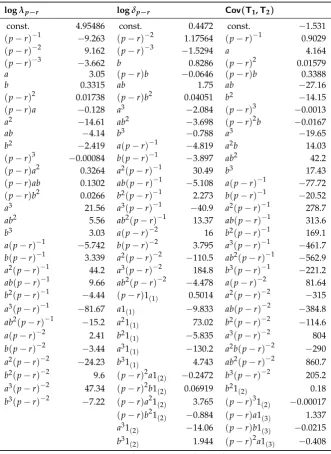
Performing a series of regression analyses and carefully removing insignificant explanatory variables by utilising theAutometrics option available inPcGive(Doornik and Hendry 2013), we arrived at parsimonious response–surface functions for logλp−r, logδp−randCov(T1,T2); these functions are henceforth denoted fpz−r(p−r,a,b,T)withztaking valuesλ,δandcov, respectively.
TablesA1andA2in AppendixArecord the rounded coefficients fora,b,p−rand their variants in the response surface regression for the broken linear trend case and the broken constant case, respectively. The inverse of the observation number,T−1, and its variants such asT−2, also play critical roles in the response surface regression, but all of them are irrelevant asymptotically and thus disregarded when calculating the limit approximates based on these tables.
It should also be noted that a response–surface regression analysis ofCov(T1,T2)was technically difficult in terms of residual diagnostic tests. Doornik (1998) used the average of estimates for Cov(T1,T2)when performing a response surface analysis for partial systems with no break. We adhered to the regression approach, rather than simply taking the average of the covariance estimates, by assigning importance to various significant influences of a, b and p−r on the behaviour of Cov(T1,T2). This regression analysis indeed bore fruit and clarified the highly complex structure of the dependence ofCov(T1,T2)ona,b,p−rand its variants, as shown in the third column of each of TablesA1andA2. These findings aboutCov(T1,T2)are not known in the literature, thus giving added value to the response surface study conducted in this paper, although the impact of variation in Cov(T1,T2)on the approximate shape and scale parameters may not always be large.
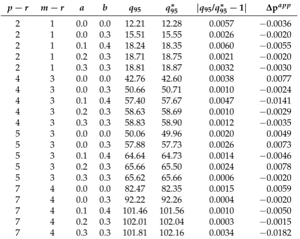
Tables1and2display a set of examples demonstrating the accuracy of the response surface regression results. A class of approximately 95% limit quantiles is presented in each of the tables for various combinations ofa,b,p−randm−r, when either broken-linear-trend or broken-constant specifications are adopted in analysis. Approximate quantiles in the fifth column (q95) in Tables1and2
are derived from TablesA1andA2, respectively; that is, they are from the full-system-based response surface analysis, combined with the mappings (29), (30) and (31). By contrast, approximate quantiles recorded in the sixth column (q∗95) of each table, except those fora=b =0, were obtained directly from auxiliary response surface regressions based on partial-system simulations with the sameTs andNas above. Each of these auxiliary regression equations employed a simulated 95% quantile as a response variable and involved a constant,T−1and its powers if necessary, as explanatory variables. The regression equations vary in specification for the purpose of capturing the underlying smooth response surfaces of various simulated quantiles; the graph of each regression’s actual and fitted values was checked to ensure the capturing of the underlying smoothness. Estimated constants in these regression equations are recorded in the columns forq∗95as approximate 95% limit quantiles. The limit quantiles inq95∗ fora=b=0 (that is, no break cases) were taken from Doornik(2003).
Tables1and2show that the quantiles in q95 almost coincide with those inq∗95 regardless of specifications of the deterministic terms; see the seventh column of each table for
q95/q∗95−1
, a series of absolute relative errors, all of which are very small. This correspondence can be seen as strong evidence supporting the validity of the proposed approximation method based on the full model. Furthermore, the eighth column of each table records a class of discrepancies in approximatep-values, defined as∆papp=g q95
q95−q∗
95
, in whichg(·)represents a gamma density function calculated from simulated mean and variance. Most of the discrepancies are very small, and even the largest one is around 0.02 whenp−ris relatively large, for which we should recall that a large value ofp−r could give rise to various other distortion issues in practice. The overall evidence allows us to argue that the approximate quantiles work as useful critical values in applications from a practical viewpoint. The Supplementary Materials includes an Ox code for simulating asymptic distribution. This can be used if further precision is needed.
dimension may require careful examinations of the underlying cointegrating rank, in addition to the application of the proposedPLRtests to the data under study, as discussed byJuselius(2006, §8).
Table 1.A comparative analysis of 95% limit quantiles: broken linear-trend models.
p−r m−r a b q95 q95∗ |q95/q∗95−1| ∆papp
2 1 0.0 0.0 15.45 15.33 0.0078 0.0058
2 1 0.0 0.3 21.25 21.25 0.0000 0.0000
2 1 0.1 0.4 25.63 25.76 0.0050 −0.0065
2 1 0.2 0.3 27.23 27.11 0.0044 0.0055
2 1 0.3 0.3 27.74 27.62 0.0043 0.0056
4 3 0.0 0.0 50.29 50.08 0.0042 0.0100
4 3 0.0 0.3 65.09 64.97 0.0018 0.0057
4 3 0.1 0.4 77.01 76.84 0.0022 0.0082
4 3 0.2 0.3 80.25 80.11 0.0017 0.0068
4 3 0.3 0.3 81.92 81.84 0.0010 0.0039
5 3 0.0 0.0 57.35 57.32 0.0005 0.0015
5 3 0.0 0.3 72.27 72.03 0.0033 0.0112
5 3 0.1 0.4 84.00 83.98 0.0002 0.0010
5 3 0.2 0.3 87.23 87.10 0.0015 0.0063
5 3 0.3 0.3 88.44 88.47 0.0003 −0.0015
7 4 0.0 0.0 91.64 91.79 0.0016 −0.0077
7 4 0.0 0.3 110.97 110.81 0.0014 0.0076
7 4 0.1 0.4 126.33 126.34 0.0001 −0.0005
7 4 0.2 0.3 130.53 130.07 0.0035 0.0215
7 4 0.3 0.3 131.26 131.45 0.0014 −0.0097
Notes.q95denotes 95% limit quantiles approximated from the full systems, whileq∗95denotes those calculated
directly from the partial systems.∆papprepresents discrepancies in approximatep-values.
Table 2.A comparative analysis of 95% limit quantiles: broken constant models.
p−r m−r a b q95 q95∗ |q95/q∗95−1| ∆papp
2 1 0.0 0.0 12.21 12.28 0.0057 −0.0036
2 1 0.0 0.3 15.51 15.55 0.0026 −0.0020
2 1 0.1 0.4 18.24 18.35 0.0060 −0.0055
2 1 0.2 0.3 18.71 18.75 0.0021 −0.0020
2 1 0.3 0.3 18.81 18.87 0.0032 −0.0030
4 3 0.0 0.0 42.76 42.60 0.0038 0.0077
4 3 0.0 0.3 50.66 50.71 0.0010 −0.0024
4 3 0.1 0.4 57.40 57.67 0.0047 −0.0141
4 3 0.2 0.3 58.63 58.69 0.0010 −0.0029
4 3 0.3 0.3 58.83 58.90 0.0012 −0.0035
5 3 0.0 0.0 50.06 49.96 0.0020 0.0049
5 3 0.0 0.3 57.88 57.73 0.0026 0.0073
5 3 0.1 0.4 64.64 64.73 0.0014 −0.0046
5 3 0.2 0.3 65.66 65.50 0.0024 0.0078
5 3 0.3 0.3 65.62 65.66 0.0006 −0.0020
7 4 0.0 0.0 82.47 82.35 0.0015 0.0059
7 4 0.0 0.3 92.22 92.26 0.0004 −0.0020
7 4 0.1 0.4 101.46 101.56 0.0010 −0.0050
7 4 0.2 0.3 102.01 102.04 0.0003 −0.0015
7 4 0.3 0.3 101.81 102.16 0.0034 −0.0182
Notes.q95denotes 95% limit quantiles approximated from the full systems, whileq∗95denotes those calculated
directly from the partial systems.∆papprepresents discrepancies in approximatep-values.
4.2. Implementation of Response Surface
In the case ofq=3 sample periods and thus 2 breaks atT1,T2, where 0<T1<T2<T, we leta,b be the smallest and second-smallest relative sub-sample length. Thus, ifv1=T1/T,v2= (T2−T1)/T, v3= (T−T2)/Tso thatv1+v2+v3=1. We choosea=min(v1,v2,v3)andb=median(v1,v2,v3).
In the case ofq = 2 sample periods and thus 1 break atT1, where 0 < T1 <, thenv1 = T1/T, v2= (T−T1)/T, so thatv1+v2=1. We leta=0 andb=min(v1,v2).
In the case ofq=1 sample period and thus no break, leta=b=0. Theorem4and (28) show that the mean and variance for the cases whereq<3 can be found from those forq=3 by choosinga,bas indicated and subtracting(3−q)(p−r)and 2(3−q)(p−r), respectively.
Given the choices ofp−r,m−r,aandb, compute the approximations to
fλ
p−r =logλp−r, fpδ−r =logδp−r, cp−r =Cov(T1,T2). (32) TableA1is used for the case with a broken linear trend while TableA2is used for the case with a broken constant. This is then inserted in (31), which in turn is inserted into (29), (30), while correcting for the number of breaks, that is,
E( m−r
∑
i=1
Ti) = m−r p−r exp(f
δ
p−r+fpλ−r)−(3−q)(m−r), (33)
Var( m−r
∑
i=1
Ti) = m−r
p−r exp(2f δ
p−r+fpλ−r)−(m−r)(p−m)cp−r−2(3−q)(m−r). (34)
Finally, we approximate the quantile of interest or thep-value of the observedPLRstatistic using a gamma distribution with mean and variance matching (33) and (34). Equivalently, one can specify the shape and scale of the gamma distribution asmean2/varianceandvariance/mean.
A spreadsheet for implementing the response surfaces in TablesA1andA2is available in the Supplementary Materials. This also includes an Ox program for simulating the asymptotic distributions and calculating p-values of observed test statistics for specifications outside the range covered by TablesA1andA2, for instance when the number of structural breaks is greater than 2 orq>3.
5. Empirical Illustration
As empirical illustration, we analyse a set of quarterly time series data fromSchreiber(2015), who attained an econometric system for the exchange rate and bilateral trade between the UK and Germany. She decomposed the UK-Germany economic system into two blocks, a foreign exchange block and bilateral trade block, in order to obtain a data-congruent representation useful for forecasting and policy analysis. Various econometric studies were conducted bySchreiber(2015), and one of them was the analysis of a partial model for the bilateral trade block with a structural break. The methodology developed in the above sections enables us to conduct formal tests for cointegrating rank that underlies such a partial system subject to a break. This partial system analysis may also be encouraged in terms of local power advantage of partial-system-based tests over those based on a full system under weak exogeneity, as demonstrated by Doornik et al.(1998) as well asKurita(2011).
1990 1995 2000 2005 2010 2015 −0.8
−0.6 −0.4 −0.2
(a)
tb
1990 1995 2000 2005 2010 2015 −0.2
0.0 0.2 0.4
(b) ∆ulc
1990 1995 2000 2005 2010 2015 5.75
6.00 6.25 6.50
(c)
y y*
1990 1995 2000 2005 2010 2015 0.0
0.1
0.2 (d)
ppp
Figure 1.Data. (a)tbtis the trade balance between the UK and Germany; (b)dulctis the unit labour
cost differential between the UK and Germany; (c)ytandy∗t are the logs of the UK and German gross
domestic products, respectively; (d)ppptis the terms of trade.
In this empirical illustration, we analyse the data using a bivariate partial autoregressive model fortbtanddulct, withyt,y∗t andppptassumed to be weakly exogenous for the class of parameters of interest such as cointegrating vectors; that is,p=5 andm=2. This assumption is based on Schreiber’s study, suggesting that modelling the bilateral trade block centering ontbtanddulctappears to be conformable to the underlying data structure. The lag-lengthk=2 is selected for our bivariate partial autoregressive model.
With regard to the issue on a structural break, we adopt a broken trend specification; that is, the presence of a shift in the restricted trend as well as the unrestricted constant. The second sub-sample period starts in 2008.3, corresponding to the observation point inTq−1forq=2, which results in the selection of relative break pointsa= 0 andb=0.255. According to (10), our bivariate model with k=2 requires a set of two impulse dummy variables for the initial values of the second sub-sample periods. In addition, a pair of impulse dummy variables,Dp1998(1)andDp2006(2), is employed in our model to capture outliers in the data, as inSchreiber(2015); the former variable is 1 in 1998.1 and zero otherwise for an outlier due to the Asian financial crisis, while the latter is 1 in 2006.2 and zero otherwise, corresponding to an outlier attributable to an increase in oil prices.
Table 3.Diagnostic test statistics for the estimated partial system.
Single-Eq. Tests tbt dulct Vector Tests
FAR5(5,66) 0.946[0.457] 0.777[0.570] FAR5(20,120) 0.542[0.943] FARCH4(4,84) 0.469[0.758] 0.511[0.728] FHET(93,162) 0.838[0.825]
FHET(31,56) 0.726[0.831] 1.016[0.468] χ2ND(4) 2.233[0.693] χ2ND(2) 1.341[0.512] 0.426[0.808]
Notes.Figures in square brackets arep-values.
Table4presents a class ofPLRtest statistics for the determination of cointegrating rank, along with the correspondingp-values and approximate 95% limit quantiles calculated from the response surface outcomes in the previous section. We used TableA1 in AppendixAto calculate approximates to logδp−r, logλp−randCov(T1,T2), and then applied them to the mappings (29) and (30) adjusted for extraχ2terms, so that the gamma-distribution approximation method yielded thep-values. Table4 shows that, at the 5% level, the null hypothesisr=0 is rejected while the hypothesisr≤1 fails to be rejected. Hence, this formal analysis enables us to reach the conclusion ofr=1, which supports the informal analysis ofSchreiber(2015).
Table 4.Testing for cointegrating rank.
r=0 r≤1
PLR{H`(r)|H`(2)} 56.610[0.014]∗ 21.964[0.148] 95% limit quantiles 50.864 26.334
Notes.Figures in square brackets arep-values.∗denotes significance at the 5% level.
The estimated cointegrating relationship under some additional restrictions is
tb= 0.259
(0.121)dulct−0.726(0.3)pppt+(2.340.323)(y
∗
t −yt)−0.019
(0.004)t1(≥2009:1)+υt, (35)
where a figure in brackets under each coefficient is a standard error and υt is a stationary error. The signs of the coefficients in (35) are the same as those inSchreiber(2015)’s cointegrating equation except fory∗t. The German incomey∗t was insignificant in her cointegrating relationship and thus removed from it, while, in (35),y∗t plays a significant role, along withyt. As a result of checking a set of unrestricted estimates for the cointegrating vector, we have arrived at Equation (35), where the coefficients ofytandy∗t are restricted to add to zero, while a zero-restriction is placed on the coefficient fort1(≤2008:2); that is, a linear trend is present only in the second sub-sample period. The PLRtest
statistic for these restrictions is 3.571[0.168], in which the figure in square brackets is ap-value according toχ2(2). Thus, the hypothesis of the overall restrictions cannot be rejected at the 5% level.
There are several interesting aspects of Equation (35) that are worth discussing here. The real income difference between Germany and the UK,y∗t −yt, has a positive coefficient, implying that a spread in the income difference leads to an improvement in the UK trade balance with Germany. This finding is interpretable in the context of an income effect from each of the two countries. The coefficient for the terms of trade, pppt, should also be noted. It is negative, thus indicating a relative price effect on the trade balance in a theory-consistent manner; that is, a decrease in exports prices relative to import prices leads to trade balance improvement, so that the well-known elasticity approach to trade balance appears to be empirically valid for the two countries. Furthermore, the linear trendtis significant solely in the second sub-sample period, suggesting long-lasting influences of the global recession on the two countries’ trade balance and other economic variables.
Finally, we will check that the three variables,yt,y∗t andpppt, are indeed weakly exogenous for the class of parameters of interest. We follow the testing procedure suggested byJohansen(1992a),
test for the significance of the cointegrating combination in each equation. Table5reports a class of LRtest statistics for the exclusion of the empirical cointegrating linkage from each equation in the marginal system. Judging from the reportedp-values according toχ2(1), none of the test statistics indicate evidence against the assumption of weak exogeneity; thus, the preceding partial-system analysis of cointegrating rank has been justified.
Table 5.Checking weak exogeneity.
yt y∗t pppt
0.004[0.951] 1.183[0.277] 1.954[0.162]
Notes.Figures in square brackets arep-values.
6. Conclusions
This study has explored partial cointegrated vector autoregressive models subject to structural breaks in deterministic terms, a linear trend and constant. The Granger–Johansen representation of the full model in JMN has been reexamined, leading to a useful clarification of roles of the initial values in asymptotic analysis. A class of log likelihood ratio test statistics for cointegrating rank has then been introduced in the proposed partial-model framework. We have investigated asymptotic theory under a general class of innovation distributions allowing martingale difference sequences with conditional heteroscedasticity. The derived limit distributions of the statistics are closely related to those for the full models investigated by JMN. This relationship allows us to perform a response surface analysis in a simplified full-system framework, instead of relying on laborious partial-system-based simulations. The outcomes of the analysis are summarised as a set of two statistical tables providing valuable information for inference on the underlying cointegrating rank. Lastly, an empirical analysis of real-life data from the UK and Germany has demonstrated the practicality of these tables in applied economic research. As a result of this study, the partial cointegrated models have become more flexible and reliable devices for modelling time series data subject to various structural breaks.
Recently, bootstrap methods have been proposed for cointegration rank testing in full systems (Cavaliere et al. 2012). It would be interesting to extend those to partial systems with or without breaks.
Supplementary Materials:The following are available online athttp://www.mdpi.com/2225-1146/7/4/42/s1: A preadsheet for implementing the response surface in TablesA1andA2, as well as an Ox program for simulating the asymptotic distributions.
Author Contributions:The authors made equal contributions.
Funding:T. Kurita gratefully acknowledges financial support for this work from JSPS KAKENHI (Grant Nos: 15KK0141 and 26380349).
Acknowledgments: We are grateful to the editors and two anonymous referees for constructive comments. The results reported in this paper were presented at Norwegian University of Science and Technology (NTNU), Statistics Norway and the University of Copenhagen. We would like to thank Gunnar Bårdsen, Pål Boug, Søren Johansen and various other seminar participants for helpful comments and suggestions.
Appendix A. Tables for Response Surfaces
Table A1.Response surfaces for broken trend models.
logλp−r logδp−r Cov(T1,T2)
const. 4.14 const. 0.5987 const. −1.298
(p−r)−1 −6.301 p−r −0.0538 1(2) 0.03616
(p−r)−2 5.8842 a −1.039 1(4) −0.027
(p−r)−3 −2.32576 b −0.39 (p−r)−3 −2.022
p−r 0.17 (p−r)2 0.00686 a −8.689
a 2.6165 a2 5.547 b 2.225
b 2.5245 ab 2.331 a2 59.77
(p−r)a −0.0572 b2 1.841 ab 24.31
(p−r)b −0.0971 (p−r)3 −0.00033 b2 −5.156
a2 −7.550 a3 −10.42 a3 −133.5
ab −5.323 ab2 −4.325 ab2 −59.05
b2 −7.412 b3 −2.553 a(p−r)−1 −29.55
(p−r)3 −0.000124 a(p−r)−1 9.905 b(p−r)−1 −66.58 (p−r)ab 0.161 b(p−r)−1 1.862 b2(p−r)−1
255.3 (p−r)b2 0.179 a2(p−r)−1 −61.09 a3(p−r)−1 280.5 a3 10.40 ab(p−r)−1 −17.09 ab2(p−r)−1 155.3 ab2 6.096 b2(p−r)−1 −11.48 b3(p−r)−1 −240 b3 5.851 a3(p−r)−1 117.68 a(p−r)−2 21.32 a(p−r)−1 −8.860 ab2(p−r)−1 35.19 b(p−r)−2 71.68 b(p−r)−1 −4.948 b3(p−r)−1 18.6 b2(p−r)−2 −305.7 a2(p−r)−1
46.15 a(p−r)−2 −8.836 a2b(p−r)−2 −321.1 ab(p−r)−1 31.85 b(p−r)−2 1.033 b3(p−r)−2 332.1 b2(p−r)−1 26.12 a2(p−r)−2 66.94 (p−r)1(3) 0.038 a3(p−r)−1 −86.58 ab(p−r)−2 10.84 b21(3) −0.184 ab2(p−r)−1 −50.50 a3(p−r)−2 −140.88
b3(p−r)−1 −28.78 ab2(p−r)−2 −30.16 a(p−r)−2 5.296 b3(p−r)−2 −10.05
b(p−r)−2 2.386 a1(1) 2.107
a2(p−r)−2 −29.03 b1
(1) −1.029
ab(p−r)−2 −19.46 a21
(1) −20.63
b2(p−r)−2 −13.42 b21
(1) 3.511
a3(p−r)−2 62.00 a31
(1) 45.85
a2b(p−r)−2 −5.880 ab21(1) 4.267 ab2(p−r)−2 34.59 (p−r)b21(2) 0.062 b3(p−r)−2 15.93