www.the-cryosphere.net/10/2953/2016/ doi:10.5194/tc-10-2953-2016
© Author(s) 2016. CC Attribution 3.0 License.
Improved retrieval of land ice topography from CryoSat-2 data and
its impact for volume-change estimation of the Greenland Ice Sheet
Johan Nilsson1, Alex Gardner1, Louise Sandberg Sørensen2, and Rene Forsberg2 1Jet Propulsion Laboratory, California Institute of Technology, Pasadena, CA 91109, USA
2DTU Space, National Space Institute, Technical University of Denmark, 2800 Kgs. Lyngby, Denmark
Correspondence to:Johan Nilsson ([email protected])
Received: 4 May 2016 – Published in The Cryosphere Discuss.: 6 June 2016
Revised: 18 October 2016 – Accepted: 19 October 2016 – Published: 1 December 2016
Abstract.A new methodology for retrieval of glacier and ice sheet elevations and elevation changes from CryoSat-2 data is presented. Surface elevations and elevation changes deter-mined using this approach show significant improvements over ESA’s publicly available CryoSat-2 elevation product (L2 Baseline-B). The results are compared to near-coincident airborne laser altimetry from NASA’s Operation IceBridge and seasonal height amplitudes from the Ice, Cloud, and El-evation Satellite (ICESat).
Applying this methodology to CryoSat-2 data collected in interferometric synthetic aperture mode (SIN) over the high-relief regions of the Greenland Ice Sheet we find an im-provement in the root-mean-square error (RMSE) of 27 and 40 % compared to ESA’s L2 product in the derived eleva-tion and elevaeleva-tion changes, respectively. In the interior part of the ice sheet, where CryoSat-2 operates in low-resolution mode (LRM), we find an improvement in the RMSE of 68 and 55 % in the derived elevation and elevation changes, re-spectively. There is also an 86 % improvement in the mag-nitude of the seasonal amplitudes when compared to am-plitudes derived from ICESat data. These results indicate that the new methodology provides improved tracking of the snow/ice surface with lower sensitivity to changes in near-surface dielectric properties.
To demonstrate the utility of the new processing method-ology we produce elevations, elevation changes, and total volume changes from CryoSat-2 data for the Greenland Ice Sheet during the period January 2011 to January 2015. We find that the Greenland Ice Sheet decreased in volume at a rate of 289±20 km3a−1, with high interannual variabil-ity and spatial heterogenevariabil-ity in rates of loss. This rate is
65 km3a−1more negative than rates determined from ESA’s L2 product, highlighting the importance of CryoSat-2 pro-cessing methodologies.
1 Introduction
In April 2010, the European Space Agency (ESA) launched CryoSat-2 tasked with monitoring the changes of the Earth’s land and sea ice. CryoSat-2 carries a new type of de-lay/Doppler radar altimeter (Raney, 1998) referred to as SIRAL (SAR Interferometric Radar Altimeter). SIRAL op-erates in two different modes over land ice. Over the in-terior part of the ice sheets it operates as a conventional pulse limited radar system, referred to as the low-resolution mode (LRM). In more complex high-sloping terrain the sys-tem uses a second antenna to operate in interferometric syn-thetic aperture radar (SIN) mode. This new feature allows the satellite to monitor changes in complex terrain, includ-ing ice caps, glaciers, and the high-relief marginal areas of the ice sheets. Such areas are sensitive to changes in climate and contribute greatly to current rates of sea level rise (e.g., Gardner et al., 2013; Shepherd et al., 2012).
conditions can introduce time-varying biases in the data that, in combination with the radar signals interaction with the sur-face, introduce large elevation biases (0.5–1 m) (Nilsson et al., 2015a). This, combined with other factors such as pro-cessing methodology and surface topography, makes it dif-ficult to measure small changes for much of the word’s ice-covered regions (Arthern et al., 2001; Gray et al., 2015; Nils-son et al., 2015b).
The mitigation of these effects in the processing of radar altimetry data is required for improved accuracy of derived temporal and spatial changes in surface elevation of glaciers and ice sheets. Several studies have proposed different ap-proaches to assess these effects and improve the retrieval pro-cess of surface elevation and elevation changes from radar al-timetry data. These include different approaches to waveform retracking (Davis, 1993, 1997; Gray et al., 2015; Helm et al., 2014) and empirical corrections to the estimated surface elevation changes (Davis and Ferguson, 2004; Flament and Rémy, 2012; Sørensen et al., 2015; Wingham et al., 2006b; Zwally et al., 2005, 2011). Relatively little work has been done to assess methods for improving elevation and elevation changes derived from ESA’s CryoSat-2 data (Abulaitijiang et al., 2015; Gray et al., 2013, 2015; Helm et al., 2014).
Here we conduct a thorough analysis of CryoSat-2 SIN and LRM waveform retracking, filtering and processing methodologies to design an optimal processing methodol-ogy for CryoSat-2 elevation retrieval over both smooth and complex ice-covered terrain. We then analyze two differ-ent approaches in determining surface elevation and volume changes from the scattered CryoSat-2 elevation retrievals. The overarching goal of this work is to develop robust and accurate elevation retrieval algorithms that are less sensitive to changes in surface and subsurface scattering properties.
The new processing scheme is applied to estimate eleva-tion and volume changes of the Greenland Ice Sheet for the period January 2011 to January 2015, using two indepen-dent methods to characterize the differences of the results due to methodology. The results are compared to change es-timates obtained from the ESA L2 Baseline-B surface eleva-tion product (Bouzinac et al., 2014), high-accuracy airborne data from NASA IceBridge Airborne Topographic Mapper, and seasonal height amplitudes estimated from Ice, Cloud, and Elevation Satellite (ICESat) data.
2 Surface elevations from CryoSat-2 2.1 Low-resolution mode (LRM)
The LRM data is used over the interior parts of the ice sheet, which mostly consist of low-sloping terrain. Here, SIRAL operates as a conventional pulse-limited radar system with a transmission frequency of 13.6 GHz (Ku-band) and has a pulse-limited footprint (PLF) radius of approximately 1.5 km and a beam-limited footprint (BLF) radius of approximately
7.5 km over flat terrain (Bouzinac, 2014). The gentle ter-rain allows for accurate mapping of the surface elevation of the ice sheet down to decimeter-level (Brenner et al., 2007). Within the LRM waveform we define the location of the sur-face from the leading edge of the waveform based on a frac-tion of the maximum amplitude of the received power. This approach is commonly referred to as a threshold retracker. Following Davis (1997) we use a 20 % threshold to define the location of the surface. Davis (1997) argued that a 20 % threshold represents the best compromise between wave-forms that are entirely dominated by either volume or sur-face scattering, making it suitable for obtaining estimates of surface elevation for most parts of the Greenland Ice Sheet.
The CryoSat-2 LRM radar waveforms suffer from mea-surement noise, in the form of speckle noise. Furthermore, over the steeper parts of the LRM area the range gate track-ing loop can lose track of the surface, productrack-ing unusable waveforms. To remove bad or loss-of-track waveforms the radar waveform (20 Hz) is first filtered using a zero-phase low-pass filter to reduce speckle noise on a line-by-line ba-sis. The signal-to-noise ratio (SNR) of the waveform is then estimated and if the SNR<0.5 dB the waveform is rejected. The SNR threshold was empirically chosen to obtain a good trade-off between the quality of the measurements and sam-pling.
Before the waveform can be retracked the first surface re-turn (first major peak) is identified within the range gate win-dow. A copy of the waveform is heavily smoothed to remove small-scale surface roughness signals, keeping the overall surface signal intact. The range gate index of the first peak from the copy is then used to extract the leading edge of the original low-pass filtered waveform. Only leading edges with a peak index above 20 are used in the retracking, as peaks before that can indicate troublesome surface ranging. The extracted leading edge is then oversampled by a factor of 100 (cf. Gray et al., 2013; Helm et al., 2014), and the range
R between the surface and satellite is determined based on the 20 % threshold computed according to Davis (1997). The range is then corrected for several atmospheric and geophys-ical effects relevant to land ice studies according to Bouzinac (2014). The surface elevationH of the topography, relative to the WGS84 ellipsoid, is estimated asH=A−R, where
Ais the altitude of the satellite.
Remy et al. (1989) showed that accounting for surface cur-vature in addition to surface slope significantly improves re-sults. The surface slope, aspect, and curvature are estimated from an a priori DEM. The GIMP elevation model (Howat et al., 2014) was used to derive surface parameters for the slope-induced error correction in the LRM data. The DEM was resampled to 2 km resolution, using bilinear interpola-tion prior to parameter estimainterpola-tion, which provided the lowest root-mean-square error and further corresponds to the pulse-limited footprint of the LRM data.
2.2 Interferometric synthetic aperture radar (SIN) mode
The SIN mode is used over the marginal areas of the ice sheets and other smaller glacier-iced areas. In these areas the SIRAL altimeter operates as a delay/Doppler radar system (Raney, 1998). The delay/Doppler radar allows for higher along-track resolution compared to conventional altimetry, resulting in 350 m resolution in along track and 1500 m across track. In ordinary SAR operation only the amplitude of the radar echo is measured and the phase content is dis-carded or ignored. With the inclusion of a second antenna on CryoSat-2, interferometric SAR can be performed. The dif-ference in path length between the POCA and the individual antennas introduces a phase shift between the two retrieved signals that can be related to the angle of arrival (look angle). The look angle can in turn be used to resolve the across-track (across-antenna) location of the echo.
Multi-look processing is applied to ESA’s L1B waveform product (Bouzinac, 2014) to reduce the noise in the SIN waveform but it is still affected by speckle noise, as is the case for the LRM waveforms. To mitigate this effect, and to help identify the leading edge of the first return, we apply speckle reduction filtering and leading edge extraction of the SIN waveforms in the same way as for the LRM data pro-cessing, with minor changes due to differences in range gate resolution. In this case, compared to the LRM retracking al-gorithm, only leading edges with a peak index in the range of 100–350 are used for retracking the radar waveform (Pw). The estimated coherenceCof the multi-looked waveforms is then filtered in two stages: (i) all coherence measurements larger than one are set to zeros (coherence values larger than one exists in the L1B product due to unknown reasons); (ii) the coherence array, as a function of range, is filtered us-ing a 2-D 5×5 Wiener filter to remove high-frequency noise. The filtering of the waveform and the coherence is applied to remove noise in the recreation of the interferogram, dis-cussed below.
The measured differential phase φof the return signal is affected by phase ambiguities, for example, a sudden shift of 2πin the measured phase. To reduce phase noise and aid the phase, an unwrapping of the radar interferogramI is
per-formed according to Gray et al. (2013):
I=Pw·C·e−iφ. (1) The interferogram is then filtered using a wavelet-based de-noising technique, where the real and imaginary parts of the interferogram are filtered separately. The unwrapping of the interferogram allows for indirect filtering of the phase without being affected by the phase ambiguities. Phase fil-tering is an important consideration as it has a direct ef-fect on accuracy of the position of the ground echo. We se-lected a bi-orthogonal wavelet as the mother wavelet to pro-duce the wavelet coefficients decomposed into three levels. Soft thresholding was applied to detail coefficients, using a heuristic threshold rule to remove noise at every level. This was done on a line-by-line basis. The final filtered differen-tial phase was then recovered by
φf=6 IfRe+j·I Im f
, (2)
whereIfReis the real part of the interferogram andIfImis the imaginary part. To resolve the phase ambiguities the filtered phase measurements require unwrapping. The phase unwrap-ping is done on a line-by-line basis in two directions start-ing from the center of gravity of the waveform (Wstart-ingham et al., 1986).
The return power distribution of a delay/Doppler radar system shows an important distinction from those from con-ventional pulse-limited radar systems. Here, the point cor-responding to the mean surface is not located at the half-power point on the leading edge, but rather closer to the max-imum (Wingham et al., 2006a). Therefore, a new retracker has been developed, closely related to the one used in Gray et al. (2013), to allow for adaptive retracking of the upper parts of the leading edge of the SAR waveform. The algorithm follows the main concept of the threshold retracker, devel-oped by Davis (1997), but instead of a pre-defined thresh-old it tracks the maximum gradient of the leading edge of the oversampled waveform. We refer to this approach as the “leading-edge maximum gradient retracker” (LMG).
The surface returns are geolocated using the across-track look-angleθestimated from the differential phase at the re-tracking point according to Wingham et al. (2006a). This, in combination with the viewing geometry, is used to define the location of the surface return on the ground using basic across-track interferometric principles. We correctθ for the interferometer surface slope error by applying the look-angle scaling factor estimated in Galin et al. (2013) and for the plat-form roll angle.
come from a position upslope from the nadir point. There-fore the following relation must hold where (Hecho> Hnadir) or for a more practical application(Hecho−Hnadir) > εDEM, whereεDEMis the uncertainty of the DEM used. If this re-lation is violated 2πis added or subtracted to the individual along-track phase estimate, depending on the sign.
A final step is applied to correct for any lingering phase ambiguities not corrected by the a priori DEM. This step uses the assumption that the along-track phase should follow a consistent pattern over most of the satellite ground track. Hence, any large discrepancies from the overall pattern of the along-track phase would indicate an ambiguity. The am-biguity is detected by computing the residuals of the along-track phase by removing a smoothed version of the differ-ential phase. If any of the residuals have a magnitude larger thanπthey are considered ambiguous and thus corrected by adding or subtracting 2π.
3 Surface elevation changes from CryoSat-2 3.1 Surface-fit method
The surface-fitting method (SF) is based on fitting a linear model to the elevations as a function of time and space inside a search radius of 1 km (e.g., Howat et al., 2008; Moholdt et al., 2010; Sørensen et al., 2011; Wouters et al., 2015). The linear model consists of a time-invariant (static) bi-quadratic surface model to account for variable topography inside the search radius and a time-variant part used to extract the tem-poral change in elevation. The model consists of a total of seven parameters, where six of the parameters (a coeffi-cients) describe the bi-quadratic surface-modeling function,
∂h/∂t the linear elevation change rate, t time in decimal years,t0the mean time inside the footprint, andεthe residu-als from the linear regression.
h (x, y, t )=a0+a1x+a2y+a3xy+a4x2+a5y2 +∂h
∂t(t−t0)+ε (3)
The algorithm estimates the elevation change at every echolocation (or grid node if desired) in the data set. In each solution the signal amplitude and phase are also estimated by fitting a seasonal signal model to the surface-fit elevation residuals, according to
1h (t )=s0cos(2π t )+s1sin(2π t )+ε, (4) where 1h is the elevation residuals estimated from the surface-fit model, s0,1 are the model coefficients, and t is the time. The amplitudeAis then defined asA=
q
s02+s21
and the phaseP asP =tan−1s1
s0
.
To remove outliers an iterative 3σ filter is used in the full model solution i.e., the topography, trend, and seasonal sig-nal are removed, using a maximum of five iterations. For
each iteration residuals (full-model) with an absolute value larger than 10 m are removed, as seasonal changes larger than 10 m are not expected (Moholdt et al., 2010; Qi and Braun, 2013). The data inside the 1 km cap are weighted according to their distance from the estimation point according to
W= 1
1+d ρ
2, (5)
whereW is the estimated weight,d the distance, andρ the correlation or resolution parameter set to 500 m. The weight-ing allows the solution to better reflect local signal dynamics at the prediction point.
Local elevation time series are further computed from the elevation residuals and elevation trend for each solution ac-cording to
h (x, y, t )=∂h
∂t (t−t0)+ε, (6)
wheret is the time epochs inside the search cap, t0 is the mean time oft,∂h/∂tis the estimated elevation change rate, andεis the elevation residual at each time epoch.
The elevation changes estimated from the surface-fitting method are then culled to remove outliers before spatial grid-ding. Elevation changes with an absolute trend larger than 15 m a−1 are removed. The resulting surface elevations are binned at 5 km resolution for outlier-editing purposes. For each cell the local spatial trend is modeled as a bilinear sur-face, and removed. The residuals are then edited using an it-erative 3σ filter until the RMS (root mean square error) con-verges to 2 %.
3.2 Crossover method
The crossover method is used to derive the surface eleva-tions at the intersection point between an ascending and de-scending satellite ground track separated in time (Brenner et al., 2007; Khvorostovsky, 2012; Zwally et al., 1989). The sur-face elevations and times are then estimated at the crossover location for each track by linear interpolation of the two clos-est data points for each ascending and descending track. The crossover height difference is then estimated by taking the height difference between the two tracks according to
1h=h2−h1+ε, (7) whereh1andh2are the surface heights at the crossover loca-tion at time epocht1andt2, respectively, andεis the random measurement error, including orbital, range, and retracking errors.
This produces annual and sub-annual crossover difference around each crossover location. This fact is used to produce elevation change rates by incorporating all multi-temporal crossover difference within a neighborhood of 2.5 km around each crossover location. The elevation change is then esti-mated using the same procedure described for the surface-fit method, except that a bilinear model is used to remove any spatial trends in the topography of the crossover elevations according to
dh(x, y, t )=a1x+a2y+
∂h
∂t(t−t0)+ε, (8)
where dhis the crossover height difference,t the time,t0the mean reference time inside the footprint,a1anda2the across and along-track slope, and ∂h/∂tthe elevation change rate. This produces elevation changes comparable in time and in spatial coverage with the surface-fit method. The same out-lier editing schemes are applied to the crossover elevation change rates as for the surface-fit method.
3.3 Gridding of sparse elevation and elevation-change data
The gridding is done in a polar-stereographic projection with a latitude of origin at 70◦N, central longitude of 45◦W, and origin at the North Pole, and is referenced against the WGS-84 ellipsoid. The observations derived from the surface-fit and crossover methods are gridded at a resolution of 1 km× 1 km, due to the high spatial sampling.
The method of least squares collocation (LSC), described in Herzfeld (1992), is used to grid the observations onto a regular grid. LSC is similar to Kriging and allows for optimal interpolation and merging of data with different accuracies, using their inherent covariance structure. The LSC algorithm uses the 25 closest data points in 8 quadrants surrounding the prediction point to reduce spatial biasing. The predic-tion equapredic-tion consists of two terms where the first term is the actual prediction term and the second term accounts for the non-stationary part of the data, as described by
ˆ
s=Csz(Czz+N)−1z+
1−X Csz(Czz+N)−1
m (z) , (9) whereCszis the cross-covariance,Czzis the auto-covariance, Nthe diagonal noise matrix consisting of the a priori RMSE, andm(z)is the median value of the observations inside the search neighborhood.
The covariance of the data inside the local neighborhood is modeled as a function of distance away from the prediction point using a third-order Gauss–Markov model described be-low.
C (r)=C0
1+r
α− r2
2α2
e(−αr), (10) wherer is the separation distance,C0is the local data vari-ance, andαis a scaling factor estimated from the correlation length.
LSC interpolation provides a RMSE for each prediction point estimated from the modeled covariance of the data ac-cording to
Csˆ=C0−Csz(Czz+N)−1CTsz, (11) where the RMSE of the prediction equalsσsˆ=(Csˆ)1/2 and CTszis the transposed cross-covariance matrix.
The elevation changes estimated from the surface-fit and crossover methods are interpolated using their a priori er-ror estimated from the regression. To avoid unrealistically small errors, common in the regression errors estimated over flat terrain, a minimum error threshold is applied. Error val-ues smaller than a specific threshold are set to the thresh-old value. The threshthresh-old value is representative of the overall precision of the elevation changes over flat terrain and is set to 0.2 m a−1. The data are then gridded using a 75 km corre-lation length determined from the comparison of CryoSat-2 elevation to airborne measurements (Sect. 5).
The LSC algorithm is also used to generate a DEM based on the surface elevations generated from the surface-fitting algorithm. The surface elevations generated from the surface fit were used as input for the gridding algorithm. The use of surface elevations from the surface fit provides several advantages compared to the raw observations because they provide an almost equal number of observations as the raw data, have been screened for gross outliers, have been low-pass filtered using the 1 km search radius, and all reference roughly the same time epoch. Furthermore, the RMSE gen-erated from the surface-fit-estimated surface height can be used as an a priori error for the LSC gridding procedure.
The DEM is generated using the same approach as for the surface elevation changes, as described previously in this sec-tion, with a correlation length of 25 km. Before the gridding procedure is applied elevationsH <0 andH >3350 m are removed from the data set. Furthermore, elevations with a standard error larger than 30 m are also removed. The eleva-tions are spatially binned into a resolution of 1000 m. Inside each cell the local surface trend is removed by fitting a planar surface, and an iterative 3σfilter is applied to the residuals to remove outliers.
4 Surface elevations and elevation changes from ICESat
al. (2015b). The ICESat elevation, seasonal amplitude, and phase are then used for comparison with CryoSat-2 and to build continuous time series using the surface-fit method de-scribed in Sect. 3.1. For the purpose of this study no correc-tion for the inter-campaign bias was applied, as this is still an active area of investigation.
5 Validation
Elevation and elevation change results were generated for the entire Greenland Ice Sheet using CryoSat-2 data collected between January 2011 and January 2015 using the method-ology presented in Sects. 2 and 3 (JPL product) and by ap-plying the methods of Sect. 3 to ESA’s CryoSat-2 L2 ele-vation products (ESA product). Surface eleele-vations and el-evation changes were validated against airborne data sets collected by NASA’s Operation Ice-Bridge Airborne Topo-graphic Mapper (ATM), obtained from the National Snow and Ice Data Center (NSIDC) in the form of the ILATM2 product. The generated elevation product has a resolution of 80 m, with a 40 m spacing along track. This mission produces both elevation and elevation changes with reported vertical accuracy of∼10 cm and temporal accuracy at the centimeter level (Krabill et al., 2002).
The derived surface elevations from CryoSat-2 are differ-enced against ATM surface elevations within 50 m of each ATM location. One month of CryoSat-2 data consistent in time with the ATM elevations is used for the validation to avoid biases due to temporal sampling and to obtain suffi-cient sample size. A total of 4 years of campaign data is used for the validation of the surface elevations (2011–2014). The residuals are edited using an iterative 3σ filter to remove out-liers. The accuracy and precision is estimated as the mean and standard deviation of the differences, respectively. The residual distribution is further binned according to surface slope estimated from the GIMP DEM (Howat et al., 2014) resampled to 500 m. The sensitivity to surface slope (slope error) can be identified in the standard deviation of the binned residuals and can be used to judge the quality of the produced surface elevation and elevation changes, while the binned average for the elevations can be used to determine radar-signal-penetration depth.
Surface-elevation-change rates estimated from three dif-ferent time periods (2012–2014, 2011–2013, and 2011– 2014) of overlapping ATM observations (Krabill, 2016) are used to validate the surface elevation changes estimated from the CryoSat-2 data. The same validation methodology ap-plied to surface elevations is apap-plied to surface elevation changes, with a few minor modifications. First the search ra-dius is increased to 175 m to make it conform to the ATM elevation-change resolution of 250 m, as this search radius encloses the entire ATM grid cell.
Table 1. Accuracy (Mean), precision (SD), and the total RMSE (RMSE) of surface elevation from CryoSat-2 observations com-pared to IceBridge ATM elevations. Here, the LRM data represent the interior of the ice sheet and SIN the marginal high-relief areas.
Mean (m) SD (m) RMSE (m)
JPL
LRM 0.00 0.43 0.45 SIN −0.52 0.58 0.82
ESA
LRM −1.06 0.89 1.40 SIN −0.90 1.05 1.13
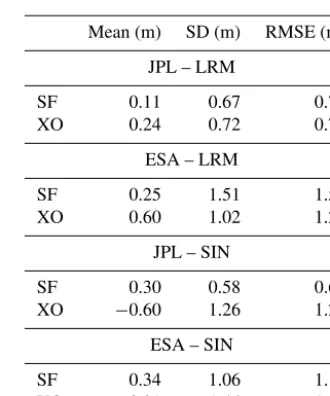
Table 2. Accuracy (Mean), precision (SD), and the total RMSE (RMSE) of surface elevation changes from CryoSat-2 derived from two independent methods (surface fit, SF, and the crossover, XO, methods), compared to IceBridge ATM data. The estimated statis-tics from the elevation change residuals have been multiplied with their individual time intervals.
Mean (m) SD (m) RMSE (m)
JPL – LRM
SF 0.11 0.67 0.70 XO 0.24 0.72 0.78
ESA – LRM
SF 0.25 1.51 1.57 XO 0.60 1.02 1.20
JPL – SIN
SF 0.30 0.58 0.66 XO −0.60 1.26 1.26
ESA – SIN
SF 0.34 1.06 1.11 XO −0.21 1.44 1.44
Secondly the estimated mean and standard deviation are multiplied with the individual time intervals of the validation data sets to make the errors comparable, as they differ in time span.
For the surface-fit and crossover methods, near-coincident elevation change rates were compared with ATM rates (e.g., April 2011 to April 2014). This provided three validation data sets for the surface-fit method due to its high spatial coverage. However, only the 2011–2014 validation data set could be used for the crossover method due to the lower spa-tial sampling of the crossovers.
measurement mode. The weighted average errors for each mode and method are summarized in Tables 1 and 2 for both the ESA and JPL solutions, where the values for the individ-ual campaigns can be found in the Supplement.
For the estimated surface elevation changes from the two independent methods we find the lowest RMSE for the surface-fit method, followed by the crossover method. This differs from the findings of Moholdt et al. (2010), who found lower intrinsic errors for the crossover method compared to the surface-fit method when applied to ICESat data. The larger search radius used for our application of the crossover method most likely explains the difference in findings be-tween the two studies. Furthermore, we find that the surface-fit method provides the largest reduction in RMSE for the JPL product, corresponding to 40 and 55 % for the SIN and LRM data, respectively.
The correlation length used to derive the number of un-correlated grid cells, which is used to estimate the standard error, was determined from a semi-variogram analysis of the elevation-change residuals from CryoSat-2 minus ATM us-ing the data from the surface-fit method. The comparison was done for each mode separately for all the individual campaigns and multiplied with their individual time spans. The semi-variogram was then computed from all the time-invariant residuals for each mode to maximize the spatial coverage. Analysis of the semi-variogram showed approxi-mate correlation lengths of 100 and 75 km for the SIN and LRM data, respectively. These correlation lengths are inside the range of those found by Sørensen et al. (2011) for their analysis of ICESat data, which was found to be between 50 and 150 km.
The main goal of this study is not to derive or compare different types of DEMs. However, to gain insight into the overall quality of our CryoSat-2-derived DEM (referred to as JPL) we compare it to three other DEMs derived from other data sets. First, we compare it to a DEM derived from ESA CryoSat-2 L2 data (referred to as ESA) gridded in the same manner as our DEM (Sect. 3.3). Second we compare it to a DEM from Helm et al. (2014), also based on CryoSat-2 data from CryoSat-2011 to CryoSat-2014 (referred to as AWI). Third, we compare it to a DEM from Howat et al. (2014) (which was used to derive topographical parameters and corrections for the JPL CryoSat-2 data) based on photogrammetry and al-timetry data from the mid 1990s to 2010 (depending on data source) co-registered to ICESat elevation data from 2003 to 2009 (referred to as GIMP).
These data sets were then compared to IceBridge ATM elevations spanning the four different campaigns previously used for validation of the CryoSat-2 elevations. The DEM elevation was estimated at each ATM location using bilinear interpolation, and the elevation difference was computed as (DEM−ATM). No attempt was made to account for differ-ences in DEM and ATM epochs. The estimation of the errors of the DEM was determined in the same way as for the in-dividual CryoSat-2 surface heights. The results of the
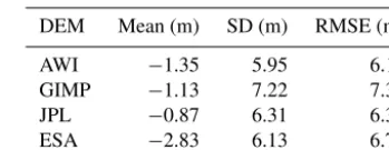
com-Table 3.Validation of four different DEMs compared to IceBridge ATM elevation data. Based on the weighted (number of samples) average of the four different ATM campaigns from 2011 to 2014. Elevation values at each ATM location were estimated by bilinear interpolation for each DEM product.
DEM Mean (m) SD (m) RMSE (m)
AWI −1.35 5.95 6.12 GIMP −1.13 7.22 7.32 JPL −0.87 6.31 6.39 ESA −2.83 6.13 6.76
parison are summarized in Table 3 as the weighted average of the different campaigns. The values from each individual campaign can be found in the Supplement.
Analyzing the overall RMSE we find that the AWI pro-duces the lowest RMSE, followed by JPL, ESA, and GIMP, due to AWI’s lower standard deviation. However, the best accuracy is obtained by the JPL DEM, which shows the lowest elevation bias of all DEMs. The ESA-derived DEM shows a slightly better standard deviation than the JPL DEM, which can probably be explained by higher data density in the marginal areas for the ESA data. The difference in den-sity is probably due to the SNR rejection criterion applied in our elevation processing. The lower standard deviation in the AWI product is most likely due to the use of lower resolu-tion topography in many of the high-relief areas in the 1 km elevation model, producing a smoother estimate of the sur-face. The GIMP data set showed higher degrees of impulse noise than the other products, explaining the higher observed standard deviation. This impulse noise is attributed to the lo-cal elevation change rate, which was not accounted for in the creation of the DEM (Howat et al., 2014). Overall we find that the JPL DEM provides a suitable compromise be-tween resolving local detail and minimizing bias. Further-more, modification to the SNR filtering criteria will likely lead to additional improvements in the DEM.
To determine the effect of retracking on the accuracy and precision of the measured surface heights from CryoSat-2 several tests were performed over different parts of Green-land for both modes. Following the approach of Davis (1997) the accuracy (mean) and precision (standard deviation) were computed as a function of leading-edge threshold (in per-cent). This computation was performed using a standard leading-edge threshold retracker, referred to from now on as LTH, for both the LRM and SIN data independently. The val-idation was performed in the same manner as described in Sect. 5, where ATM elevations from 2013 were used as the surface reference.
dif-ferent thresholds. This produced approximately 1000 com-parison locations, which were used to calculate statistics. The same procedure was performed over Jakobshavn Isbræ, using the same time span, to calculate statistics for the SIN mode, providing roughly 2500 comparison locations.
The results of this analysis, summarized in Fig. 2, show that for the LRM data the precision (as a function of thresh-old) follows the same behavior as observed by Davis (1997), with a decrease of precision following increasing retracking threshold. However, the most notable finding was the ob-served inverse relationship in precision for the SIN mode data compared to the LRM data. For the LTH algorithm in the SIN mode, we observe a clear increase in precision as the retracking threshold increases, seen in Fig. 2, stabilizing around 30–40 %.
Analyzing the accuracy derived from the different thresh-olds, a clear difference in apparent penetration depth of the radar signal can be observed for the two modes. For the SIN mode, below 40 % a positive bias is observed, indicating that retracker produces elevations larger than the corresponding airborne-measured heights. For thresholds larger than 40 % surface penetration of the signal is observed, which is in gen-eral closer to the surface compared to the LRM data. We at-tribute this to differences in the near-surface density structure covered by the two modes.
In general we conclude that for the LRM data, applying low retracking thresholds (0–30 %) reduces the magnitude of the apparent surface penetration bias and provides higher precision compared to higher thresholds. Therefore, a thresh-old of∼20 % of the leading edge is suggested for retracking surface elevations for the LRM data, which was also pre-viously suggested by Davis (1997) and Helm et al. (2014). However, for the SIN mode a threshold below 40 % is not recommended, as this produces a clear positive elevation bias and poor precision, as seen in Fig. 2. Analyzing the differ-ence between the LTH and the adaptive LMG algorithm, used in the SIN mode, we find that the LMG algorithm produces superior results in precision compared to the standard LTH algorithm. Comparing the adaptive solution from LMG to the optimum threshold (40 %) found by the LTH algorithm, we find a comparable magnitude of the elevation bias and a 32 % improvement in precision with an overall 27 % reduction in RMSE using the LMG retracker. From this comparison be-tween the two retracker algorithms we recommend the use of the adaptive threshold approach (LMG), as it produces an el-evation repeatability that exceeds that of the standard thresh-old retracker (LTH) and provides a low penetration bias.
A case study was also performed to determine the different effects of the processing steps on the quality of the retrieved elevations. For this purpose the Barnes Ice Cap, on Baffin Island in the Canadian Arctic, was chosen due to its small size, excellent validation coverage, and because it consists mostly of super-imposed ice (reducing radar signal penetra-tion). The ice cap saw a major IceBridge ATM campaign in 2011 providing a large number of flight tracks (spanning in
both north–south and east–west directions) suitable for val-idating CryoSat-2 data. The result of this case study, which is detailed in the supplementary material (i.e., Table S1 in Supplement) shows that the filtering of the differential phase has the highest impact on the overall accuracy of the observa-tion, reducing the RMSE by 12 %, followed by the ambiguity correction. This shows the importance of these steps, as they can have important implications for the overall quality of the retrieved elevations. This is especially true in high-relief ar-eas where small changes in the look angle, or an introduced phase ambiguity, can produce large elevation errors ranging from 0 to 100 m in elevation (Brenner et al., 1983).
6 Error analysis
To compute volume change errors for the two methods we divide the error budget into two main components: (1) the observational standard error (εobs)and (2) the interpolation standard error (εint).
The observational error budget is estimated using the root-mean-square error (RMSE) of the difference between CryoSat-2 and airborne elevation change differences, as de-scribed in Sect. 5. The RMSE is estimated separately from the two different modes, with the total volume change er-ror (εvol) being computed as the root sum of squares (RSS) of the standard elevation change error of the two modes and their corresponding area, according to
εvol= q
(εlrmAlrm)2+(εsinAsin)2, (12) whereAlrmandAsinare the areas covered by each mode. The
εlrm andεsinare the standard elevation change errors of the LRM and SIN data computed from the airborne validation data sets.
The observational elevation-change error is estimated from the residual elevation change differences in Table 2 for the two methods. The RMSE from the LRM/SIN data errors are computed using Gaussian error propagation producing an observational elevation change error (σobs). For the surface-fit and the crossover method the interpolation error is esti-mated as the RMS of the LSC uncertainty grid, defined as (σint). The final elevation change error is then estimated by combing the two error sources using RSS according to
εmode=εdh/dt = q
(εobs)2+(εint)2
= s
σ obs √
Nρ
2 +
σ int √
Nρ
2
. (13)
Here,Nρis the number of uncorrelated grid cells estimated from empirical semi-variogram analysis of the CryoSat-2 and airborne elevation change differences, and estimated ac-cording to
Nρ=Amode
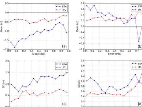
Figure 1.Validation of surface elevations (2012)(a, c)and surface elevation changes (2011–2014)(b, d)compared to IceBridge ATM, as a function of surface slope. The accuracy of the measurement is defined as the mean value (Mean) of the CryoSat-2-ATM residuals and the precision as the standard deviation (SD).
where Amode is the total area covered by each CryoSat-2 mode and the correlation lengthρmodeof 75 and 100 km for the LRM and SIN data, respectively.
7 Results
7.1 Surface elevations compared to ATM
The measured surface elevations from the two CryoSat-2 products (JPL vs. ESA) showed large differences in both accuracy and precision of the elevation measurements, as seen in Table 1. The average accuracy and precision for the LRM data from the two products of 0.00±0.43 m and −1.06±0.89 m for the JPL and ESA products, respectively. This corresponds to an average reduction in RMSE of 68 % for the JPL product compared to the ESA LRM L2 data. Furthermore, our product shows a lower residual slope er-ror (seen in Fig. 1c below ∼0.5◦) indicating a lower sensi-tivity to the degradation of performance as the surface slope increases.
Surface elevations generated from the SIN mode showed the same type of improvement as for the LRM data. Here, an average accuracy and precision were found to be −0.52±0.58 m and −0.90±1.05 m for the JPL and ESA SIN elevation products, respectively. This further corre-sponds to a reduction in the average RMSE of 27 % for the JPL product compared to the ESA product. For the SIN mode the JPL processing produces a slightly lower residual slope error, compared to the ESA processor (seen in Fig. 1c above ∼0.5◦)
Figure 2.Comparison of accuracy(a)and precision(b)as a func-tion of the retracking threshold for the leading edge threshold re-tracker (LTH, dots) applied to the LRM (red) and SIN (blue) data and the leading edge maximum gradient retracker (LMG, dashed grey line) applied to the SIN data over Jakobshavn Isbræ and the region around the NEEM camp (77◦270N, 51◦3.60W) for the LRM data. The accuracy (mean) and the precision (standard deviation) has been determined for each threshold level using near-coincident ATM elevation, within a search radius of 50 m. The statistics were estimated using CryoSat-2 data from March to May 2013 and com-pared to ATM data from April 2013.
Larger improvements can be observed if separating the RMSE into its mean and standard deviation, corresponding to the accuracy and precision of the measurements. Using these definitions the analysis found that there is a 45 and 52 % increase in precision for the SIN and LRM data, re-spectively, compared to the ESA L2 product, and a 42 and 99 % improvement in accuracy for the respective modes.
The implementation of the LMG SIN retracking algorithm was found to reduce noise in the retrieved surface eleva-tions compared to conventional threshold retracking. Though roughly comparable in accuracy, the LMG shows overall higher precision over all comparable leading edge thresholds. The adaptive nature of the algorithm provides improved esti-mates of surface elevation and a good trade-off between ac-curacy and precision.
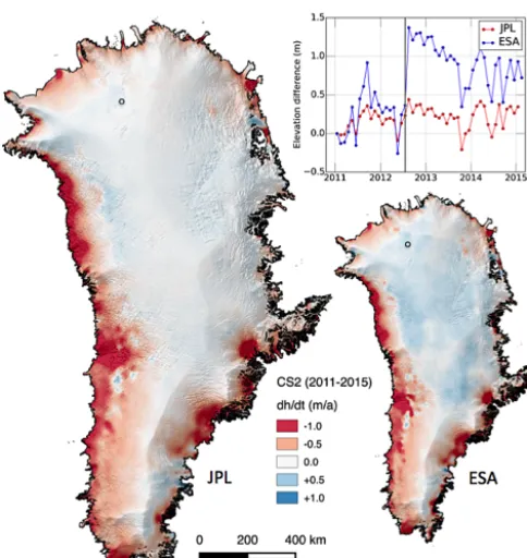
Figure 3.2011–2015 elevation changes estimated from the surface-fit method for the different L2 products. The time series depicted in the figure were extracted at the NEEM camp (77◦270N, 51◦3.60W), indicated by the black circle in both maps. The time series show the effect of the 2012 melt event, indicated by the grey vertical line, on the retrieved surface elevations. The JPL product produced a to-tal volume change of−289±20 km3a−1while the estimated total volume change of the ESA product was−224±38 km3a−1. This corresponds to −29 vs. 38 km3a−1 (H >2000 m) and −259 vs. −262 km3a−1(H <2000 m) for the JPL and ESA products, re-spectively. Images have been smoothed with a 10 km median filter for visualization purposes. The 1×1 km ice sheets mask used in this figure was constructed from polygons obtained from Frank Paul at the University of Zurich (personal communication, 2011).
for the ESA-derived changes. This corresponds to an increase in elevation change accuracy of 56 and 12 % for the LRM and SIN data, respectively, for the JPL product compared to ESA L2 elevation changes. The estimated elevation changes for the JPL product also show an increase in precisions of 56 and 45 % for the LRM and SIN data, respectively, compared to its ESA counterpart.
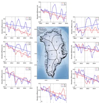
The estimated elevation changes of the Greenland Ice Sheet, excluding the peripheral glaciers, over the period of January 2011 to January 2015, show significant differences between products (JPL and ESA) in both spatial patterns and the total magnitude (Figs. 3, 4). The surface-fit and crossover methods produced on the order of∼20 and∼2.5 million us-able elevation changes, respectively, providing high spatial sampling. Due to the constraint put into the JPL processor, the ESA L2 data produced slightly more surface-fit observa-tions (∼10 %), as more surface elevations were accepted.
The ESA product produces a more positive elevation change pattern, which can be attributed to the 2012 melt event that introduced a large positive bias with a magni-tude of∼0.5 m (Nilsson et al., 2015a). Larger differences in the marginal areas for the surface-fit methods are also ob-served. The positive signal detected in the interior of the ESA surface-fit solution can also be found in the basin time series, correlating well with the timing of the summer of 2012 melt event, which can be seen in the time series in Fig. 3. These results are in agreement with earlier work demonstrating the sensitivity of the ESA retracker to the changes in the vol-ume / surface scattering ratio (Nilsson et al., 2015a).
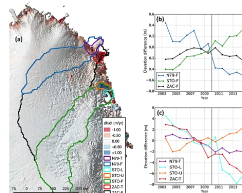
We used ICESat- and CryoSat-2-derived surface heights to generate time series over three regions in northeastern area of Greenland (Zachariæ Isstrøm, Nioghalvfjerdsfjorden and Storstrømmen glaciers) for comparison purposes. These ar-eas have recently shown large and rapid changes, which have been noted by, e.g., Khan et al. (2014). The selected areas were defined using hydrological basins derived by Lewis and Smith (2009), seen in Fig. 6, and were further divided into smaller areas around the termini to highlight performance for areas of rapid change. The ICESat and CryoSat-2 sur-face heights were then used to generate annual time series from 2003 to 2015 using Eq. (6). The estimated 12-year time series show overall comparable elevation change rates over both time periods (2003–2009 and 2010–2015), especially in the terminus areas, providing confidence that CryoSat-2 can reliably monitor changes in these areas.
Figure 4.Monthly elevation change time series for eight large drainage basins of the Greenland Ice Sheet generated from the ESA (blue) and the JPL solution (red). Time series were smoothed using a 3-month moving average for improved visualization. The grey vertical line indicates the timing of the 2012 melt event.
in amplitude is observed for all products. This is especially true for the ESA product, which increases its magnitude by a factor of 2.
Analyzing the amplitude patterns on a regional drainage basin level (Fig. 5c) we find good agreement between JPL CryoSat-2 and ICESat amplitude with ESA data producing consistently larger amplitudes. Regionally, the highest am-plitudes can be observed in southeastern Greenland in basins (3, 4, 5) and are consistent with regional precipitation pat-terns that show high total precipitation in these areas (Bales et al., 2009; Ettema et al., 2009).
The seasonal phase of the peak in amplitude of the sea-sonal cycle is shown in Fig. 5b, d and shows generally good agreement between the two data sets, providing the timing of the maximum of the accumulation signal, before the on-set of melt, to the months of June/July for both JPL and ESA CryoSat-2 data sets. The ICESat-derived seasonal phase shows a higher dependence on elevation where the maxi-mum of the accumulation signal is found in late May below 2000 m and late July/August above 2000 m in elevation. The
ICESat discrepancies from the CryoSat-2 data are found in specific basins. Disagreements between the retrieved phase of the peak amplitude from CryoSat-2 and ICESat data are due to differences in temporal sampling as discussed in more detail in Sect. 8.
7.4 Volume change
The two volume change methods produce consistent results from JPL-derived elevation changes, with a difference of around 1 km3a−1. The spread between volume change meth-ods is larger (50 km3a−1) when using ESA L2 data. The larger discrepancy is mostly related to the sensitivity of the various methods to the melt event. The surface-fit method produces the most negative number (least affected by the melt event and has the lowest estimated error) and is there-fore taken as the most reliable estimate for both the JPL and ESA solution.
Figure 5.Estimated seasonal amplitude(a, c)and phase offset(b, d)from the surface-fit method for CryoSat-2 (ESA, blue; JPL, red) compared to ICESat (ICE, black). Values are compared using a search radius of 50 m, using the closest point within this distance, and the phase offset is referenced from 1 January. The values of am-plitude and phase are then binned according to elevation using the median value within 100 m intervals.
−375±24 km3a−1. This difference can be attributed to dif-ference in processing methodology and to the different epoch of the data used by Helm et al. (2014) from January 2011 to January 2014. Using the corresponding epoch the JPL data gives a volume change estimate, based on the surface-fit method, of−353±26 km3a−1, well within the stated uncer-tainty of Helm et al. (2014).
To examine the regional behavior of volume change esti-mates of the Greenland Ice Sheet, gridded values from the two methods were divided into eight drainage basins accord-ing to Zwally et al. (2012). When analyzaccord-ing the elevation time series at the basin scale, clear differences can be ob-served in the annual and inter-annual behaviors (Fig. 4). The northern and interior basins (1, 2, 7, 8) all exhibit large dif-ferences (Table 4, 0–30 km3a−1) in the estimated volume change rates due to changes in the scattering regime result-ing from the 2012 melt event. In the majority of the southern basins (4, 5, 6, 7), located in areas with higher precipitation, both products show good agreement in both trends and sea-sonal amplitude estimated from the surface-fit method.
8 Discussion
The CryoSat-2 processing methodology presented here is found to produce accurate and precise measurements of ice sheet elevation and elevation change. The main improve-ments have been introduced in the SIN processor with the in-clusion of a novel type of land ice retracker (LMG), advanced phase filtering, and the inclusion of a phase ambiguity
correc-Table 4. Individual basin volume changes (km3a−1) for the surface-fit (SF) and crossover (XO) methods for the JPL and ESA product for the time period January 2011 to January 2015, with cor-responding error.
Basin SF – JPL XO – JPL SF – ESA XO – ESA
1 −26±8 −23±12 −9±14 −11±15 2 5±8 0±13 31±16 30±16 3 −38±9 −34±19 −46±16 −31±23 4 −36±7 −37±15 −42±12 −16±18 5 −19±4 −27±11 −19±7 −6±13 6 −72±7 −71±12 −75±13 −79±18 7 −56±7 −51±10 −41±14 −35±15 8 −48±8 −45±12 −23±15 −27±17
Total −289±20 −288±37 −224±38 −174±48
tion scheme. This processing approach decreased the RMSE in the surface height retrieval by approximately 27 % (45 and 42 % improvement in precision and accuracy). This improve-ment further propagated into the quality of the estimated el-evation changes for the SIN mode, with the same magni-tude of improvement (Table 2). The described SIN process-ing also generated surface elevations and elevation changes with lower sensitivity to the local surface slope, indicating a higher degree of accuracy in the geolocation and surface-range estimation.
The SIN processing methodology further includes a phase filtering and phase ambiguity correction scheme. Visual in-spections of a large number of tracks have shown more co-herent estimation of the surface locations in the JPL prod-uct, and the implementation of the phase-ambiguity correc-tion greatly reduced the number of track offsets. It was also noted that a relatively course DEM (∼1 km) could be used to resolve phase ambiguities. The detection and correction of phase ambiguities are relatively straightforward and rely mostly on the relative accuracy of the DEM. The implemen-tation of the phase-ambiguity correction is particularly im-portant when monitoring smaller ice caps and outlet glaciers, where frequent and large track offsets can bias the estimation of the underlying topography.
be seen that the observed negative elevation bias (Table 1) for ESA LRM (−1.0 m) fits well with the bias for the 50 % LRM data threshold value shown in Fig. 2a. This makes the al-gorithm more sensitive to annual and sub-annual changes in snowpack volume/surface scattering ratio, which can pro-duce spurious changes in elevation due to changes in the near-surface dielectric properties. This is clearly shown in patterns of ESA-product-derived elevation changes (Fig. 3) where a large elevation bias was introduced by the 2012 melt event (Nilsson et al., 2015a). The 20 % threshold is less sen-sitive to these types of changes (Tables 1, 2) and the results are in agreement with previous work that has demonstrated that the 20 % threshold best represents the mean surface in-side the footprint when exposed to a combination of surface and volume scattering (Davis, 1997).
Surface elevation changes, derived from multi-temporal radar altimetry observations, are typically corrected for their correlation to changes in the radar waveform shape. This is to reduce the effect of changes in the volume / surface scatter-ing ratio of the ice sheets’ surface (Davis, 2005; Flament and Rémy, 2012; Wingham et al., 2006b; Zwally et al., 2005). This inherently adds to the complexity of the processing and analysis, introducing new biases and error sources in the es-timated parameters. For the processing approach presented here many of the post-processing steps can be omitted or re-duced, as they are an inherent part of the improved wave-form retracking. There have been attempts to remove spuri-ous step changes in elevation resulting from sudden changes in surface-scattering characteristics (caused by the 2012 melt event) apparent in the ESA Baseline-B L2 data through post-processing strategies (Nilsson et al., 2015c; McMillan et al., 2016), but such approaches spread the bias over a longer period of time making the “jumps” less noticeable in the time series by removing the step change. However, these strate-gies introduce longer-timescale bias of equal magnitude as the scattering layer is buried by less reflective snow and low-density firn.
The result of the validation procedure shows a larger slope-dependent bias in the ESA data, both in the elevation and elevation changes (Fig. 1). This is especially true for the surface elevations, which can be seen in the figures of pre-cision and accuracy (Fig. 1a, c), where both figures show clear linear slope for the ESA surface heights. In compari-son, estimated elevations from JPL product show relatively stable statistics over the entire slope range above 0.2◦. The validation of the estimated surface elevation changes, seen in Fig. 1b and d, shows the effect of the 2012 melt event on the ESA-derived elevation changes below 0.2◦. Furthermore, the accuracy of the ESA-derived changes shows a clear negative trend as function of increased surface slope. The derived pre-cision of the surface elevation change decreases dramatically above 0.5◦, as more complex topography is measured.
The JPL CryoSat-2 processing methodology produces sea-sonal amplitudes that are in good agreement with those de-rived from ICESat data, further indicating the processors’
abilities to track real and physical changes of the ice sheet surface. The current ESA implementation produces noisier estimates of elevation change, as indicated by the larger stan-dard deviations of the residuals in the ESA solutions for the surface-fit and crossover methods. Figure 5 further shows an amplitude bias in the ESA data compared to the correspond-ing ICESat reference amplitudes. The bias is constant above the Greenland ELA, located around 2000 m in altitude, but increases linearly as elevations decrease below this. The lin-ear increase in amplitude seems to be connected to the higher and more variable precipitation in the ablation zone where changes in the variable snow cover produce changes in ap-parent surface height. This is less prominent for the JPL SIN and LRM data retrackers. The estimated seasonal phase in Fig. 5b and d shows that both JPL and ESA CryoSat-2 el-evation products can adequately resolve the seasonal max-imum of the accumulation signal. Both products provide a timing of the maximum to the month of July over the entire ice sheet, independent of elevation. Assessing the CryoSat-2-derived maximum reveals a difference between CryoSat-2 and the reference ICESat data set. This constitutes roughly a ±1-month difference depending on the elevation and the lo-cation. The cause of this difference can be attributed to the temporal sampling of the ICESat mission. During the mis-sion, due to degraded laser lifespan, data were only collected in campaign mode during the spring and winter times cor-responding to roughly 2 months of measurements for each period. When the CryoSat-2 data were resampled to coincide with the ICESat temporal sampling the same elevation and spatial pattern in the phase of the maximum seasonal ampli-tude was observed as determined from the ICESat data. No corresponding change in amplitude was observed. This was done by selecting CryoSat-2 data corresponding to the same unique months available in the total ICESat record.
The two independent methods used to estimate the vol-ume change of the Greenland Ice Sheet produce consistent volume change estimates. This was especially true for vol-ume changes derived from the JPL elevations, with a dis-crepancy of less than 1 km3a−1between methods. The two methods provided the same estimate of integrated volume change, but the use of the surface fit is recommended as it produces higher spatial sampling compared to the crossover-method and lower errors. The good agreement between the methods further indicates a strong reliability in the esti-mated volume change rates of the Greenland Ice Sheet over the 4-year period. It also shows the ability of CryoSat-2 to capture both small- and large-scale spatial patterns in the rugged topography along the coastline and in the interior of Greenland. This is especially true in the major outlet-glacier systems (e.g., Zachariæ Isstrøm, Nioghalvfjerdsfjorden, and Storstrømmen).
Zacahariæ Isstrøm, Nioghalvfjerdsfjorden, and Storstrøm-men, which all show complex and localized patterns of el-evation change. Here, Nioghalvfjerdsbrae shows very small changes in elevation during the observational time span, while Zacahariæ Isstrøm, its major neighbor, shows large negative trends in elevation change. The observed behav-ior agrees with the observations made in recent studies by Khan et al. (2014) and Mouginot et al. (2015), who document rapid retreat and drawdown of the ice-front position of the Zacahariæ Isstrøm beginning in 2012. Storstrømmen outlet glacier system also appears to show signs of rapid thinning at low elevations near the ice-front position, while a large positive signal is observed roughly 100 km upstream of the terminus. This pattern has also been observed by Joughin et al. (2010) and Thomas et al. (2009), using airborne altime-try and surface velocity mapping. Rates of elevation change from ICESat and CryoSat-2 data show good agreement in basin-scale trends (Fig. 6b, c) over the 2003–2009 and 2010– 2015 time spans.
Mass loss of the Greenland Ice Sheet was estimated for comparison purposes from the Gravity Recovery Climate Experiment (GRACE) satellite for the matching CryoSat-2 time period of 2011–2015 (Wiese et al., 2015; Watkins et al., 2015). Converting the estimated mass change to volume change, assuming no changes in firn air content over the study period and an ice density of 917 kg m−3 (assessment of changes in firn air content is out of the scope of this pa-per), gives an ice sheet wide rate of−305±38 km3a−1 (up-dated to Schlegel et al., 2016). This estimate is corrected for volume changes from peripheral glaciers that lost volume at a rate of approximately −40±27 km3a−1(Box, 2013; Fet-tweis et al., 2013; Noël et al., 2015). This estimate of periph-eral glacier change is in agreement with the estimated volume change of−41±8 km3a−1from Gardner et al. (2013). The volume rate derived from GRACE data agrees well with our estimated rate from CryoSat-2, where both results are within the 1σ uncertainty of each other and neglecting changes in firn air content over the period of study. The observed volume change rates estimated from this study are within the range of previous studies, ranging from−186 to−309 km3a−1for the time period 2003–2009, summarized by Csatho et al. (2014), using the same mass-to-volume conversion applied to the GRACE data. A more recent study by Helm et al. (2014) of−375±24 km3a−1agrees within uncertainties when dif-ferences in observation periods (2011–2014 vs. 2011–2015) are taken into account. From this comparison we find that our estimate spans both the estimate of Csatho et al. (2014) and the mass loss estimated from GRACE, while acknowledging the varied time spans of the different studies.
9 Summary and conclusion
We conclude that the use of an adaptive retracker for the SIN mode, based on the maximum gradient method, and the use
Figure 6.Northeast part of the Greenland Ice Sheet showing surface elevation change(a)from CryoSat-2 JPL solution (2011–2015), with corresponding hydrological basin outlines. The hydrological basins are separated into full basin size (b) and to the terminus areas(c).(b, c)Show a merged 12-year annual elevation time se-ries from ICESat and CryoSat-2 for each color-coded area in(a). The derived elevation time series was formed using the surface-fit method described in Sect. 3.1 onto a 500 m grid to facilitate merg-ing of the two data sets due to their difference in orbit characteris-tics. The elevation change map is overlaid onto the CryoSat-2 hill-shaded DEM based on surface heights from July 2010 to February 2015. The annual 12-year time series was created from the surface-fit method by binning the monthly values into annual values using the median of the corresponding 12 months. The gray vertical line indicates the temporal separation between the ICESat and CryoSat-2 missions.
of a 20 % threshold retracker for the LRM data provide im-proved performance to the retracker currently used for the ESA L2 elevation products. It is further important, especially for the SIN mode, to apply a leading edge discriminator to identify and track the leading edge of the waveform. The functional model currently employed in the ESA processor has, to the author’s knowledge, no such discriminator cur-rently implemented. This is important in the SIN mode, as it often contains multiple surface returns. The single-return model applied in the ESA processor will have issues fitting a waveform containing multiple surface returns resulting in retrack jitter (Helm et al., 2014).
changes with an reduction in RMSE of 55 and 40 % for the LRM and SIN data, respectively, compared to their ESA L2-derived data.
The methodology also showed less sensitivity to changes in near-surface scattering properties than equivalent ESA products. The new processing methodology showed little ef-fect of slope-induced errors, providing better performance in the marginal areas of the ice sheets. These improve-ments to the CryoSat-2 processing mitigate the need for post-processing to correct for the correlation between changes in surface elevation and changes in the waveform shape (i.e., backscatter and leading edge width etc.) that can introduce biases and add to the complexity of the processing and anal-ysis.
The presented CryoSat-2 processing methodology pro-vides a lower intrinsic error in the measured elevation, eleva-tion change, and volume change estimates, all of which will facilitate improved understanding of the geophysical process leading to changes in land ice elevation. Given the release of the ESA Baseline-C, which provides improved corrections and processing mainly for the L1B product, further improve-ments are expected in the near future.
10 Data availability
The complete DEM and elevation change grids used in this study are available upon request to the corresponding author and are provided in GeoTIFF format
The Supplement related to this article is available online at doi:10.5194/tc-10-2953-2016-supplement.
Acknowledgements. We are deeply thankful for the guidance of Laurence Gray and the support of David Burgess. We also thank Sebastian Bjerregaard Simonsen for very fruitful discussions. Furthermore, we thank Frank Paul at the University of Zurich for providing us with polygon outlines of the Greenland Ice Sheet, and the European Space Agency for providing their CryoSat-2 L1b product. We are very grateful to the editor, E. Berthier, the reviewer, L. Schröder, and an anonymous reviewer for their thoughtful and thorough comments that greatly improved the writing and content of the article. We also thank Nicole-Jeanne Schlegel and David Wiese at the Jet Propulsion Laboratory for the use of their GRACE analysis. This publication is contribution 86 of the Nordic Centre of Excellence SVALI funded by the Nordic Top-level Research Initiative. This work was supported by funding from the NASA Cryosphere program. The research was conducted at the Jet Propulsion Laboratory, California Institute of Technology, under contract with NASA.
Edited by: E. Berthier
Reviewed by: L. Schröder and one anonymous referee
References
Abulaitijiang, A., Andersen, O. B., and Stenseng, L.: Coastal sea level from inland CryoSat-2 interferometric SAR altimetry, Geo-phys. Res. Lett., 42, 1841–1847, doi:10.1002/2015GL063131, 2015.
Arthern, R., Wingham, D., and Ridout, A.: Controls on ERS al-timeter measurements over ice sheets: Footprint-scale topogra-phy, backscatter fluctuations, and the dependence of microwave penetration depth on satellite orientation, J. Geophys. Res., 106, 33471–33484, doi:10.1029/2001JD000498, 2001.
Bales, R. C., Guo, Q., Shen, D., McConnell, J. R., Du, G., Burkhart, J. F., Spikes, V. B., Hanna, E., and Cappelen, J.: Annual accumu-lation for Greenland updated using ice core data developed dur-ing 2000-2006 and analysis of daily coastal meteorological data, J. Geophys. Res., 114, D06116, doi:10.1029/2008JD011208, 2009.
Bamber, J. L.: Ice sheet altimeter processing scheme, Int. J. Remote Sens., 15, 925–938, doi:10.1080/01431169408954125, 1994. Borsa, A. A., Moholdt, G., Fricker, H. A., and Brunt, K. M.: A range
correction for ICESat and its potential impact on ice-sheet mass balance studies, The Cryosphere, 8, 345–357, doi:10.5194/tc-8-345-2014, 2014.
Bouzinac, C.: CryoSat product handbook, European Space Agency, ESA, available at: https://earth.esa.int/documents/ 10174/125272/CryoSat_Product_Handbook, last access: Octo-ber 2016, 2014.
Box, J. E.: Greenland Ice Sheet Mass Balance Reconstruction. Part II: Surface Mass Balance (1840–2010)∗, J. Climate, 26, 6974–6989, doi:10.1175/JCLI-D-12-00518.1, 2013.
Brenner, A. C., Blndschadler, R. A., Thomas, R. H., and Zwally, H. J.: Slope-induced errors in radar altimetry over continental ice sheets, J. Geophys. Res., 88, 1617, doi:10.1029/JC088iC03p01617, 1983.
Brenner, A. C., DiMarzio, J. P., and Zwally, H. J.: Precision and accuracy of satellite radar and laser altimeter data over the continental ice sheets, IEEE T. Geosci. Remote, 45, 321–331, doi:10.1109/TGRS.2006.887172, 2007.
Csatho, B. M., Schenk, A. F., van der Veen, C. J., Babo-nis, G., Duncan, K., Rezvanbehbahani, S., van den Broeke, M. R., Simonsen, S. B., Nagarajan, S., and van Angelen, J. H.: Laser altimetry reveals complex pattern of Greenland Ice Sheet dynamics, P. Natl. Acad. Sci. USA, 111, 18478–18483, doi:10.1073/pnas.1411680112, 2014.
Davis, C. H.: Surface and volume scattering retracking algorithm for ice sheet satellite altimetry, IEEE T. Geosci. Remote, 31, 811–818, doi:10.1109/36.239903, 1993.
Davis, C. H.: A robust threshold retracking algorithm for measuring ice-sheet surface elevation change from satellite radar altimeters, IEEE T. Geosci. Remote, 35, 974–979, doi:10.1109/36.602540, 1997.
Davis, C. H.: Snowfall-Driven Growth in East Antarctic Ice Sheet Mitigates Recent Sea-Level Rise, Science., 308, 1898–1901, doi:10.1126/science.1110662, 2005.
Davis, C. H. and Ferguson, A. C.: Elevation change of the antarctic ice sheet, 1995–2000, from ERS-2 satellite radar altimetry, IEEE T. Geosci. Remote, 42, 2437–2445, doi:10.1109/TGRS.2004.836789, 2004.
surface mass balance of the Greenland ice sheet revealed by high-resolution climate modeling, Geophys. Res. Lett., 36, 1–5, doi:10.1029/2009GL038110, 2009.
Fettweis, X., Franco, B., Tedesco, M., van Angelen, J. H., Lenaerts, J. T. M., van den Broeke, M. R., and Gallée, H.: Estimating the Greenland ice sheet surface mass balance contribution to fu-ture sea level rise using the regional atmospheric climate model MAR, The Cryosphere, 7, 469–489, doi:10.5194/tc-7-469-2013, 2013.
Flament, T. and Rémy, F.: Dynamic thinning of Antarctic glaciers from along-track repeat radar altimetry, J. Glaciol., 58, 830–840, doi:10.3189/2012JoG11J118, 2012.
Galin, N., Wingham, D. J., Cullen, R., Fornari, M., Smith, W. H. F., and Abdalla, S.: Calibration of the CryoSat-2 interferometer and measurement of across-track ocean slope, IEEE T. Geosci. Re-mote, 51, 57–72, doi:10.1109/TGRS.2012.2200298, 2013. Gardner, A. S., Moholdt, G., Cogley, J. G., Wouters, B., Arendt,
A. A., Wahr, J., Berthier, E., Hock, R., Pfeffer, W. T., Kaser, G., Ligtenberg, S. R. M., Bolch, T., Sharp, M. J., Hagen, J. O., van den Broeke, M. R., and Paul, F.: A reconciled estimate of glacier contributions to sea level rise: 2003 to 2009, Science, 340, 852–857, doi:10.1126/science.1234532, 2013.
Gray, L., Burgess, D., Copland, L., Cullen, R., Galin, N., Hawley, R., and Helm, V.: Interferometric swath processing of Cryosat data for glacial ice topography, The Cryosphere, 7, 1857–1867, doi:10.5194/tc-7-1857-2013, 2013.
Gray, L., Burgess, D., Copland, L., Demuth, M. N., Dunse, T., Lan-gley, K., and Schuler, T. V.: CryoSat-2 delivers monthly and inter-annual surface elevation change for Arctic ice caps, The Cryosphere, 9, 1895–1913, doi:10.5194/tc-9-1895-2015, 2015. Helm, V., Humbert, A., and Miller, H.: Elevation and elevation
change of Greenland and Antarctica derived from CryoSat-2, The Cryosphere, 8, 1539–1559, doi:10.5194/tc-8-1539-2014, 2014.
Herzfeld, U. C.: Least-squares collocation, geophysical inverse the-ory and geostatistics: a bird’s eye view, Geophys. J. Int., 111, 237–249, doi:10.1111/j.1365-246X.1992.tb00573.x, 1992. Howat, I. M., Smith, B. E., Joughin, I., and Scambos, T. A.: Rates
of southeast Greenland ice volume loss from combined ICE-Sat and ASTER observations, Geophys. Res. Lett., 35, 1–5, doi:10.1029/2008GL034496, 2008.
Howat, I. M., Negrete, A., and Smith, B. E.: The Greenland Ice Mapping Project (GIMP) land classification and surface eleva-tion data sets, The Cryosphere, 8, 1509–1518, doi:10.5194/tc-8-1509-2014, 2014.
Joughin, I., Smith, B. E., Howat, I. M., Scambos, T., and Moon, T.: Greenland flow variability from ice-sheet-wide velocity mapping, J. Glaciol., 56, 415–430, doi:10.3189/002214310792447734, 2010.
Khan, S. A., Kjaer, K. H., Bevis, M., Bamber, J. L., Wahr, J., Kjeldsen, K. K., Bjork, A. A., Korsgaard, N. J., Stearns, L. A., van den Broeke, M. R., Liu, L., Larsen, N. K., and Muresan, I. S.: Sustained mass loss of the northeast Greenland ice sheet triggered by regional warming, Nature Climate Change, 4, 292– 299, doi:10.1038/nclimate2161, 2014.
Khvorostovsky, K. S.: Merging and Analysis of Elevation Time Series Over Greenland Ice Sheet From Satellite Radar Altimetry, IEEE T. Geosci. Remote, 50, 23–36, doi:10.1109/TGRS.2011.2160071, 2012.
Krabill, W. B.: IceBridge ATM L4 Surface Elevation Rate of Change, [indicate subset used]. Boulder, Colorado USA: NASA DAAC at the National Snow and Ice Data Center, doi:10.5067/BCW6CI3TXOCY, 2014, updated 2016.
Krabill, W. B., Abdalati, W., Frederick, E. B., Manizade, S. S., Mar-tin, C. F., Sonntag, J. G., Swift, R. N., Thomas, R. H., and Yun-gel, J. G.: Airborne laser altimetry mapping of the Greenland ice sheet?: application to mass balance assessment, J. Geodyn., 34, 357–376, doi:10.1016/s0264-3707(02)00048-0, 2002.
Lacroix, P., Dechambre, M., Legrésy, B., Blarel, F., and Rémy, F.: On the use of the dual-frequency ENVISAT altimeter to deter-mine snowpack properties of the Antarctic ice sheet, Remote Sens. Environ., 112, 1712–1729, doi:10.1016/j.rse.2007.08.022, 2008.
Lewis, S. M. and Smith, L. C.: Hydrologic drainage of the Greenland Ice Sheet, Hydrol. Process., 23, 2004–2011, doi:10.1002/hyp.7343, 2009.
McMillan, M., Leeson, A., Shepherd, A., Briggs, K., Armitage, T. W. K., Hogg, A., Kuipers Munneke, P., van den Broeke, M., Noël, B., van de Berg, W. J., Ligtenberg, S., Horwath, M., Groh, A., Muir, A., and Gilbert, L.: A high-resolution record of Greenland mass balance, Geophys. Res. Lett., 43, 7002–7010, doi:10.1002/2016GL069666, 2016.
Moholdt, G., Nuth, C., Hagen, J. O., and Kohler, J.: Recent elevation changes of Svalbard glaciers derived from ICE-Sat laser altimetry, Remote Sens. Environ., 114, 2756–2767, doi:10.1016/j.rse.2010.06.008, 2010.
Mouginot, J., Rignot, E., Scheuchl, B., Fenty, I., Khazendar, A., Morlighem, M., Buzzi, A., and Paden, J.: Fast retreat of Zachariae Isstrom, northeast Greenland, Science, 350, 1357– 1361, doi:10.1126/science.aac7111, 2015.
Nilsson, J., Vallelonga, P., Simonsen, S. B., Sørensen, L. S., Fors-berg, R., Dahl-Jensen, D., Hirabayashi, M., Goto-Azuma, K., Hvidberg, C. S., Kjaer, H. A., and Satow, K.: Greenland 2012 melt event effects on CryoSat-2 radar altimetry, Geophys. Res. Lett., 42, 3919–3926, doi:10.1002/2015GL063296, 2015a. Nilsson, J., Sandberg Sørensen, L., Barletta, V. R., and Forsberg,
R.: Mass changes in Arctic ice caps and glaciers: implications of regionalizing elevation changes, The Cryosphere, 9, 139–150, doi:10.5194/tc-9-139-2015, 2015b.
Nilsson, J., Forsberg, R., and Sandberg Sørensen, L.: Cryosphere Monitoring from Satellites and Aircrafts, PhD thesis, Technical University of Denmark, Kgs. Lyngby, 2015c.
Noël, B., van de Berg, W. J., van Meijgaard, E., Kuipers Munneke, P., van de Wal, R. S. W., and van den Broeke, M. R.: Evalua-tion of the updated regional climate model RACMO2.3: summer snowfall impact on the Greenland Ice Sheet, The Cryosphere, 9, 1831–1844, doi:10.5194/tc-9-1831-2015, 2015.
Poinar, K., Joughin, I., Das, S. B., Behn, M. D., Lenaerts, J. T. M., and van den Broeke, M. R.: Limits to future ex-pansion of surface-melt-enhanced ice flow into the interior of western Greenland, Geophys. Res. Lett., 42, 1800–1807, doi:10.1002/2015GL063192, 2015.
Qi, W. and Braun, A.: Accelerated elevation change of Greenland’s Jakobshavn glacier observed by ICESat and IceBridge, IEEE Geosci. Remote S., 10, 1133–1137, doi:10.1109/LGRS.2012.2231954, 2013.