S
PRITE: Generalizing Topic Models with Structured Priors
Michael J. Paul and Mark Dredze Department of Computer Science
Human Language Technology Center of Excellence Johns Hopkins University, Baltimore, MD 21218
[email protected],[email protected]
Abstract
We introduce SPRITE, a family of topic
models that incorporates structure into model priors as a function of underlying components. The structured priors can be constrained to model topic hierarchies, factorizations, correlations, and
supervi-sion, allowing SPRITE to be tailored to
particular settings. We demonstrate this
flexibility by constructing a SPRITE-based
model to jointly infer topic hierarchies and author perspective, which we apply to cor-pora of political debates and online re-views. We show that the model learns in-tuitive topics, outperforming several other topic models at predictive tasks.
1 Introduction
Topic models can be a powerful aid for analyzing large collections of text by uncovering latent in-terpretable structures without manual supervision. Yet people often have expectations about topics in a given corpus and how they should be structured for a particular task. It is crucial for the user expe-rience that topics meet these expectations (Mimno et al., 2011; Talley et al., 2011) yet black box topic models provide no control over the desired output.
This paper presents SPRITE, a family of topic
models that provide a flexible framework for en-coding preferences as priors for how topics should
be structured. SPRITEcan incorporate many types
of structure that have been considered in prior work, including hierarchies (Blei et al., 2003a; Mimno et al., 2007), factorizations (Paul and Dredze, 2012; Eisenstein et al., 2011), sparsity (Wang and Blei, 2009; Balasubramanyan and Co-hen, 2013), correlations between topics (Blei and Lafferty, 2007; Li and McCallum, 2006), pref-erences over word choices (Andrzejewski et al., 2009; Paul and Dredze, 2013), and associations
between topics and document attributes (Ramage et al., 2009; Mimno and McCallum, 2008).
SPRITE builds on a standard topic model,
adding structure to thepriors over the model
pa-rameters. The priors are given by log-linear
func-tions of underlyingcomponents(§2), which
pro-vide additional latent structure that we will show can enrich the model in many ways. By apply-ing particular constraints and priors to the compo-nent hyperparameters, a variety of structures can be induced such as hierarchies and factorizations
(§3), and we will show that this framework
cap-tures many existing topic models (§4).
After describing the general form of the model,
we show how SPRITE can be tailored to
partic-ular settings by describing a specific model for the applied task of jointly inferring topic
hierar-chies and perspective (§6). We experiment with
this topic+perspective model on sets of political
debates and online reviews (§7), and demonstrate
that SPRITElearns desired structures while
outper-forming many baselines at predictive tasks.
2 Topic Modeling with Structured Priors
Our model family generalizes latent Dirichlet al-location (LDA) (Blei et al., 2003b). Under LDA,
there are K topics, where a topic is a
categor-ical distribution overV words parameterized by
φk. Each document has a categorical distribution
over topics, parameterized byθmfor themth
doc-ument. Each observed word in a document is
gen-erated by drawing a topiczfromθm, then drawing
the word fromφz. θ andφ have priors given by
Dirichlet distributions.
Our generalization adds structure to the gener-ation of the Dirichlet parameters. The priors for these parameters are modeled as log-linear
com-binations of underlyingcomponents. Components
are real-valued vectors of length equal to the
vo-cabulary size V (for priors over word
distribu-tions) or length equal to the number of topicsK
(for priors over topic distributions).
For example, we might assume that topics about sports like baseball and football share a common prior – given by a component – with general words about sports. A fine-grained topic about steroid use in sports might be created by combining com-ponents about broader topics like sports, medicine, and crime. By modeling the priors as combina-tions of components that are shared across all top-ics, we can learn interesting connections between topics, where components provide an additional latent layer for corpus understanding.
As we’ll show in the next section, by imposing certain requirements on which components feed into which topics (or documents), we can induce a variety of model structures. For example, if we want to model a topic hierarchy, we require that each topic depend on exactly one parent compo-nent. If we want to jointly model topic and
ide-ology in a corpus of political documents (§6), we
make topic priors a combination of one component from each of two groups: a topical component and an ideological component, resulting in ideology-specific topics like “conservative economics”.
Components construct priors as follows. For the topic-specific word distributionsφ, there areC(φ)
topic components. The kth topic’s prior overφk
is a weighted combination (with coefficient vector
βk) of theC(φ)components (where componentcis
denotedωc). For the document-specific topic
dis-tributionsθ, there areC(θ)document components.
Themth document’s prior overθmis a weighted
combination (coefficientsαm) of theC(θ)
compo-nents (where componentcis denotedδc).
Once conditioned on these priors, the model is identical to LDA. The generative story is de-scribed in Figure 1. We call this family of models
SPRITE: StructuredPRIorTopic modEls.
To illustrate the role that components can play, consider an example in which we are modeling re-search topics in a corpus of NLP abstracts (as we
do in§7.3). Consider three speech-related topics:
signal processing, automatic speech recognition, and dialog systems. Conceptualized as a hierar-chy, these topics might belong to a higher level
category of spoken language processing. SPRITE
allows the relationship between these three topics to be defined in two ways. One, we can model that these topics will all have words in common. This is handled by the topic components – these three topics could all draw from a common “spoken
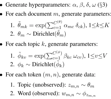
lan-• Generate hyperparameters:α,β,δ,ω(§3)
• For each documentm, generate parameters:
1. θmk˜ = exp(PC(θ)
c=1 αmcδck), 1≤k≤K
2. θm∼Dirichlet(˜θm)
• For each topick, generate parameters:
1. φ˜kv= exp(PC(φ)
c=1 βkcωcv), 1≤v≤V
2. φk∼Dirichlet( ˜φk)
• For each token(m, n), generate data:
1. Topic (unobserved):zm,n∼θm
2. Word (observed):wm,n∼φzm,n
Figure 1: The generative story of SPRITE. The difference from latent Dirichlet allocation (Blei et al., 2003b) is the gen-eration of the Dirichlet parameters.
guage” topic component, with high-weight words
such as speech and spoken, which informs the
prior of all three topics. Second, we can model that these topics are likely to occur together in docu-ments. For example, articles about dialog systems are likely to discuss automatic speech recognition as a subroutine. This is handled by the document components – there could be a “spoken language” document component that gives high weight to all three topics, so that if a document draw its prior from this component, then it is more likely to give probability to these topics together.
The next section will describe how particular priors over the coefficients can induce various structures such as hierarchies and factorizations, and components and coefficients can also be pro-vided as input to incorporate supervision and prior knowledge. The general prior structure used in SPRITE can be used to represent a wide array of
existing topic models, outlined in Section 4.
3 Topic Structures
By changing the particular configuration of the
hy-perparameters – the component coefficients (αand
β) and the component weights (δandω) – we
ob-tain a diverse range of model structures and behav-iors. We now describe possible structures and the corresponding priors.
3.1 Component Structures
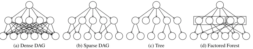
[image:2.612.321.510.38.207.2](a) Dense DAG (b) Sparse DAG (c) Tree (d) Factored Forest Figure 2: Example graph structures describing possible relations between components (middle row) and topics or documents (bottom row). Edges correspond to non-zero values forαorβ(the component coefficients defining priors over the document
and topic distributions). The root node is a shared prior over the component weights (with other possibilities discussed in§3.3).
3.1.1 Directed Acyclic Graph
The general SPRITEmodel can be thought of as a
dense directed acyclic graph (DAG), where every document or topic is connected to every
compo-nent with some weightα or β. When many of
theαorβcoefficients are zero, the DAG becomes
sparse. A sparse DAG has an intuitive interpre-tation: each document or topic depends on some subset of components.
The default prior over coefficients that we use in this study is a 0-mean Gaussian distribution, which encourages the weights to be small. We note that to induce a sparse graph, one could use
a 0-mean Laplace distribution as the prior overα
and β, which prefers parameters such that some
components are zero. 3.1.2 Tree
When each document or topic has exactly one par-ent (one nonzero coefficipar-ent) we obtain a two-level tree structure. This structure naturally arises in topic hierarchies, for example, where fine-grained topics are children of coarse-grained topics.
To create an (unweighted) tree, we require
αmc ∈ {0,1}and Pcαmc = 1 for each
docu-mentm. Similarly,βkc ∈ {0,1}andPcβkc= 1
for each topick. In this setting, αmand βk are
indicator vectors which select a single component.
In this study, rather than strictly requiringαm
andβk to be binary-valued indicator vectors, we
create a relaxation that allows for easier parameter
estimation. We letαmandβk to real-valued
vari-ables in a simplex, but place a prior over their val-ues to encourage sparse valval-ues, favoring vectors with a single component near 1 and others near 0. This is achieved using a Dirichlet(ρ <1)
distribu-tion as the prior overαand β, which has higher
density near the boundaries of the simplex.1
1This generalizes the technique used in Paul and Dredze
(2012), who approximated binary variables with real-valued variables in(0,1), by using a “U-shaped” Beta(ρ <1)
distri-For a weighted tree,αandβcould be a product
of two variables: an “integer-like” indicator vec-tor with sparse Dirichlet prior as suggested above, combined with a real-valued weight (e.g., with a Gaussian prior). We take this approach in our model of topic and perspective (§6).
3.1.3 Factored Forest
By using structured sparsity over the DAG, we can obtain a structure where components are grouped
into G factors, and each document or topic has
one parent from each group. Figure 2(d) illus-trates this: the left three components belong to one group, the right two belong to another, and each bottom node has exactly one parent from each. This is a DAG that we call a “factored forest” be-cause the subgraphs associated with each group in isolation are trees. This structure arises in “multi-dimensional” models like SAGE (Eisenstein et al., 2011) and Factorial LDA (Paul and Dredze, 2012), which allow tokens to be associated with multiple variables (e.g. a topic along with a variable denot-ing positive or negative sentiment). This allows word distributions to depend on both factors.
The “exactly one parent” indicator constraint is the same as in the tree structure but enforces a tree only within each group. This can therefore be (softly) modeled using a sparse Dirichlet prior as described in the previous subsection. In this case, the subsets of components belonging to each fac-tor have separate sparse Dirichlet priors. Using the example from Figure 2(d), the first three com-ponent indicators would come from one Dirichlet, while the latter two component indicators would come from a second.
3.2 Tying Topic and Document Components A desirable property for many situations is for the topic and document components to correspond to
each other. For example, if we think of the com-ponents as coarse-grained topics in a hierarchy,
then the coefficientsβenforce that topic word
dis-tributions share a prior defined by their parentω
component, while the coefficients α represent a
document’s proportions of coarse-grained topics, which effects the document’s prior over child
top-ics (through theδvectors). Consider the example
with spoken language topics in§2: these three
top-ics (signal processing, speech recognition, and
di-alog systems) area priorilikely both to share the
same words and to occur together in documents. By tying these together, we ensure that the pat-terns are consistent across the two types of com-ponents, and the patterns from both types can re-inforce each other during inference.
In this case, the number of topic components is the same as the number of document
compo-nents (C(φ) = C(θ)), and the coefficients (β
cz)
of the topic components should correlate with the
weights of the document components (δzc). The
approach we take (§6) is to define δ and β as a
product of two variables (suggested in§3.1.2): a
binary mask variable (with sparse Dirichlet prior),
which we let be identical for bothδ andβ, and a
real-valued positive weight.
3.3 Deep Components
As for priors over the component weightsδ and
ω, we assume they are generated from a 0-mean
Gaussian. While not experimented with in this study, it is also possible to allow the components themselves to have rich priors which are functions of higher level components. For example, rather than assuming a mean of zero, the mean could be a weighted combination of higher level weight vec-tors. This approach was used by Paul and Dredze
(2013) in Factorial LDA, in which eachω
compo-nent had its own Gaussian prior provided as input to guide the parameters.
4 Special Cases and Extensions
We now describe several existing Dirichlet prior topic models and show how they are special cases of SPRITE. Table 1 summarizes these models and
their relation to SPRITE. In almost every case, we
also describe how the SPRITE representation of
the model offers improvements over the original model or can lead to novel extensions.
Model Sec. Document priors Topic priors LDA 4.1 Single component Single component SCTM 4.2 Single component Sparse binaryβ
SAGE 4.3 Single component Sparseω
FLDA 4.3 Binaryδis transpose ofβ Factored binaryβ
PAM 4.4 αare supertopic weights Single component DMR 4.5 αare feature values Single component
Table 1: Topic models with Dirichlet priors that are gen-eralized by SPRITE. The description of each model can be found in the noted section number. PAM is not equivalent, but captures very similar behavior. The described component formulations of SCTM and SAGE are equivalent, but these differ from SPRITEin that the components directly define the
parameters, rather than priors over the parameters.
4.1 Latent Dirichlet Allocation
In LDA (Blei et al., 2003b), all θ vectors are
drawn from the same prior, as are all φ vectors.
This is a basic instance of our model with only one component at the topic and document levels,
C(θ)=C(φ)= 1, with coefficientsα=β= 1.
4.2 Shared Components Topic Models Shared components topic models (SCTM) (Gorm-ley et al., 2010) define topics as products of “com-ponents”, where components are word
distribu-tions. To use the notation of our paper, thekth
topic’s word distribution in SCTM is
parameter-ized byφkv ∝ Qcω
βkc
cv , where the ωvectors are
word distributions (rather than vectors inRV), and
theβkc ∈ {0,1}variables are indicators denoting
whether componentcis in topick.
This is closely related to SPRITE, where
top-ics also depend on products of underlying com-ponents. A major difference is that in SCTM, the topic-specific word distributions are exactly defined as a product of components, whereas in SPRITE, it is only the prior that is a product of
components.2 Another difference is that SCTM
has an unweighted product of components (βis
bi-nary), whereas SPRITEallows for weighted
prod-ucts. The log-linear parameterization leads to sim-pler optimization procedures than the product pa-rameterization. Finally, the components in SCTM only apply to the word distributions, and not the topic distributions in documents.
4.3 Factored Topic Models
Factored topic models combine multiple aspects of the text to generate the document (instead of just topics). One such topic model is Factorial LDA (FLDA) (Paul and Dredze, 2012). In FLDA,
2The posterior becomes concentrated around the prior
when the Dirichlet variance is low, in which case SPRITE
[image:4.612.318.519.43.101.2]“topics” are actually tuples of potentially multiple variables, such as aspect and sentiment in online reviews (Paul et al., 2013). Each document
distri-butionθm is a distribution over pairs (or
higher-dimensional tuples if there are more than two
fac-tors), and each pair (j, k) has a word
distribu-tion φ(j,k). FLDA uses a similar log-linear
pa-rameterization of the Dirichlet priors as SPRITE.
Using our notation, the Dirichlet(φ˜(j,k)) prior for φ(j,k)is defined asφ˜(j,k),v=exp(ωjv+ωkv), where
ωj is a weight vector over the vocabulary for the
jth component of the first factor, andωk encodes
the weights for thekth component of the second
factor. (Some bias terms are omitted for
sim-plicity.) The prior over θm has a similar form:
˜
θm,(j,k)=exp(αmj +αmk), where αmj is
docu-mentm’s preference for componentj of the first
factor (and likewise forkof the second).
This corresponds to an instantiation of SPRITE
using an unweighted factored forest (§3.1.3),
whereβzc =δcz(§3.2, recall thatδare document
components while β are the topic coefficients).
Each subtopicz (which is a pair of variables in
the two-factor model) has one parent component
from each factor, indicated byβzwhich is
binary-valued. At the document level in the two-factor
example,δjis an indicator vector with values of 1
for all pairs withjas the first component, and thus
the coefficientαmj controls the prior for all such
pairs of the form(j,·), and likewise δk indicates
pairs withkas the second component, controlling
the prior over(·, k).
The SPRITErepresentation offers a benefit over
the original FLDA model. FLDA assumes that the entire Cartesian product of the different factors is
represented in the model (e.g.φparameters for
ev-ery possible tuple), which leads to issues with effi-ciency and overparameterization with higher
num-bers of factors. With SPRITE, we can simply fix
the number of “topics” to a number smaller than the size of the Cartesian product, and the model
will learn which subset of tuples are included,
through the values ofβandδ.
Finally, another existing model family that al-lows for topic factorization is the sparse additive generative model (SAGE) (Eisenstein et al., 2011). SAGE uses a log-linear parameterization to define word distributions. SAGE is a general family of models that need not be factored, but is presented as an efficient solution for including multiple fac-tors, such as topic and geography or topic and
au-thor ideology. Like SCTM,φis exactly defined as
a product ofωweights, rather than our approach
of using the product to define a prior overφ.
4.4 Topic Hierarchies and Correlations While the two previous subsections primarily fo-cused on word distributions (with FLDA being an
exception that focused on both), SPRITE’s priors
over topic distributions also have useful
charac-teristics. The component-specific δ vectors can
be interpreted as common topic distribution pat-terns, where each component is likely to give high weight to groups of topics that tend to occur
to-gether. Each document’sαweights encode which
of the topic groups are present in that document. Similar properties are captured by the Pachinko allocation model (PAM) (Li and McCallum, 2006). Under PAM, each document has a
distri-bution over supertopics. Each supertopic is
as-sociated with a Dirichlet prior oversubtopic
dis-tributions, where subtopics are the low level
top-ics that are associated with word parameters φ.
Documents also have supertopic-specific distribu-tions over subtopics (drawn from each supertopic-specific Dirichlet prior). Each topic in a document is drawn by first drawing a supertopic from the document’s distribution, then drawing a subtopic from that supertopic’s document distribution.
While not equivalent, this is quite similar to SPRITE where document components correspond
to supertopics. Each document’sα weights can
be interpreted to be similar to a distribution over
supertopics, and eachδvector is that supertopic’s
contribution to the prior over subtopics. The prior over the document’s topic distribution is thus
af-fected by the document’s supertopic weightsα.
The SPRITE formulation naturally allows for
powerful extensions to PAM. One possibility is to include topic components for the word distri-butions, in addition to document components, and to tie togetherδczandβzc(§3.2). This models the
intuitive characteristic that subtopics belonging to
similar supertopics (encoded by δ) should come
from similar priors over their word distributions
(since they will have similarβ values). That is,
super-topic word distributions. Another extension is to form a strict tree structure, making each subtopic belong to exactly one supertopic: a true hierarchy. 4.5 Conditioning on Document Attributes SPRITEalso naturally provides the ability to
con-dition document topic distributions on features of the document, such as a user rating in a review. To do this, let the number of document compo-nents be the number of features, and the value of
αmc is themth document’s value of the cth
fea-ture. Theδvectors then influence the document’s
topic prior based on the feature values. For exam-ple, increasingαmcwill increase the prior for topic zifδcz is positive and decrease the prior ifδczis
negative. This is similar to the structure used for
PAM (§4.4), but here theαweights are fixed and
provided as input, rather than learned and inter-preted as supertopic weights. This is identical to the Dirichlet-multinomial regression (DMR) topic model (Mimno and McCallum, 2008). The DMR topic model define’s each document’s Dirichlet prior over topics as a log-linear function of the document’s feature values and regression
coeffi-cients for each topic. Thecth feature’s regression
coefficients correspond to theδcvector in SPRITE.
5 Inference and Parameter Estimation
We now discuss how to infer the posterior of the latent variableszand parametersθandφ, and find
maximuma posteriori(MAP) estimates of the
hy-perparametersα,β,δ, andω, given their hyperpri-ors. We take a Monte Carlo EM approach, using a collapsed Gibbs sampler to sample from the
pos-terior of the topic assignments z conditioned on
the hyperparameters, then optimizing the hyperpa-rameters using gradient-based optimization condi-tioned on the samples.
Given the hyperparameters, the sampling equa-tions are identical to the standard LDA sampler (Griffiths and Steyvers, 2004). The partial deriva-tive of the collapsed log likelihoodLof the corpus
with respect to each hyperparameterβkcis:
∂L ∂βkc
=∂P(β) ∂βkc
+X v
ωcvφkv˜ × (1)
Ψ(nkv+ ˜φkv)−Ψ( ˜φkv) +Ψ(Pk0φ˜k0v)−Ψ(Pk0nk 0
v + ˜φk0v)
whereφ˜kv=exp(P
c0βkc0ωc0v),nkv is the number
of times word v is assigned to topic k (in the
samples from the E-step), andΨis the digamma
function, the derivative of the log of the gamma function. The digamma terms arise from the Dirichlet-multinomial distribution, when integrat-ing out the parametersφ. P(β)is the hyperprior. For a 0-mean Gaussian hyperprior with variance
σ2, ∂P(β) ∂βkc = −
βkc
σ2. Under a Dirchlet(ρ)
hyper-prior, when we wantβ to represent an indicator
vector (§3.1.2),∂P(β)∂βkc =
ρ−1 βkc.
The partial derivatives for the other hyperpa-rameters are similar. Rather than involving a sum
over the vocabulary, ∂L
∂δck sums over documents,
while ∂L
∂ωcv and
∂L
∂αmc sum over topics.
Our inference algorithm alternates between one Gibbs iteration and one iteration of gradient as-cent, so that the parameters change gradually. For unconstrained parameters, we use the update rule: xt+1=xt +ηt∇L(xt), for some variable x and
a step sizeηt at iterationt. For parameters
con-strained to the simplex (such as whenβis a soft
indicator vector), we use exponentiated gradient ascent (Kivinen and Warmuth, 1997) with the up-date rule:xt+1i ∝xt
iexp(ηt∇iL(xt)).
5.1 Tightening the Constraints
For variables that we prefer to be binary but have softened to continuous variables using sparse Beta or Dirichlet priors, we can straightforwardly strengthen the preference to be binary by modify-ing the objective function to favor the prior more heavily. Specifically, under a Dirichlet(ρ<1) prior
we will introduce a scaling parameter τt ≥ 1
to the prior log likelihood: τtlogP(β) with
par-tial derivativeτtρβ−1
kc, which adds extra weight to
the sparse Dirichlet prior in the objective. The algorithm used in our experiments begins with
τ1 = 1and optionally increasesτover time. This
is a deterministic annealing approach, where τ
corresponds to an inverse temperature (Ueda and Nakano, 1998; Smith and Eisner, 2006).
As τ approaches infinity, the prior-annealed
MAP objective maxβP(φ|β)P(β)τ approaches maxβP(φ|β) maxβP(β). Annealing only the
prior P(β) results in maximization of this term
only, while the outermaxchooses a goodβunder
P(φ|β)as a tie-breaker among all β values that
maximize the innermax(binary-valuedβ).3
We show experimentally (§7.2.2) that annealing
the prior yields values that satisfy the constraints.
3Other modifications could be made to the objective
6 A Factored Hierarchical Model of Topic and Perspective
We will now describe a SPRITE model that
en-compasses nearly all of the structures and
exten-sions described in§3–4, followed by
experimen-tal results using this model to jointly capture topic and “perspective” in a corpus of political debates (where perspective corresponds to ideology) and a corpus of online doctor reviews (where perspec-tive corresponds to the review sentiment).
First, we will create a topic hierarchy(§4.4).
The hierarchy will model both topics and
docu-ments, whereαmis documentm’s supertopic
pro-portions,δcis thecth supertopic’s subtopic prior,
ωc is the cth supertopic’s word prior, and βk is
the weight vector that selects thekth topic’s
par-ent supertopic, which incorporates (soft) indicator vectors to encode a tree structure (§3.1.2).
We want a weighted tree; while each βk has
only one nonzero element, the nonzero element can be a value other than 1. We do this by replac-ing the sreplac-ingle coefficientβkcwith a product of two
variables:bkcβˆkc. Here,βˆkis a real-valued weight
vector, whilebkcis a binary indicator vector which
zeroes out all but one element ofβk. We do the
same with theδvectors, replacingδckwithbkcˆδck.
Thebvariables are shared across both topic and
document components, which is how we tie these
together (§3.2). We relax the binary requirement
and instead allow a positive real-valued vector whose elements sum to 1, with a Dirichlet(ρ<1)
prior to encourage sparsity (§3.1.2).
To be properly interpreted as a hierarchy, we
constrain the coefficients α and β (and by
ex-tension, δ) to be positive. To optimize these
pa-rameters in a mathematically convenient way, we
write βkc as exp(logβkc), and instead optimize
logβkc∈Rrather thanβkc∈R+.
Second, wefactorize(§4.3) our hierarchy such
that each topic depends not only on its supertopic, but also on a value indicating perspective. For ex-ample, a conservative topic about energy will ap-pear differently from a liberal topic about energy. The prior for a topic will be a log-linear combina-tion of both a supertopic (e.g. energy) and a per-spective (e.g. liberal) weight vector. The variables associated with the perspective component are de-noted with superscript(P)rather than subscriptc. To learn meaningful perspective parameters, we
include supervision in the form of document
at-tributes (§4.5). Each document includes a
pos-• bk∼Dirichlet(ρ <1)(soft indicator)
• α(P)is given as input (perspective value)
• δ(P)k =β(P)k
• φ˜kv = exp(ω(B)v +βk(P)ωv(P)+Pcbkcβˆkcωcv) • θ˜mk= exp(δ(B)k +α
(P)
m δ(P)k +Pcbkcαmcδˆck)
Figure 3: Summary of the hyperparameters in our SPRITE
-based topic and perspective model (§6).
itive or negative score denoting the perspective, which is the variableα(P)m for documentm. Since α(P) are the coefficients forδ(P), positive values
ofδk(P)indicate that topickis more likely if the
au-thor is conservative (which has a positiveαscore
in our data), and less likely if the author is liberal (which has a negative score). There is only a single perspective component, but it represents two ends of a spectrum with positive and negative weights;
β(P) andδ(P)are not constrained to be positive,
unlike the supertopics. We also setβk(P) = δk(P).
This means that topics with positiveδk(P)will also
have a positiveβcoefficient that is multiplied with
the perspective word vectorω(P).
Finally, we include “bias” component vectors
denoted ω(B) and δ(B), which act as overall
weights over the vocabulary and topics, so that the
component-specificωandδweights can be
inter-preted as deviations from the global bias weights. Figure 3 summarizes the model. This includes most of the features described above (trees, fac-tored structures, tying topic and document compo-nents, and document attributes), so we can ablate model features to measure their effect.
7 Experiments
7.1 Datasets and Experimental Setup We applied our models to two corpora:
• Debates:A set of floor debates from the 109th–
112th U.S. Congress, collected by Nguyen et al. (2013), who also applied a hierarchical topic model to this data. Each document is a tran-script of one speaker’s turn in a debate, and each document includes the first dimension of the
DW-NOMINATEscore (Lewis and Poole, 2004),
a real-valued score indicating how conservative (positive) or liberal (negative) the speaker is.
This value isα(P). We took a sample of 5,000
affilia-tion. We sampled from the most partisan speak-ers, removing scores below the median value.
• Reviews: Doctor reviews from RateMDs.com,
previously analyzed using FLDA (Paul et al., 2013; Wallace et al., 2014). The reviews con-tain ratings on a 1–5 scale for multiple aspects. We centered the ratings around the middle value 3, then took reviews that had the same sign for all aspects, and averaged the scores to produce
a value forα(P). Our corpus contains 20,000
documents (476,991 tokens; 10,158 types), bal-anced across positive/negative scores.
Unless otherwise specified, K=50 topics and
C=10 components (excluding the perspective
component) forDebates, andK=20 andC=5 for
Reviews. These values were chosen as a
qualita-tive preference, not optimized for predicqualita-tive per-formance, but we experiment with different values in§7.2.2. We set the step sizeηtaccording to
Ada-Grad (Duchi et al., 2011), where the step size is the inverse of the sum of squared historical
gradi-ents.4 We place a sparse Dirichlet(ρ=0.01) prior
on the b variables, and apply weak
regulariza-tion to all other hyperparameters via aN(0,102)
prior. These hyperparameters were chosen after only minimal tuning, and were selected because they showed stable and reasonable output qualita-tively during preliminary development.
We ran our inference algorithm for 5000
itera-tions, estimating the parametersθ andφby
aging the final 100 iterations. Our results are
aver-aged across 10 randomly initialized samplers.5
7.2 Evaluating the Topic Perspective Model 7.2.1 Analysis of Output
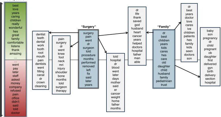
Figure 4 shows examples of topics learned from
theReviewscorpus. The figure includes the
high-est probability words in various topics as well as the highest weight words in the supertopic com-ponents and perspective component, which feed into the priors over the topic parameters. We see that one supertopic includes many words related to
surgery, such asprocedureandperformed, and has
multiple children, including a topic about dental work. Another supertopic includes words
describ-ing family members such as kids and husband.
4AdaGrad decayed too quickly for thebvariables. For
these, we used a variant suggested by Zeiler (2012) which uses an average of historical gradients rather than a sum.
5Our code and the data will be available at:
http://cs.jhu.edu/˜mpaul.
One topic has both supertopics as parents, which appears to describe surgeries that saved a family
member’s life, with top words including{saved,
life,husband,cancer}. The figure also illustrates which topics are associated more with positive or negative reviews, as indicated by the value ofδ(P).
Interpretable parameters were also learned from
the Debates corpus. Consider two topics about
energy that have polar values of δ(P). The
conservative-leaning topic is about oil and gas,
with top words including {oil, gas, companies,
prices, drilling}. The liberal-leaning topic is
about renewable energy, with top words includ-ing{energy,new,technology,future,renewable}.
Both of these topics share a common parent of an industry-related supertopic whose top words are
{industry,companies,market,price}. A nonparti-san topic under this same supertopic has top words
{credit,financial,loan,mortgage,loans}.
7.2.2 Quantitative Evaluation
We evaluated the model on two predictive tasks as well as topic quality. The first metric is perplex-ity of held-out text. The held-out set is based on tokens rather than documents: we trained on even numbered tokens and tested on odd tokens. This is a type of “document completion” evaluation (Wal-lach et al., 2009b) which measures how well the model can predict held-out tokens of a document after observing only some.
We also evaluated how well the model can
pre-dict the attribute value (DW-NOMINATE score or
user rating) of the document. We trained a linear regression model using the document topic
distri-butionsθas features. We held out half of the
docu-ments for testing and measured the mean absolute
error. When estimating document-specific SPRITE
parameters for held-out documents, we fix the fea-ture valueα(P)m = 0for that document.
These predictive experiments do not directly measure performance at many of the particular tasks that topic models are well suited for, like data exploration, summarization, and visualiza-tion. We therefore also include a metric that more directly measures the quality and interpretability
of topics. We use the topiccoherencemetric
best! love! years! caring! children! really! wonderful! hes! great! family! comfortable! listens! thank! amazing! …! …! went! pay! later! staff! asked! money! company! refused! pain! office! didn’t! said! told! doctor! surgery! pain! went! dr! surgeon! told! procedure! months! performed! removed! left! fix! said! later! years! dr! life! thank! saved! god! husband! heart! cancer! years! helped! doctors! hospital! father! man! able! told! hospital! dr! blood! went! later! days! mother! said! er! cancer! weight! home! father! months! dentist! teeth! dental! work! tooth! root! mouth! pain! dentists! went! filling! canal! dr! crown! cleaning! dr! best! children! years! kids! cares! hes! care! old! daughter! child! husband! family! pediatrician! trust! baby! son! pregnancy! dr! child! pregnant! ob! daughter! first! delivered! gyn! birth! delivery! section! hospital! dr! best! years! doctor! love! cares! ive! children! patients! hes! family! kids! seen! doctors! son! pain! surgery! dr! went! knee! foot! neck! mri! injury! shoulder! bone! months! told! surgeon! therapy! Perspective! “Surgery”! “Family”!
Figure 4: Examples of topics (gray boxes) and components (colored boxes) learned on theReviewscorpus with 20 topics and 5 components. Words with the highest and lowest values ofω(P), the perspective component, are shown on the left, reflecting positive and negative sentiment words. The words with largestωvalues in two supertopic components are also shown, with manually given labels. Arrows from components to topics indicate that the topic’s word distribution draws from that component in its prior (with non-zeroβvalue). There are also implicit arrows from the perspective component to all topics (omitted for clarity). The vertical positions of topics reflect the topic’s perspective valueδ(P). Topics centered above the middle line are more likely to occur in reviews with positive scores, while topics below the middle line are more likely in negative reviews. Note that this is a “soft” hierarchy because the tree structure is not strictly enforced, so some topics have multiple parent components. Table 3 shows how strict trees can be learned by tuning the annealing parameter.
measure the average coherence across all topics:
1 K K X k=1 M X m=2 mX−1
l=1
logDF(vkm, vkl) + 1 DF(vkl) (2)
where DF(v, w) is the document frequency of
wordsvandw(the number of documents in which
they both occur), DF(v) is the document
fre-quency of wordv, andvkiis theith most probable
word in topick. We use the topM = 20words.
This metric is limited to measuring only the qual-ity of word clusters, ignoring the potentially im-proved interpretability of organizing the data into certain structures. However, it is still useful as an alternative measure of performance and utility, in-dependent of the models’ predictive abilities.
Using these three metrics, we compared to
sev-eral variants (denoted in bold) of thefull model
to understand how the different parts of the model affect performance:
• Variants that contain the hierarchy components
but not the perspective component (Hierarchy only), and vice versa (Perspective only).
• The “hierarchy only” model using only
docu-ment componentsδ and no topic components.
This is aPAM-stylemodel because it exhibits
similar behavior to PAM (§4.4). We also
com-pared to the originalPAMmodel.
• The “hierarchy only” model using only topic
components ω and no document components.
This is aSCTM-stylemodel because it exhibits
similar behavior to SCTM (§4.2).
• The full model whereα(P)is learned rather than
given as input. This is aFLDA-stylemodel that
has similar behavior to FLDA (§4.3). We also
compared to the originalFLDAmodel.
• The “perspective only” model but without the
ω(P)topic component, so the attribute value
af-fects only the topic distributions and not the
word distributions. This is identical to theDMR
model of Mimno and McCallum (2008) (§4.5).
• A model with no components except for the
bias vectors ω(B) and δ(B). This is
equiva-lent to LDA with optimized hyperparameters
(learned). We also experimented with using
fixed symmetric hyperparameters, using
val-ues suggested by Griffiths and Steyvers (2004):
50/Kand 0.01 for topic and word distributions.
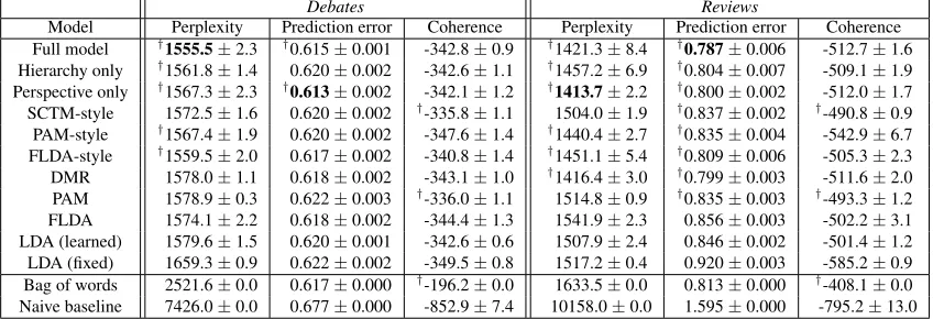
Debates Reviews
Model Perplexity Prediction error Coherence Perplexity Prediction error Coherence Full model †1555.5±2.3 †0.615±0.001 -342.8±0.9 †1421.3±8.4 †0.787±0.006 -512.7±1.6
Hierarchy only †1561.8
±1.4 0.620±0.002 -342.6±1.1 †1457.2
±6.9 †0.804
±0.007 -509.1±1.9 Perspective only †1567.3±2.3 †0.613±0.002 -342.1±1.2 †1413.7±2.2 †0.800±0.002 -512.0±1.7
SCTM-style 1572.5±1.6 0.620±0.002 †-335.8±1.1 1504.0±1.9 †0.837±0.002 †-490.8±0.9
PAM-style †1567.4±1.9 0.620±0.002 -347.6±1.4 †1440.4±2.7 †0.835±0.004 -542.9±6.7
FLDA-style †1559.5±2.0 0.617±0.002 -340.8±1.4 †1451.1±5.4 †0.809±0.006 -505.3±2.3
DMR 1578.0±1.1 0.618±0.002 -343.1±1.0 †1416.4±3.0 †0.799±0.003 -511.6±2.0
PAM 1578.9±0.3 0.622±0.003 †-336.0±1.1 1514.8±0.9 †0.835±0.003 †-493.3±1.2
FLDA 1574.1±2.2 0.618±0.002 -344.4±1.3 1541.9±2.3 0.856±0.003 -502.2±3.1 LDA (learned) 1579.6±1.5 0.620±0.001 -342.6±0.6 1507.9±2.4 0.846±0.002 -501.4±1.2 LDA (fixed) 1659.3±0.9 0.622±0.002 -349.5±0.8 1517.2±0.4 0.920±0.003 -585.2±0.9 Bag of words 2521.6±0.0 0.617±0.000 †-196.2±0.0 1633.5±0.0 0.813±0.000 †-408.1±0.0
[image:10.612.96.520.44.189.2]Naive baseline 7426.0±0.0 0.677±0.000 -852.9±7.4 10158.0±0.0 1.595±0.000 -795.2±13.0
Table 2: Perplexity of held-out tokens and mean absolute error for attribute prediction using various models (±std. error).
†indicates significant improvement (p <0.05) over optimized LDA under a two-sided t-test.
the prediction error using bag of words features, and we measure coherence of the unigram distri-bution; (2) naive baselines, where we measure the perplexity of the uniform distribution over each dataset’s vocabulary, the prediction error when simply predicting each attribute as the mean value in the training set, and the coherence of 20 ran-domly selected words (repeated for 10 trials).
Table 2 shows that the full SPRITEmodel
sub-stantially outperforms the LDA baseline at both predictive tasks. Generally, model variants with more structure perform better predictively.
The difference between SCTM-style and
PAM-styleis that the former uses only topic
com-ponents (for word distributions) and the latter uses only document components (for the topic distri-butions). Results show that the structured priors are more important for topic than word distribu-tions, since PAM-style has lower perplexity on both datasets. However, models with both topic and document components generally outperform
either alone, including comparing the
Perspec-tive onlyandDMRmodels. The former includes
both topic and document perspective components, while DMR has only a document level component.
PAM does not significantly outperform
opti-mized LDA in most measures, likely because it up-dates the hyperparameters using a moment-based approximation, which is less accurate than our
gradient-based optimization. FLDA perplexity
is 2.3% higher than optimized LDA onReviews,
comparable to the 4% reported by Paul and Dredze
(2012) on a different corpus. The FLDA-style
SPRITE variant, which is more flexible, signifi-cantly outperforms FLDA in most measures.
The results are quite different under the co-herence metric. It seems that topic components
(which influence the word distributions) improve coherence over LDA, while document compo-nents worsen coherence. SCTM-style (which uses only topic components) does the best in both datasets, while PAM-style (which uses only doc-uments) does the worst. PAM also significantly improves over LDA, despite worse perplexity.
TheLDA (learned)baseline substantially
out-performsLDA (fixed)in all cases, highlighting the
importance of optimizing hyperparameters, con-sistent with prior research (Wallach et al., 2009a).
Surprisingly, many SPRITEvariants also
outper-form the bag of words regression baseline, even though the latter was tuned to optimize
perfor-mance using heavy `2 regularization, which we
applied only weakly (without tuning) to the topic model features. We also point out that the “bag of words” version of the coherence metric (the co-herence of the top 20 words) is higher than the av-erage topic coherence, which is an artifact of how the metric is defined: the most probable words in the corpus also tend to co-occur together in most documents, so these words are considered to be highly coherent when grouped together.
Parameter Sensitivity We evaluated the full
model at the two predictive tasks with varying
numbers of topics ({12,25,50,100} for Debates
and {5,10,20,40} for Reviews) and components
({2,5,10,20}). Figure 5 shows that performance is more sensitive to the number of topics than com-ponents, with generally less variance among the latter. More topics improve performance
mono-tonically onDebates, while performance declines
at 40 topics onReviews. The middle range of
com-ponents (5–10) tends to perform better than too few (2) or too many (20) components.
2 5 10 20 1500
1600 1700 1800 1900
Per
ple
xity
Debates K=12
K=25
K=50
K=100
2 5 10 20 1400
1450 1500 1550
1600 Reviews
K=5
K=10
K=20
K=40
2 5 10 20
Number of components
.605 .610 .615 .620 .625 .630
Prediction
error
2 5 10 20
Number of components
[image:11.612.94.298.43.202.2].76 .80 .84 .88 .92
Figure 5: Predictive performance of full model with differ-ent numbers of topicsKacross different numbers of compo-nents, represented on the x-axis (log scale).
τt Debates Reviews
0.000 (Sparse DAG) 58.1% 42.4% 1.000 (Soft Tree) 93.2% 74.6%
1.001t (Hard Tree) 99.8% 99.4%
1.003t (Hard Tree) 100% 100%
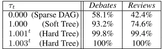
Table 3: The percentage of indicator values that are sparse (near 0 or 1) when using different annealing schedules.
choice of parameters may depend on the end ap-plication and the particular structures that the user has in mind, if interpretability is important. For example, if the topic model is used as a visual-ization tool, then 2 components would not likely result in an interesting hierarchy to the user, even if this setting produces low perplexity.
Structured Sparsity We use a relaxation of the
binarybthat induces a “soft” tree structure.
Ta-ble 3 shows the percentage ofbvalues which are
within = .001of 0 or 1 under various
anneal-ing schedules, increasanneal-ing the inverse temperature
τ by 0.1% after each iteration (i.e. τt = 1.001t)
as well as 0.3% and no annealing at all (τ = 1).
Atτ = 0, we model a DAG rather than a tree,
be-cause the model has no preference thatbis sparse.
Many of the values are binary in the DAG case, but the sparse prior substantially increases the number of binary values, obtaining fully binary structures with sufficient annealing. We compare the DAG and tree structures more in the next subsection. 7.3 Structure Comparison
The previous subsection experimented with mod-els that included a variety of structures, but did not provide a comparison of each structure in iso-lation, since most model variants were part of a complex joint model. In this section, we
exper-iment with the basic SPRITE model for the three
structures described in§3: a DAG, a tree, and a
factoredforest. For each structure, we also
exper-iment with each type of component: document,
topic, and both types (combined).
For this set of experiments, we included a third dataset that does not contain a perspective value:
• Abstracts:A set of 957 abstracts from the ACL
anthology (97,168 tokens; 8,246 types). These abstracts have previously been analyzed with FLDA (Paul and Dredze, 2012), so we include it here to see if the factored structure that we explore in this section learns similar patterns. Based on our sparsity experiments in the
pre-vious subsection, we set τt = 1.003t to induce
hard structures (tree and factored) andτ = 0to
in-duce a DAG. We keep the same parameters as the
previous subsection:K=50 andC=10 forDebates
andK=20 andC=5 forReviews. For the factored
structures, we use two factors, with one factor hav-ing more components than the other: 3 and 7
com-ponents forDebates, and 2 and 3 components for
Reviews(the total number of components across
the two factors is therefore the same as for the
DAG and tree experiments). TheAbstracts
exper-iments use the same parameters as withDebates.
Since theAbstractsdataset does not have a
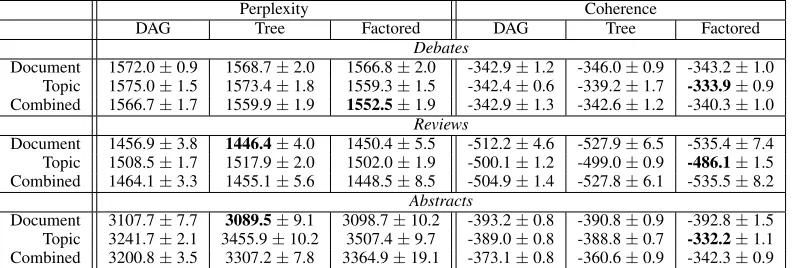
per-spective value to predict, we do not include predic-tion error as a metric, instead focusing on held-out perplexity and topic coherence (Eq. 2). Table 4 shows the results of these two metrics.
Some trends are clear and consistent. Topic components always hurt perplexity, while these components typically improve coherence, as was observed in the previous subsection. It has pre-viously been observed that perplexity and topic quality are not correlated (Chang et al., 2009). These results show that the choice of components depends on the task at hand. Combining the two components tends to produce results somewhere in between, suggesting that using both component types is a reasonable “default” setting.
[image:11.612.114.278.250.300.2]Perplexity Coherence
DAG Tree Factored DAG Tree Factored
Debates
Document 1572.0±0.9 1568.7±2.0 1566.8±2.0 -342.9±1.2 -346.0±0.9 -343.2±1.0 Topic 1575.0±1.5 1573.4±1.8 1559.3±1.5 -342.4±0.6 -339.2±1.7 -333.9±0.9 Combined 1566.7±1.7 1559.9±1.9 1552.5±1.9 -342.9±1.3 -342.6±1.2 -340.3±1.0
Reviews
Document 1456.9±3.8 1446.4±4.0 1450.4±5.5 -512.2±4.6 -527.9±6.5 -535.4±7.4 Topic 1508.5±1.7 1517.9±2.0 1502.0±1.9 -500.1±1.2 -499.0±0.9 -486.1±1.5 Combined 1464.1±3.3 1455.1±5.6 1448.5±8.5 -504.9±1.4 -527.8±6.1 -535.5±8.2
Abstracts
[image:12.612.111.508.42.176.2]Document 3107.7±7.7 3089.5±9.1 3098.7±10.2 -393.2±0.8 -390.8±0.9 -392.8±1.5 Topic 3241.7±2.1 3455.9±10.2 3507.4±9.7 -389.0±0.8 -388.8±0.7 -332.2±1.1 Combined 3200.8±3.5 3307.2±7.8 3364.9±19.1 -373.1±0.8 -360.6±0.9 -342.3±0.9 Table 4: Quantitative results for different structures (columns) and different components (rows) for two metrics (±std. error) across three datasets. The best (structure, component) pair for each dataset and metric is in bold.
factored structure tends to perform well under both metrics, with the lowest perplexity and highest co-herence in a majority of the nine comparisons (i.e. each row). Perhaps the models are capturing a nat-ural factorization present in the data.
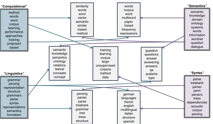
To understand the factored structure qualita-tively, Figure 6 shows examples of components from each factor along with example topics that draw from all pairs of these components, learned
on Abstracts. We find that the factor with the
smaller number of components (left of the figure) seems to decompose into components represent-ing the major themes or disciplines found in ACL abstracts, with one component expressing compu-tational approaches (top) and the other expressing linguistic theory (bottom). The third component (not shown) has words associated with speech, in-cluding{spoken,speech,recognition}.
The factor shown on the right seems to decom-pose into different research topics: one compo-nent represents semantics (top), another syntax (bottom), with others including morphology (top
words including{segmentation,chinese,
morphol-ogy}) and information retrieval (top words includ-ing{documents,retrieval,ir}).
Many of the topics intuitively follow from the components of these two factors. For example, the two topics expressing vector space models and distributional semantics (top left and right) both draw from the “computational” and “semantics” components, while the topics expressing ontolo-gies and question answering (middle left and right) draw from “linguistics” and “semantics”.
The factorization is similar to what had been previously been induced by FLDA. Figure 3 of Paul and Dredze (2012) shows components that look similar to the computational methods and linguistic theory components here, and the factor
with the largest number of components also de-composes by research topic. These results show
that SPRITEis capable of recovering similar
struc-tures as FLDA, a more specialized model. SPRITE
is also much more flexible than FLDA. While FLDA strictly models a one-to-one mapping of
topics to each pair of components, SPRITEallows
multiple topics to belong to the same pair (as in the semantics examples above), and conversely SPRITEdoes not require that all pairs have an
as-sociated topic. This property allows SPRITE to
scale to larger numbers of factors than FLDA, be-cause the number of topics is not required to grow with the number of all possible tuples.
8 Related Work
Our topic and perspective model is related to
su-pervised hierarchical LDA (SHLDA) (Nguyen et
al., 2013), which learns a topic hierarchy while also learning regression parameters to associate topics with feature values such as political per-spective. This model does not explicitly incorpo-rate perspective-specific word priors into the top-ics (as in our factorized approach). The regression
structure is also different. SHLDA is a
“down-stream” model, where the perspective value is a re-sponse variable conditioned on the topics. In
con-trast, SPRITE is an “upstream” model, where the
topics are conditioned on the perspective value. We argue that the latter is more accurate as a gen-erative story (the emitted words depend on the author’s perspective, not the other way around). Moreover, in our model the perspective influences both the word and topic distributions (through the topic and document components, respectively).
method! words! word! corpus! learning! performance! approaches! training! proposed! based! “Linguistics”! grammar! parsing! representation! structure! grammars! parse! syntax! representations! semantics! formalism! semantic! knowledge! domain! ontology! systems! words! information! wordnet! question! dialogue! parse! treebank! parser! penn! parsers! trees! dependencies! acoustic! corpus! parsing! training! learning! corpus! large! unsupervised! corpora! method! data! semantic! knowledge! semantics! ontology! relations! lexical! concepts! concept! similarity! words! word! vector! semantic! similar! based! method! words! corpus! word! multiword! paper! based! frequency! expressions! question! questions! answer! answering! answers! qa! systems! type! parsing! parser! parse! treebank! grammar! tree! trees! structure! german! languages! french! english! multilingual! italian! structure! spanish!
“Computational”! “Semantics”!
[image:13.612.136.481.38.239.2]“Syntax”!
Figure 6: Examples of topics (gray boxes) and components (colored boxes) learned on theAbstractscorpus with 50 topics using a factored structure. The components have been grouped into two factors, one factor with 3 components (left) and one with 7 (right), with two examples shown from each. Each topic prior draws from exactly one component from each factor.
topic-specific word distributions. This is an alter-native to the more common approach to regression based topic modeling, where the variables affect the topic distributions rather than the word
distri-butions. Our SPRITE-based model does both: the
document features adjust the prior over topic
dis-tributions (through δ), but by tying together the
document and topic components (withβ), the
doc-ument features also affect the prior over word dis-tributions. To the best of our knowledge, this is the first topic model to condition both topic and word distributions on the same features.
The topic aspect model (Paul and Girju, 2010a) is also a two-dimensional factored model that has been used to jointly model topic and perspective (Paul and Girju, 2010b). However, this model does not use structured priors over the parameters,
unlike most of the models discussed in§4.
An alternative approach to incorporating user preferences and expertise are interactive topic models (Hu et al., 2013), a complimentary ap-proach to SPRITE.
9 Discussion and Conclusion
We have presented SPRITE, a family of topic
mod-els that utilize structured priors to induce pre-ferred topic structures. Specific instantiations of SPRITE are similar or equivalent to several
exist-ing topic models. We demonstrated the utility of SPRITEby constructing a single model with many
different characteristics, including a topic hierar-chy, a factorization of topic and perspective, and
supervision in the form of document attributes. These structures were incorporated into the pri-ors of both the word and topic distributions, unlike most prior work that considered one or the other. Our experiments explored how each of these var-ious model features affect performance, and our results showed that models with structured priors perform better than baseline LDA models.
Our framework has made clear advancements with respect to existing structured topic models.
For example, SPRITE is more general and
of-fers simpler inference than the shared compo-nents topic model (Gormley et al., 2010), and SPRITEallows for more flexible and scalable
fac-tored structures than FLDA, as described in earlier sections. Both of these models were motivated by their ability to learn interesting structures, rather than their performance at any predictive task. Sim-ilarly, our goal in this study was not to provide state of the art results for a particular task, but to demonstrate a framework for learning struc-tures that are richer than previous structured mod-els. Therefore, our experiments focused on
un-derstanding how SPRITEcompares to commonly
used models with similar structures, and how the different variants compare under different metrics. Ultimately, the model design choice depends on the application and the user needs. By unifying
such a wide variety of topic models, SPRITEcan
Acknowledgments
We thank Jason Eisner and Hanna Wallach for helpful discussions, and Viet-An Nguyen for pro-viding the Congressional debates data. Michael Paul is supported by a Microsoft Research PhD fellowship.
References
D. Andrzejewski, X. Zhu, and M. Craven. 2009. In-corporating domain knowledge into topic modeling via Dirichlet forest priors. InICML.
R. Balasubramanyan and W. Cohen. 2013. Regular-ization of latent variable models to obtain sparsity. InSIAM Conference on Data Mining.
D. Blei and J. Lafferty. 2007. A correlated topic model of Science.Annals of Applied Statistics, 1(1):17–35.
D. Blei, T. Griffiths, M. Jordan, and J. Tenenbaum. 2003a. Hierarchical topic models and the nested Chinese restaurant process. InNIPS.
D. Blei, A. Ng, and M. Jordan. 2003b. Latent Dirichlet allocation.JMLR.
J. Chang, J. Boyd-Graber, S. Gerrish, C. Wang, and D. Blei. 2009. Reading tea leaves: How humans interpret topic models. InNIPS.
J. Duchi, E. Hazan, and Y. Singer. 2011. Adaptive sub-gradient methods for online learning and stochastic optimization.JMLR, 12:2121–2159.
J. Eisenstein, A. Ahmed, and E. P. Xing. 2011. Sparse additive generative models of text. InICML.
M.R. Gormley, M. Dredze, B. Van Durme, and J. Eis-ner. 2010. Shared components topic models. In
NAACL.
T. Griffiths and M. Steyvers. 2004. Finding scientific topics. InProceedings of the National Academy of Sciences of the United States of America.
Y. Hu, J. Boyd-Graber, B. Satinoff, and A. Smith. 2013. Interactive topic modeling. Machine Learn-ing, 95:423–469.
J. Kivinen and M.K. Warmuth. 1997. Exponentiated gradient versus gradient descent for linear predic-tors.Information and Computation, 132:1–63.
J.B. Lewis and K.T. Poole. 2004. Measuring bias and uncertainty in ideal point estimates via the paramet-ric bootstrap.Political Analysis, 12(2):105–127.
W. Li and A. McCallum. 2006. Pachinko alloca-tion: DAG-structured mixture models of topic cor-relations. InInternational Conference on Machine Learning.
D. Mimno and A. McCallum. 2008. Topic mod-els conditioned on arbitrary features with Dirichlet-multinomial regression. InUAI.
D. Mimno, W. Li, and A. McCallum. 2007. Mixtures of hierarchical topics with Pachinko allocation. In
International Conference on Machine Learning.
D. Mimno, H.M. Wallach, E. Talley, M. Leenders, and A. McCallum. 2011. Optimizing semantic coher-ence in topic models. InEMNLP.
V. Nguyen, J. Boyd-Graber, and P. Resnik. 2013. Lex-ical and hierarchLex-ical topic regression. InNeural In-formation Processing Systems.
M.J. Paul and M. Dredze. 2012. Factorial LDA: Sparse multi-dimensional text models. InNeural Informa-tion Processing Systems (NIPS).
M.J. Paul and M. Dredze. 2013. Drug extraction from the web: Summarizing drug experiences with multi-dimensional topic models. InNAACL.
M. Paul and R. Girju. 2010a. A two-dimensional topic-aspect model for discovering multi-faceted topics. InAAAI.
M.J. Paul and R. Girju. 2010b. Summarizing con-trastive viewpoints in opinionated text. InEmpirical Methods in Natural Language Processing.
M.J. Paul, B.C. Wallace, and M. Dredze. 2013. What affects patient (dis)satisfaction? Analyzing online doctor ratings with a joint topic-sentiment model. InAAAI Workshop on Expanding the Boundaries of Health Informatics Using AI.
M. Rabinovich and D. Blei. 2014. The inverse regres-sion topic model. InInternational Conference on Machine Learning.
D. Ramage, D. Hall, R. Nallapati, and C.D. Man-ning. 2009. Labeled LDA: a supervised topic model for credit attribution in multi-labeled corpora. In
EMNLP.
N.A. Smith and J. Eisner. 2006. Annealing structural bias in multilingual weighted grammar induction. In
COLING-ACL.
E.M. Talley, D. Newman, D. Mimno, B.W. Herr II, H.M. Wallach, G.A.P.C. Burns, M. Leenders, and A. McCallum. 2011. Database of NIH grants us-ing machine-learned categories and graphical clus-tering.Nature Methods, 8(6):443–444.
N. Ueda and R. Nakano. 1998. Deterministic anneal-ing EM algorithm. Neural Networks, 11(2):271– 282.
H.M. Wallach, D. Mimno, and A. McCallum. 2009a. Rethinking LDA: Why priors matter. InNIPS. H.M. Wallach, I. Murray, R. Salakhutdinov, and
D. Mimno. 2009b. Evaluation methods for topic models. InICML.
C. Wang and D. Blei. 2009. Decoupling sparsity and smoothness in the discrete hierarchical Dirich-let process. InNIPS.