A Low Complexity High Performance Bluetooth Receiver

A Low-Complexity High-Performance Bluetooth Receiver

Charles Tibenderana and Stephan Weiss Communications Research Group Department of Electronics & Computer Science

University of Southampton, UK

Email: ct02r,sw1 @ecs.soton.ac.uk

Abstract

This paper presents an implementation of a GFSK receiver based on matched filtering of a sequence of successive bits. This enables improved detection and superior BER

perfor-mance but requires matched filters of considerable complexity. Exploiting redundancy,

and performing phase propagation of successive single-bit stages, we propose a new re-ceiver structure of low complexity. Simulation results presented highlight the benefits of proposed method in terms of computational cost and performance compared to standard methods.

1.

Introduction

Software Defined Radios (SDR) perform signal processing tasks by running software algo-rithms on multi-purpose Digital Signal Processors (DSP). Flexibility offered by DSPs facilitate efficient integration of multiple standards, such as Bluetooth and WLAN, on a single radio sys-tem. For example, standard integration has been reported for Bluetooth with HiperLAN/2 [1, 2] and with IEEE 802.11b [3, 4]. As both HiperLAN/2 and 802.11b are considerably more com-plex than Bluetooth, a common hardware platform can provide extra computational power for the latter. This motivates to deviate from simplistic Bluetooth receivers to more sophisticated algorithms in order to achieve an improved system performance, whereby battery power con-sumption will benefit from an efficient realisation.

Therefore, this paper begins with a brief review of the Bluetooth modulation standard in Sec. 2, after which two possible realisations of a Bluetooth modulator are highlighted in Sec. 3. A low-complexity high-performance algorithm for Bluetooth demodulation is presented in Sec. 4, and evaluated in Sec. 5. Conclusions will be drawn in Sec. 6.

2.

Gaussian Frequency Shift Keying

The modulation scheme specified for Bluetooth is Gaussian Frequency Shift Keying (GFSK). GFSK is a form of Continuous Phase Frequency Shift Keying (CPFSK), which in turn is a varia-tion of Frequency Shift Keying (FSK). In binary FSK, equal amplitude sinusoidal waveforms at frequencies and are transmitted to signal bit 0 and 1 respectively, by switching

Discontinuities at symbol boundaries cause spurious transmissions, and poor bandwidth util-isation of FSK [5]. Spectral efficiency is improved in CPFSK, which constrains the phase of the transmitted signal to be continuous. This is achieved through FM modulation of a single carrier by a stream of binary data pulses. CPFSK is full response if the influence of a data pulse on the modulated signal does not exceed one bit period, otherwise it is partial response [6].

πh Integrator

N

exp()

ϕ[n] Rescale to

−1s and +1s filter ( K = 0.5)_BT

Data bits

b[k]

N

p[k] p[n] Gaussian

VCO

s[n] m[n]

Fig. 1: GFSK modulation. , and , are the bandwidth-time product, modulation index, and number of samples per symbol respectively.

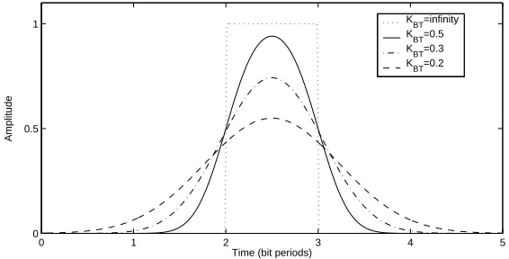
A GFSK modulator as portrayed in Figure 1, deploys a Gaussian filter prior to FM modu-lation to reduce the speed of frequency transitions and avoid discontinuities in the transmitted signal. The coefficients of the Gaussian pre-modulation filter are given by [7]

"!#$&%

(' *,+)

)/10

23!1#$&%

4' *5+)

)/087(9

(1)

where

is an integer,

is the ratio of the bit period to the sample period,

2"!;:3<>=

is the error function, and

%

? is the bandwidth-time product which is specified as 0.5 in the Standard [8].

for different values of

%

? are plotted in Figure 2.

0 1 2 3 4 5

0 0.5 1

Time (bit periods)

Amplitude

K

BT=infinity

K

BT=0.5

[image:2.595.74.524.145.209.2]

K_BT=0.3 K_BT=0.2

[image:2.595.156.439.419.563.2]

Fig. 2: Impulse response of a Gaussian filter,@AB?C.

Figure 3 shows how the Gaussian filter improves bandwidth utilisation, while Figures 4 and 2 illustrate that

%

? =0.5 results in a partial response signal with each bit affecting adjacent bit

periods.

The modulation index,D , defined as

D

)

E

9

(2) in which and E are the frequency deviation and bit period respectively [9], may vary in a

Bluetooth system betweenFHG )JILK

D

K

0 1 2 3 4 5 6 7 8 −1

−0.5 0 0.5 1

Time (bit periods)

m[ n ]

[image:3.595.157.439.56.197.2]

before filter after filter

Fig. 3: Effect of the Gaussian pre-modulation filter on the baseband pulse stream (

).

It follows that a GFSK modulated signal is given by

$

D

9

(3)

where

!

#"

!

%$

9

and

"

!'&)(

G

(4)

0 0.5 1

−1 −0.5 0 0.5 1

Time [ (n mod

N) / N ]

[image:3.595.159.443.259.544.2]

m[ n ]

Fig. 4: GFSK eye diagram of the instantaneous frequency signal* AB?C with

+ .

3.

Modulator

Figure 5 portrays a possible realisation of a Bluetooth modulator on a DSP. Incoming data is up-sampled by a factor of

, and then passed to an FIR filter with a Gaussian impulse response,

. The output of the Gaussian filter is multiplied by

,-. , and then an exponential function is

performed before each sample is multiplied by its predecessor to increment the phase of the transmitted signal.

In the above structure, convolution of

pulses with the

entails0/

multiply-accumulates in a bit period. The phase accumulator, and multiplication by

,1-. , will each consume

p[k] p[n] s[n]

N g[n] exp(j )

.

h

π

N

Fig. 5: Possible baseband implementation of a conventional GFSK modulator for a DSP.

multiplications, and 1 division per sample [10], or 22

operations per bit. The total computa-tional cost is

)

/

+

)

operations/bit.

An equivalent but more efficient modulator is portrayed in Figure 6. The lookup table con-tains 8 sequences of

samples each,

$

D

9

for

K

K

and

9

)

9

G2G;G

9

I

(5) where the sequences

represent the 8 different waveforms in Figure 4. Due to being partial response, the output

depends not only on the current bit, but also the preceding and fol-lowing one. Therefore, the serial-to-parallel converter in Figure 6 feeds 3 successive bit values into the look-up table, from which the correct instantaneous frequency signal segment

is determined. Multiplication of each of the lookup table output samples by the previous one accumulates the phase of the transmitted signal.

s[n]

P/S

N−samples

Look−up Table S/P

3−bits p[k]

Fig. 6: Efficient baseband GFSK modulator for a DSP.

In this model, all operations are achieved through indexing, except for the phase accumulator, which requires

operations per bit.

4.

Demodulator

A variety of demodulation and detection algorithms exist for Bluetooth. Relatively simple ones include FM-AM conversion, phase-shift discrimination, zero-crossing detection, and frequency feedback [11]. However, our project aims to integrate Bluetooth with IEEE 802.11b WLAN in an SDR. 802.11b is considerably more complex than Bluetooth, and so a common hard-ware platform can provide extra computational power for execution of Bluetooth. This is the motivation to deviate from simplistic Bluetooth receivers to more sophisticated algorithms. In order to achieve improved system performance, but to limit battery consumption by efficient implementation.

Hence, we adopt a high-performance demodulator structure, shown in Figure 7, which achieves the best possible performance in AWGN by utilising a bank of

)

FIR filters, matched to the

expected waveforms over a

%

processed, and a decision is made on the central bit. System performance improves with in-crease in

%

. In the diagram

)

, and the filters matched to waveforms

9 to 9

signal receipt of a bit .

s

0[ n , P ]Ψ

1

s [ n , P ]₁ s₀[ n , P ]₁

1

s [ n , P ]_Ψ

Nz1

z_Ψ N

NzΨ+1

Nz2Ψ

b[k] r[n]

Biggest Picker

Fig. 7: High performance CPFSK demodulator.

The high-performance CPFSK receiver is attractive for use in Bluetooth because of its en-hanced performance, and its ability to improve BER by increasing the observation interval,

%

. It is also suitable for integration with 802.11b, which also utilises a filter bank for demodu-lation [3, 4]. However, it is not popular because of its enormous complexity. For example, an observation interval of

%

bits will require

)

filters, each

%

taps long. Thus,

)

%

multiply-accumulates are required for filtering a bit worth of the received signal. Also,

)

multiplications and

)

additions are needed to compute the magnitude. This brings the number

of operations per bit to

) : % / = . !!!!! !!!!! !!!!! !!!!! !!!!! !!!!! !!!!! !!!!! !!!!! !!!!! !!!!! !!!!! !!!!! !!!!! !!!!! !!!!! !!!!! "" "" "" ## ## ## $$$ $$$ $$$ %%% %%% %%% &&&&& &&&&& &&&&& &&&&& &&&&& &&&&& &&&&& &&&&& ''''' ''''' ''''' ''''' ''''' ''''' ''''' ''''' ((((( ((((( ((((( ((((( )))) )))) )))) )))) ** ** ** ** ** ** ** ** ** ++ ++ ++ ++ ++ ++ ++ ++ ++ ,,,,, ,,,,, ,,,,, ,,,,, ,,,,, ,,,,, ,,,,, ----... ... ... ... /// /// /// /// 00000 00000 00000 00000 00000 00000 1111 1111 1111 1111 1111 1111 22 22 22 22 22 22 22 22 33 33 33 33 33 33 33 33 44444 44444 44444 44444 44444 44444 44444 44444 44444 55555 55555 55555 55555 55555 55555 55555 55555 55555 666 666 666 666 666 666 666 666 77 77 77 77 77 77 77 77 8888888888 8888888888 8888888888 8888888888 8888888888 8888888888 8888888888 8888888888 8888888888 8888888888 8888888888 8888888888 8888888888 9999999999 9999999999 9999999999 9999999999 9999999999 9999999999 9999999999 9999999999 9999999999 9999999999 9999999999 9999999999 9999999999 :::: :::: :::: :::: :::: :::: :::: ;;;; ;;;; ;;;; ;;;; ;;;; ;;;; ;;;; <<<<<<<< <<<<<<<< <<<<<<<< <<<<<<<< <<<<<<<< <<<<<<<< <<<<<<<< <<<<<<<< <<<<<<<< ======== ======== ======== ======== ======== ======== ======== ======== ======== >>>>> >>>>> >>>>> >>>>> >>>>> >>>>> >>>>> >>>>> >>>>> ???? ???? ???? ???? ???? ???? ???? ???? ???? @@@@@ @@@@@ @@@@@ @@@@@ @@@@@ @@@@@ @@@@@ @@@@@ @@@@@ @@@@@ @@@@@ @@@@@ AAAAA AAAAA AAAAA AAAAA AAAAA AAAAA AAAAA AAAAA AAAAA AAAAA AAAAA AAAAA BBB BBB BBB BBB BBB BBB BBB BBB CC CC CC CC CC CC CC CC DD DD DD EE EE EE FF FF FF GG GG GG

N taps only)

(8 Channels,

Filter Bank Biggest

[image:5.595.93.520.409.563.2]

Picker M1 2K b[k] S/P 3 r[n] M_K−1 8 M_K [k] z [k] y y[k−1] 2K y[k−K+1]

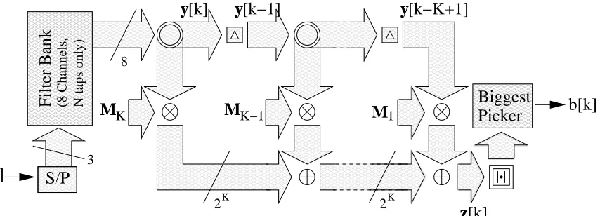
Fig. 8: Conceptual diagram of a low-complexity implementation of the high-performance GFSK demod-ulator for DSP.

The scheme in Figure 8 depicts the proposed low-complexity algorithm. In brief, the algo-rithm involves the use of a bank of 8 matched FIR filters with

coefficients spanning a single bit period, to filter each bit worth of received signal, and propagating the intermediate results,

H

$

, to finally obtain the

)

matched filter outputs,

I

$

. The filter result with the largest magnitude determines the received bit.

4.1 Filter Bank

The filter bank comprises of 8 matched FIR filters with

when

%

?

FGO The instantaneous frequencies of these waveforms were portrayed in Figure

4, and their modulated symbols were given in Equation 5. In the absence of carrier frequency mismatch, 4 of the filter bank entries are complex conjugate copies of the remaining ones, leading to a reduction in complexity by a factor of 2.

4.2 Matrices !

The last

%

sets of outputs from the filter bank are multiplied by matrices !

($

,

)

, G;G2G,

%

). Through these multiplications, the results for

)

filters with

%

coefficients covering

%

-bit span, are constructed.

!

are

)

by 8 matrices with

)

non-zero elements, which effect

a permutation and phase shift on the intermediate outputs from the filter bank,

$

, (where

=

9

)

9

G;G;G

9

I

, and = F

9

)

9

G;G;G

9

%

[image:6.595.157.437.296.535.2]

).

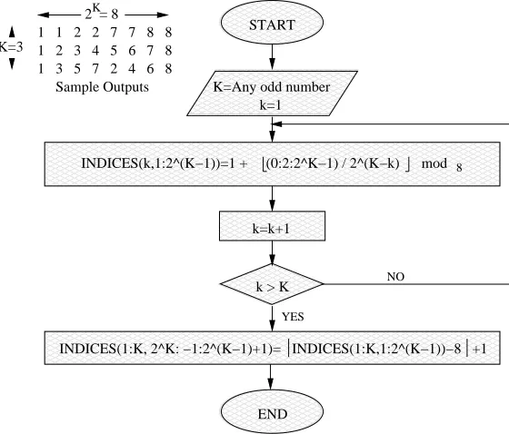
Figure 9 contains a flow graph for an algorithm that can be used to compute the positions of the non-zero elements of !

, off-line, for arbitrary

%

, while Figure 10 computes their values. In both cases, coefficients of filter 1 to 8, emanate from modulation of the middle pulse in

sequences

to

respectively.

INDICES(1:K, 2^K: −1:2^(K−1)+1)= INDICES(1:K,1:2^(K−1))−8 +1 Sample Outputs

1 2 3 4 5 6 7 8 K=3

1 1 2 2 7 7 8 8

1 3 5 7 2 4 6 8

K

2 = 8

k=k+1

8

INDICES(k,1:2^(K−1))=1 + (0:2:2^K−1) / 2^(K−k) mod

END k > K

YES

k=1 K=Any odd number

START

NO

Fig. 9: Algorithm to determine the position of the non-zero elements of matrices

!

.

4.3 Example

$

<

H

$

/

<

H

$

<

H

$

)

(6) An example in which

%

M is considered here. In this case, the algorithm is summarised by

Equation 6 in whichH

$

,H

$

, andH

$

)

are vectors whose elements are the intermediate results depicted in Equation 7,I

$

is a vector containing the final outputs given in Equation 8, and , / , and

are the matrices in Equations 9, 10 and 11 respectively.

H

$

$

.. .

$

K=Any odd number

n=1

VALUES=ones(2 ,K)K

n = n + 1 START

m = 2

m = m + 1

k > 1 2K= 8

* s [N] 1 1 1 1 1 1 1 1 * s [N] * s [N] * s [N] 1 * s [N] * s [N] * s [N] * s [N] * s [N] K=3 * s [N] * s [N] * s [N] 5 6 7 * s [N] * s [N] * s [N] * s [N] * s [N] s [N] s [N] s [N] s [N] 4 4 3 5 * s [N] * 8 Sample Outputs . . . . . . . . 1 1 * s [N] 2 2 3 3 2 6 7 8 2 3 4 1 * * * * 4

j_θ8

exp( )

j_θ2

exp( )

j_θ1

exp( )

s [N]

1

S = *

* s [N] s [N] 2 * 8 =

k = k − 1

m = k

K

n = 2

END YES NO YES NO NO YES

VALUES(m , n)= INDICES( m, n ) S(INDICES( k−1, n) ) s [N]

.

Fig. 10: Algorithm to determine the values of the non-zero elements of matrices

! . I $ .. . $ (8)

F F F F F F F

F F F F F F F

F

F F F F F F

F

F F F F F F

F F F F F F

F

F F F F F F

F

F F F F F F F

F F F F F F F

(9) /

F F F F F F F

F

!!

F F F F F F

F F

#"

F F F F F

F F F

!$"

F F F F

F F F F

#%

F F F

F F F F F

$%

F F

F F F F F F

'&

F

F F F F F F F

/

!

F F F F F F F

F F

!

#"

F F F F F

F F F F

$"

F F F

F F F F F F

#"

F

F

$%

F F F F F F

F F F

$%

F F F F

F F F F F

&

%

F F

F F F F F F F

/

&

(11)

For example,

$

is given by

$"

<

$

#"

<

$

/

$

)

(12)

The computational complexity per bit, of the efficient demodulator is as follows: 4

multiply-accumulates are needed to calculateH

$

once per bit,

I

: %

=

multiplications are required to impose the phase shifts, after which

I

: %

=

additions are performed to obtain the final outputs, I

$

. Magnitude calculations consume

)

multiplications and

)

additions. This

totals up to /

)

I

: %

=

operations/bit.

5.

Simulation Results

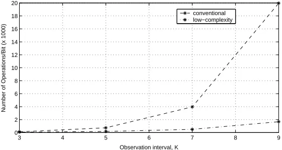
The computational complexities of a conventional and efficient implementation of a Bluetooth modem as a function of the observation interval

%

, and the number of samples per bit

, are given in Table 1, and plotted in Figure 11. Complexity is evaluated in operations/bit, whereby multiplication or addition involve one operation, while division requires 16 operations. These illustrations show that complexity rises less rapidly with increase in

%

in the efficient case. method parameters complexity (operations/bit) SNR at BER=

F

conventional

%

9

)

14 20dB

[12, 13, 14]

%

9

)

)

:

/

%

=

19968 11dB

proposed

%

9

)

/

)

I

:%

=

1680 11dB

Tab. 1: Comparison of complexity and SNR performance of conventional and proposed GFSK detectors.

The bit error ratio (BER) performances of the conventional and efficient implementations are the same, and their performance improves with a larger

%

[12]. Hence, BER improvements offered by the low-complexity realisation in an SDR will be attained by increasing

%

. For example, if the computing power available on the DSP was limited to 2000 operations per bit period, then the conventional method would only support a receiver based on

%

O successive

bit periods, while the efficient implementation can afford

%

, as see in Figure 11). The resulting BER performance of the two systems are displayed in Figure 12; the efficient method has 1.2 dB improvement at a BER of

F

.

In both cases, the performance of the high-performance receiver is better than the demodu-lation algorithms in [2], the best of which attained a BER of

F

3 4 5 6 7 8 9 0

2 4 6 8 10 12 14 16 18 20

Observation interval, K

Number of Operations/Bit (x 1000)

[image:9.595.157.437.55.204.2]

conventional low−complexity

Fig. 11: Computation complexity: Conventional vs. low-complexity with N=2.

0 2 4 6 8 10 12 14

10−4 10−3 10−2 10−1 100

Eb/No (dB)

BER

[image:9.595.161.438.243.391.2]

conventional, K=5 low−complexity, K=9

Fig. 12: BER performance curves of the modems with a limit of 2000 operations per bit for parameters

, and

6.

Conclusion

The maximum permissible BER for a Bluetooth system is

F

[8]. Schiphorst et al.

demon-strated that the best of the comparatively simple algorithms mentioned above achieve accept-able performance above a channel SNR of 14.8 dB, while some practitioners assume a channel SNR of 21 dB [16] to attain the minimum Bluetooth performance requirement. By using a high-performance demodulator described in [12, 13, 14, 15], where decisions are based on an observation interval spanning

%

bit periods, a BER of

F

is reached at a channel

SNR of 11 dB (as demonstrated in Figure 12). The 3.8 dB gain achieved with this technique is substantial, and yet the high-performance demodulator is not popular because of enormous computational requirements for large

%

A common hardware platform for IEEE 802.11b WLAN and Bluetooth will have extra ca-pacity to improve Bluetooth performance. Since it might not necessarily have the computational capacity to handle a high-performance demodulator with sufficiently large observation intervals, the efficient high-performance algorithm described in this paper helps to considerably reduce the computational requirements. As demonstrated in an example for

%

7.

References

[1] Roel Schiphorst, Fokke Hoeksema, and Kees Slump, “Channel Selection Requirements for Blue-tooth Receivers using a Simple Demodulation Algorithm ,” in Proceedings of ProRISC 2001, Veldhoven, Netherlands, November 2001, pp. 584–591.

[2] Roel Schiphorst, Fokke Hoeksema, and Kees Slump, “Bluetooth Demodulation Algorithms and their Performance,” in Proc. 2nd Karlsruhe Workshop on Software Radios, Karlsruhe, March 2002, pp. 99–105.

[3] Charles Tibenderana, Terence E. Dodgson, Stephan Weiss, and Derek Babb, “Towards Software Defined Radio (SDR) Bluetooth and IEEE 802.11b Modem Integration,” in 9th Wireless World

Research Forum Meeting, Zurich, July 2003.

[4] Charles Tibenderana and Terence E. Dodgson, “Integrated modulators and demodulators,” UK Patent Application 0219740.8, Samsung Electronics Research Institute, Stains, August 2002.

[5] Theodore S. Rappaport, Wireless Communications: Principles and Practice, Prentice Hall, New Jersey, July 1999.

[6] John B. Anderson, Tor Aulin, and Carl-Erik Sundberg, Digital Phase Modulation, Plenum Press, New York and London, 1986.

[7] Raymond Steele and Lajos Hanzo, Mobile Communications, John Wiley and Sons, West Sussex, 2nd edition, 1999.

[8] Bluetooth Special Interest Group, Specification of the Bluetooth System, February 2002, Core.

[9] Rudi De Buda, “Coherent Demodulation of Frequency-Shift Keying With Low Deviation Ratio,” in Proc. International Conference on Communications, Montreal, June 1971, pp. 429–435.

[10] Erwin Kreyszig, Advanced Engineering Mathematics, John Wiley and Sons, New York, 6th edition, 1988.

[11] Bruce A. Carlson, Communication Systems, McGraw-Hill, Singapore, 3rd edition, 1986.

[12] William P. Osborne and Micheal B. Luntz, “Coherent and Noncoherent Detection of CPFSK,” in

IEEE Transactions on Communications, August 1974, vol. COM-22, pp. 1023–1036.

[13] Thomas A. Schonhoff, “Symbol Error Probabilities for M-ary CPFSK: Coherent and Noncoherent Detection,” in IEEE Transactions on Communications, June 1976, vol. COM-24, pp. 644–652.

[14] W. Hirt and S. Pasupathy, “Suboptimal Reception of Binary CPSK Signals,” in Proc. IEE

Commu-nications, Radar and Signal Processing, United Kingdom, June 1981, vol. 128, pp. 125–134.

[15] John G. Proakis, Digital Communications, McGraw-Hill, New York, 3rd edition, 1995.