Gait Parameter and Speed Estimation from the
Frontal View Gait Video Data Based on the Gait
Motion and Spatial Modeling
Kosuke Okusa and Toshinari Kamakura
Abstract—We study the problem of analyzing and classifying frontal view gait video data. In this study, we suppose that frontal view gait data as a mixing of scale changing, human movements and speed changing parameters. We estimate these parameters using the statistical registration and modeling on a video data. Our gait model is based on human gait structure and temporal-spatial relations between camera and subject. To demonstrate the effectiveness of our method, we conducted two sets of experiments, assessing the proposed method in gait analysis for young/elderly person and abnormal gait detection. In abnormal gait detection experiment, we apply K-nearest-neighbor classifier, using the estimated parameters, to perform normal/abnormal gait detect, and present results from an experiment involving 120 subjects (young person), and 60 subjects (elderly person). As a result, our method shows high detection rate.
Index Terms—Gait Analysis, Human Gait Modeling, Statis-tical Registration, Abnormal Gait Detection
I. INTRODUCTION
W
E study the problem of analyzing and classifying frontal view gait video data. A study on the human gait analysis is very important in the field of the sports/health managements. For instance, gait analysis is one of the important method to detect the Alzheimer disease, infantile paralysis, and any other diseases [1], [2], [3].Gait analysis is mainly based on motion capture system and video data. The motion capture system can give the precise measurements of trajectories of moving objects, but it requires the laboratory environments and we cannot be used this system in the field study. On the other hand, the video camera is handy to observe the gait motion in the field study. Gage [4] had been proposed brain paralysis gait analysis using gait video data. Kadaba et al.[5] had been discussed importance of lower limb in the human gait using gait video data too. Many gait analysis have recently analyzing using video analysis software (e.g. Dartfish, Contemplas, Silicon Coach). For example, Borelet al.[6] and Gruntet al.[7] had been proposed infantile paralysis gait analysis using lateral view gait video data.
On the other hand, from the standpoint of statistics, Olshen
et al. [8] proposed the bootstrap estimation for confidence intervals of the functional data with application to the gait cycle data observed by the motion capture system. Sorianoet al.[9] proposed the human recognition method based on the data matching techniques using the dynamic time warping of human silhouettes.
K. Okusa is with the Department of Science and Engineering, Chuo University, Tokyo, 1128551 Japan e-mail: [email protected].
T. Kamakura is with the Department of Science and Engineering, Chuo University, Tokyo, 1128551 Japan e-mail: [email protected].
However, most studies have not focused on frontal view gait analysis, because such data has many restrictions on analysis based on the filming conditions. The video data filmed from the frontal view is difficult to analyze, because the subject getting close in to the camera, and data includes the scale-changing parameters [10], [11]. To cope with this, Okusa et al. [12] and Okusa & Kamakura [13] proposed a registration for scales of moving object using the method of nonlinear least squares, but Okusaet al.[12] and Okusa & Kamakura [13] did not focus on the human leg swing.
Okusa & Kamakura [14] focus on the gait analysis using arm and leg swing model estimated parameters. However, their work was not enough to describe and verification about further details of human gait and spatial modeling and its parameter and speed estimation. In this paper, we describe further details and verification about Okusa & Kamakura [14] models and its applications.
In this study, we focus on the gait analysis using arm and leg swing model estimated parameters. We suppose that frontal view gait data as a mixing of scale changing, human movements and speed changing parameter. We estimate these parameters using the statistical registration and modeling on a video data. Our gait model is based on the human gait structure and temporal-spatial relations between camera and human.
To demonstrate the effectiveness of our method, we con-ducted two sets of experiments, assessing the proposed method in gait analysis for young/elderly person and abnor-mal gait detection.
In young/elderly gait analysis experiment, we analyze young 120 subjects and elderly 60 subjects (normal gait: 46, abnormal gait: 14). We discuss the normal and abnormal gait features using the estimated parameters from proposed model. In abnormal gait detection experiment, we apply a K-nearest-neighbor (K-NN) classifier, using the estimated parameters, to perform abnormal gait detection, and present results from an experiment involving 180 subjects from young/elderly gait analysis. As a result, our method shows high detection rate.
The organization of the rest of the paper is as follows. In Section II, we discuss the advantage and problem of frontal view gait analysis. In Section III, we present our models for frontal view gait data based on the statistical registration and gait modeling. In Section IV, we present some performance results showing the effectiveness of our models, based on applying proposed models to 180 subjects gait data. We conclude with a summary in Section V.
IAENG International Journal of Applied Mathematics, 43:1, IJAM_43_1_05
II. FRONTALVIEWGAITDATA
In this section, we describe an overview of frontal view gait data. Many of gait analysis using lateral view gait data, because lateral view gait is easy to detect the human gait features. However, in a corridor like structure, the subject is approaching a camera. Such case is difficult observe lateral view gait.
In a lateral view gait, at least two cycles or four steps are needed. For more robust estimation of the period of walking, about 8m is recommended. To capture this movement, the camera distance required is about 9m. Practically, having such a wide space is difficult. On the other hand, frontal view gait video is easy to observe 8m (or more) gait steps [11].
[image:2.595.310.527.74.275.2]Figure 1 is an example of frontal view gait data recorded by Figure 2 situation. Figure 1 illustrates difficulty of frontal view gait analysis. Even if subject do the same motion with the same timing, frontal view gait data is included scale changing components. Figure 3 shows subject width time-series behavior of frontal view gait data. This figure illustrates frontal view gait data contains many time-series components.
[image:2.595.50.291.331.392.2]Fig. 1. Frontal view gait data
Fig. 2. Filming situation of frontal view gait data
III. MODELING OF FRONTAL VIEW GAIT DATA A. Preprocessing
The raw video data is difficult to observe subject width and height time-series behavior because data contain background. We separate subject from background using inter-frame sub-traction method (Eq. 1).
∆(T)=|I(T+1)−I(T)|, T = 1, ...,(n−1),
∆(T)(p, q) =
{
1 (∆(T)(p, q)>0)
0 (Otherwise). (1)
Here, ∆(T) is an inter-frame subtraction image, I(T) is grey scaled video data image at frameT,(p, q)is the pixel coordinate.
0 1 2 3 4 5
60
80
100
120
140
Time
Width (pixel)
Fig. 3. Time-series behavior of frontal view subject width
a) Subject Width/Height Calculation: Inter-frame sub-traction method can separate the subject and background. However, it is difficult to measure the time-series behavior of the subject width and height. In this section, we describe the subject width and height calculation method using inter-frame subtraction data.
Let us suppose that inter-frame subtraction image is binary matrix. We can measure the subject height and width by integration calculation of row and column at each frame. In this study, we focus on the human gait arm and leg swing of the frontal view gait. We assume that subject width and height time-series behavior consist of the arm and leg swing behavior.
[image:2.595.57.271.420.560.2]B. Relationship between camera and subject
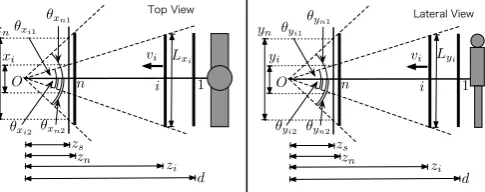
Figure 4 shows a relationship between camera and subject. Width and height modeling has same structure. In this section, we describe the subject width modeling. We can assume simple camera structure. We consider the virtual screen exists between observation point and subject, and we define subject width on the virtual screen xi at i-th frame(i= 1, ..., n).
i 1
O
vi
zs zn
zi d n
xi xn
i 1
O
vi
zs zn
zi d n
yi yn
Top View Lateral View
Lxi Lyi
θxi1
θxi2 θxn2 θxn1
θyi1
θy
i2 θyn2
θy
n1
Fig. 4. Relationship between camera and subject
Here we define zi, zj as distance between observation point and subject ati-th, j-th frame,zsas distance between observation point and virtual screen, θxi1, θxi2 as subject angle of view from observation point at i-th frame, d as
IAENG International Journal of Applied Mathematics, 43:1, IJAM_43_1_05
[image:2.595.307.550.605.701.2]distance between observation point and 1st frame, vi as subject speed at i-th frame. Okusa et al. [12] defined the subject length L was constant. We assume that L has the time-series behavior and we define Li is the subject length ati-th frame.
xi ati-th frame depends onθxi1,θxi2 as shown in Figure 4.
xi=zs(tanθxi1+ tanθxi2). (2) Similarly, the subject length at i-th frame is
Lxi =zi(tanθxi1+ tanθxi2). (3) From Eq.(2), Eq.(3), ratio between xn andxi is
xn xi
= Lxnzi Lxizn
(4)
Frame interval is equally-spaced (15 fps). Okusaet al.[12] assumed the average speed is constant. We can assume that average speed from i-th frame is (n−i) = (zi−zn)/¯v , thereforeziiszi=zn−v¯(n−i). We substitutezi to Eq.(4)
xi=
Mxiγ
γ+ (n−i)xn+i, (5)
whereγis zn/v¯,Mxi is Lxi/Lxn,iis noise. From Eq.(5),
predicted value xˆ(in) is registration from i-th frame’s scale ton-th frame’s scale
ˆ
x(in)= γ+ (n−i)
Mxiγ
xi. (6)
Similarly, we can define subject height as
yi=
Myiγ
γ+ (n−i)yn+i, (7)
whereMyi is Lyi/Lyn.
Next, we discuss the scale changing, human movement, and speed changing parameter estimation model.
C. Scale changing parameter estimation
From Eq.(5), scale parameter is γ. Solve Eq.(5) for γ
shows
γ= xi(n−i)
xi−Mxixn
. (8)
Here γ is the ungaugeable parameter, and we estimate it using nonlinear least squares method
S(γ, Mxi) =
n ∑
i=1
{ xi−
Mxiγ γ+ (n−i)xn
}2
. (9)
D. Human movement parameter estimation
Mxi andMyi are movement model of the subject. If the
subject is the rigid body, movement modelMxi andMyi are
constant. Meanwhile, human gait is not a constant.Mxi and Myi needs the movement model because the subject body is
moving wildly.
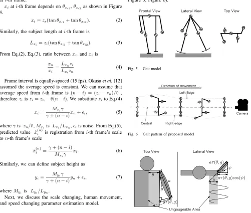
b) Human gait modeling: arm swing: Collinset al.[15] has reported that arm swing is an very important role in the gait motion based on the simple gait model. We consider the human gait modeling based on Collinset al.[15] model (see Figure 5, Figure 6).
Frontal View Lateral View Top View
[image:3.595.48.550.110.535.2]Fig. 5. Gait model
Fig. 6. Gait pattern of proposed model
θ
g
Ungaugeable Area Top View Lateral View
aτ(θ, g)
aτ(θ, g) ψ
g
a
[image:3.595.314.540.407.531.2]aτ(θ, g)cos(ψ)
Fig. 7. Arm swing model
It seems reasonable to think that arm is single pendulum. Collinset al.[15] model assumed the arm swing is move to anteroposterior direction. Our model, on the other hand, can assume that arm swing move to an oblique direction (Figure 7).
Figure 7’s model has an ungaugeable area. Our method’s width/height calculation is based on integration calculation of row and column at each frame. If the arm move to inside body area, arm length is ungaugeable. Arm swing model is
xi= (
W(P1,P2,Q1,Q2,g1,g2,f,i)
W(P1,P2,Q1,Q2,g1,g2,f,n)+s
) γ
γ+ (n−i) xn+i
W(P1, P2, Q1, Q2, g1, g2, f, i) =
P1τ(f i+Q1, g1) +P2τ(f i+Q2, g2)
τ(θ, g) =
{
sin(θ) +g (sin(θ) +g >0)
0 (Otherwise) (10)
IAENG International Journal of Applied Mathematics, 43:1, IJAM_43_1_05
where P1 = a1cos(ψ) and P2 = a2cos(ψ). P1τ(f i+
Q1, g1) andP2τ(f i+Q2, g2)are right and left arm model respectively. From Eq.(10), we estimate each gait parameter using nonlinear least squares method.
S(γ, P1, P2, Q1, Q2, g1, g2, f, s) = n
∑
i=1
{ xi−
(
W(P1,P2,Q1,Q2,g1,g2,f,i)
W(P1,P2,Q1,Q2,g1,g2,f,n)+s
) γ
γ+ (n−i) xn
}2 (11)
Here,f is gait cycle frequency,sis adjustment parameter,
P1, P2are arm swing amplitude parameters,Q1, Q2 are arm phase parameters, and g1, g2 are ungaugeable area parame-ters.
c) Human gait modeling: leg swing: The leg swing modeling is simpler than arm swing model because the leg model does not have a ungaugeable area. Okusa et al.[12] and Okusa & Kamakura [13] does not consider the leg swing. It seems reasonable to think like arm swing that leg swing is single pendulum (Figure 8).
bcos(ω)
ω
[image:4.595.313.548.98.451.2]b
Fig. 8. Leg swing model
Leg swing model is
yi= (
H(b1,Q3,f,i)
H(b1,Q3,f,n)+s
) γ
γ+ (n−i) yn+i
H(b1, Q3, f, i) =b1cos(f i+Q3). (12) Here b1 is leg swing amplitude parameter, andQ3 is leg phase parameter.
E. Speed changing parameter estimation
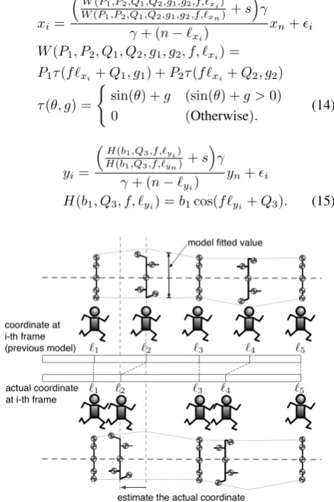
Frontal view video data is difficult to see the subject’s speed. If our gait model is correct, observed valuexiandyi is same as the fitted value of gait model at point`i. Previous model’s `i assumes equally spaced (`i =i = 1, ..., n). We estimate `xi and`yi value for minimize the observed value
and model fitted value at `i. We can define estimated value `xi and`yias a virtual space coordinate at i-th frame (Figure
9).
Eq.5, Eq.7 with the coordinate estimation shows
xi =
Mxiγ γ+ (n−`xi)
xn+i yi=
Myiγ γ+ (n−`yi)
yn+i. (13)
Here, `xi, ..., `xn and `yi, ..., `yn are virtual space
coor-dinate parameters of width and height respectively. From
Eq.13, arm swing and leg swing model with the coordinate estimation shows Eq.14, Eq.15.
xi= (W(P
1,P2,Q1,Q2,g1,g2,f,`xi)
W(P1,P2,Q1,Q2,g1,g2,f,`xn)+s )
γ
γ+ (n−`xi)
xn+i W(P1, P2, Q1, Q2, g1, g2, f, `xi) =
P1τ(f `xi+Q1, g1) +P2τ(f `xi+Q2, g2) τ(θ, g) =
{
sin(θ) +g (sin(θ) +g >0)
0 (Otherwise). (14)
yi= (H(b
1,Q3,f,`yi)
H(b1,Q3,f,`yn)+s )
γ
γ+ (n−`yi)
yn+i
[image:4.595.45.284.309.521.2]H(b1, Q3, f, `yi) =b1cos(f `yi+Q3). (15)
Fig. 9. Virtual space coordinate estimation
We suppose that virtual space coordinate of subject is
ˆ
`i= (ˆ`xi+ ˆ`yi)/2. Then, we can assume that subjects speed
is 1st order difference of `ˆi, and acceleration is 2nd order difference of`ˆi.
We estimate these models parameters using Okusa & Kamakura [16] method. This method is very stable and very fast to estimate these parameters.
F. Gait parameter estimation
In this section, we discuss the gait parameter estimation. We took movie of 10 subjects walking video data from frontal view (10 steps, Male, average height: 176.4cm, sd: 3.07cm) and apply to our proposed method. To validate the effectiveness of Eq.14 & Eq.15 model, we observe the gait acceleration of hip at the same time. We use Wireless Technology WAA-006 acceleration/angular velocity sensor.
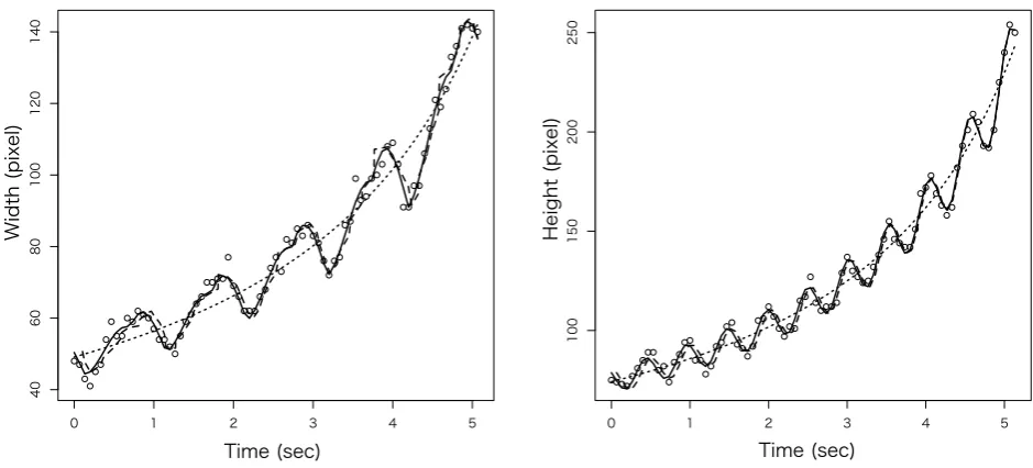
Figure 10(a) (left side) is plot of the subject width(pixel) time-series behavior. Here dotted line represent fitted value of Eq.5 (scale variant estimation model), continuous line represent fitted value of Eq.10 (scale variant + arm move-ments estimation model), dashed line represent fitted value of Eq.14 (scale variant + arm movements + speed variant estimation model). Similarly, Figure 10(a) (right side) is plot of the subject height(pixel) time-series behavior. Here dotted
IAENG International Journal of Applied Mathematics, 43:1, IJAM_43_1_05
Time(sec)
W
idth
(pixel)
0 1 2 3 4 5
40
60
80
100
120
140
Time (sec)
H
eight
(pixel)
0 1 2 3 4 5
100
150
200
250
(a) Model fitting: width (left side), height (right side)
Time (sec)
Acceleration
(
m
se
c
2 )
0 1 2 3 4 5
0.0
0.1
0.2
0.3
Time (sec)
Acceleration
(
fr
am
e
se
c
2
)
0 1 2 3 4 5
-0.6
-0.4
-0.2
0.0
0.2
0.4
[image:5.595.57.527.54.267.2](b) Observed acceleration (left side) and estimated acceleration (right side) Fig. 10. Fitted value and estimated acceleration
line represent fitted value of Eq.7 (scale variant estimation model), continuous line represent fitted value of Eq.12 (scale variant + leg movements estimation model), dashed line represent fitted value of Eq.15 (scale variant + leg movements + speed variant estimation model).
Figure 10(b) (left side) is observed acceleration of hip and 10(b) (right side) is estimated acceleration from Eq.14 and Eq.15 model. Eq.14 and Eq.15 model can not estimate acceleration scale, because estimated acceleration is second order difference of`ˆi. However, from Figure 1, we think our proposed model can estimate gait cycle and its timings.
Table I is Residual Sum of Squares (RSS), Akaike mation Criterion (AIC) [17] and Consistent Akaike’s Infor-mation Criterion (cAIC) [18] value of first order regression, second order regression, Eq.5 and Eq.7, Eq.10 and Eq.12, and Eq.14 and Eq.15 models of width and height data.
In Table I, most minimal AIC model is Eq.10, Eq.12.
Meanwhile, most minimal RSS and cAIC model are Eq.14, Eq.15. Burnham & Anderson [19] strongly recommend using cAIC, rather than AIC, if number of data n is small or number of parameters k is large. Since cAIC converges to AIC as n gets large, cAIC generally should be employed regardless. Therefore, we select the Eq.14, Eq.15 model. Figure 10(a), 10(b) and Table I illustrates our method has a good performance.
In next section, we discuss the effectiveness of our method.
IV. EXPERIMENTALDETAILS ANDRESULTS
To demonstrate the effectiveness of our method, we con-ducted two sets of experiments, assessing the proposed method in gait analysis for young/elderly person and abnor-mal gait detection. We use SONY DCR-TRV70K camera. Frame rate of video data is 15 fps and resolution is640×480.
IAENG International Journal of Applied Mathematics, 43:1, IJAM_43_1_05
[image:5.595.53.533.70.529.2] [image:5.595.57.528.311.530.2]TABLE I
RSS, AIC,CAICVALUE OF WIDTH AND HEIGHT DATA
Subject ID
Model Method A B C D E F G H I J
1st order RSS 9428.58 8051.10 5141.30 6834.98 8659.38 5882.43 3231.88 3867.81 7402.96 3695.14 regression AIC 607.97 601.95 541.97 569.94 627.29 558.38 501.09 508.77 607.95 545.31 cAIC 608.03 602.00 542.02 569.99 627.34 558.44 501.15 508.83 608.00 545.36 2nd order RSS 5260.57 2175.70 1654.54 3808.77 3250.35 1190.80 912.90 2062.37 2395.75 2909.74 regression AIC 563.88 499.28 457.80 526.91 547.96 437.39 408.28 464.24 517.43 527.96 cAIC 564.04 499.43 457.96 527.08 548.11 437.55 408.44 464.41 517.59 528.11 Eq.5 & Eq.7 RSS 5271.18 1367.39 1888.35 3077.40 2707.40 891.99 706.91 2052.45 2062.45 2865.62 model AIC 562.04 460.12 465.85 508.50 530.79 413.14 387.10 461.88 503.15 524.72 cAIC 564.19 462.28 468.01 510.66 532.94 415.30 389.26 464.05 505.30 526.88 Eq.10 & Eq.12 RSS 174.52 94.46 112.06 425.63 306.59 286.70 65.99 87.02 0.40 0.56 model AIC 308.81 262.32 267.19 372.17 366.00 341.74 225.25 244.00 -180.87 -150.70 cAIC 311.42 264.90 269.91 374.86 368.46 344.43 228.02 246.81 -178.37 -148.17 Eq.14 & Eq.15 RSS 84.31 33.02 60.49 189.46 95.82 149.21 61.39 27.33 0.02 0.10 model AIC 409.33 338.23 372.33 463.84 435.47 445.45 369.83 306.29 -258.9562 -130.86 cAIC -1157.07 -1263.77 -1089.67 -1032.56 -1275.73 -1050.95 -1058.17 -1088.11 -1896.956 -1768.86
Number of frames: 79 80 76 77 83 77 75 74 81 79
In this paper, we focus on γˆ (speed parameter), ( ˆP1+
ˆ
P2)/2(width amplitude parameter), andˆb1(height amplitude parameter).
A. Gait analysis: young person
In this experiment we took movie of 120 subjects walking video data from frontal view (10 steps, Male: 96 (aver-age height: 173.24cm, sd: 5.64cm), Female: 24 (aver(aver-age height:156.25cm, sd: 3.96cm)) and apply to our proposed method for the gait analysis.
0.5 1.0 1.5 2.0
30
40
50
60
70
80
90
Width amplitude
Speed
Fig. 11. Width amplitude vs speed (young)
Figure 11, 12 are width amplitude vs speed and height amplitude vs speed. The important point to note is that speed parameterˆγiszn/v¯. If the subject walking fast, speed parameter ˆγ is small. From Figure 11, 12, width amplitude vs speed and height amplitude vs speed have a nonlinear relationship. This results means, if the subject’s arm swing and leg swing moving strongly, subject’s walking speed is fast.
0.0 0.5 1.0 1.5 2.0 2.5 3.0
30
40
50
60
70
80
90
Height amplitude
[image:6.595.312.528.304.501.2]Speed
Fig. 12. Height amplitude vs speed (young)
B. Gait analysis: elderly person
[image:6.595.56.273.455.651.2]In this experiment we took movie of 60 subjects walking video data from frontal view (10 steps / average age: 76.97・ sd: 4.16 / abnormal gait subjects; average age: 77.56・sd: 4.35 / normal gail subjects; average age: 75.37・sd: 3.18) and apply to our proposed method for the gait analysis.
Figure 13, 14 are width amplitude vs speed and height amplitude vs speed. Black and white circle means normal and abnormal gait subjects respectively. From Figure 13, 14, normal gait subject width amplitude vs speed and height amplitude vs speed have a nonlinear relationship like a young person. However, on the other hand, abnormal gait subject estimated parameters does not have nonlinear relationship. These abnormal gait parameters clustered in different place from normal gait subjects. The result leads to our presump-tion that the abnormal gait subject trying to moving fast, but this effort is not effective to moving speed.
IAENG International Journal of Applied Mathematics, 43:1, IJAM_43_1_05
0.5 1.0 1.5 2.0
30
40
50
60
70
Width amplitude
[image:7.595.309.530.74.275.2]Speed
Fig. 13. Width amplitude vs speed (elderly)
0.0 0.5 1.0 1.5 2.0 2.5 3.0
30
40
50
60
70
Height amplitude
Speed
Fig. 14. Height amplitude vs speed (elderly)
C. Abnormal gait detection
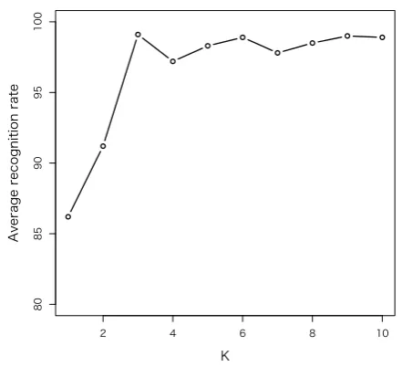
In this section, we discuss the abnormal gait detection. Okusa & Kamakura [14] only focused on K=3 case. In this paper, we apply K-NN classifier (K=1,...,10 cases), using the all estimated parameters, to perform normal/abnormal gait detect, and present results from an experiment involving 120 subjects (young person), and 60 subjects (elderly person). To evaluate our estimated parameters, we apply these parameters to leave-one-out cross-validation test.
Figure 15 is the average detection rate of K-NN classifier. x-axis and y-axis means K value and average detection rate respectively. Figure 15 shows estimated parameters are good feature values of the human gait. Most high performance case is K=3. However, K≥3 cases are high performance too like K=3 case. From the standpoint of calculation cost, we recommend to use K=3.
Table II is average detection rate of normal/abnormal gait
2 4 6 8 10
80
85
90
95
100
K
[image:7.595.56.274.74.271.2]Average recognition rate
Fig. 15. average recognition rate of K=1,...,10
(K=3). Table II shows our estimated parameters may be used for the normal/abnormal gait detection.
TABLE II
NORMAL/ABNORMAL GAIT AVERAGE DETECTION RATE(%)
Normal Gait Abnormal Gait
Normal Gait 98.2 1.8
Abnormal Gait 0 100
V. CONCLUSIONS
In this article, focusing on the human gait cycles, we consider the human gait modeling based on simple gait struc-ture. We estimate the parameters of the human gait cycles using the method of nonlinear least squares. We also show that estimated parameters may be used for the human gait analysis and abnormal gait detection. Experimental results verify that our model can estimate the various parameters and these parameters are good feature values of the human gait.
We plan to implement this scheme for the gait authentica-tion. The primary concern in gait authentication is realtime processing and fineness. In next phase, we focus on these problems.
REFERENCES
[1] C. Kirtley,Clinical Gait Analysis: Theory and Practice, 1e, 1st ed. Churchill Livingstone, 2006.
[2] J. Perry and J. Burnfield, Gait Analysis: Normal and Pathological Function. Slack Incorporated, 2010.
[3] M. W. Whittle, Gait Analysis: An Introduction. Butterworth-Heinemann, 1991.
[4] J. R. Gage, “Gait analysis for decision-making in cerebral palsy.”Bull. Hosp. Jt. Dis. Orthop. Inst., vol. 43, no. 2, pp. 147–163, 1982. [5] M. P. Kadaba, H. K. Ramakrishnan, and M. E. Wootten, “Measurement
of lower extremity kinematics during level walking.”J. Orthop. Res., vol. 8, no. 3, pp. 383–392, 1990.
[6] S. Borel, P. Schneider, and C. J. Newman, “Video analysis software increases the interrater reliability of video gait assessments in children with cerebral palsy,”Gait & posture, vol. 33, no. 4, pp. 727–729, 2011.
IAENG International Journal of Applied Mathematics, 43:1, IJAM_43_1_05
[7] S. Grunt, P. J. van Kampen, M. M. Krogt, M. A. Brehm, C. A. M. Doorenbosch, and J. G. Becher, “Reproducibility and validity of video screen measurements of gait in children with spastic cerebral palsy.”
Gait & posture, vol. 31, no. 4, pp. 489–494, 2010.
[8] R. A. Olshen, E. N. Biden, M. P. Wyatt, and D. H. Sutherland, “Gait analysis and the bootstrap,”Ann. Statist., pp. 1419–1440, 1989. [9] M. Soriano, A. Araullo, and C. Saloma, “Curve spreads−a biometric
from front-view gait video,”Pattern Recognit. Lett., vol. 25, no. 14, pp. 1595–1602, 2004.
[10] O. Barnich and M. V. Droogenbroeck, “Frontal-view gait recognition by intra-and inter-frame rectangle size distribution,”Pattern Recognit. Lett., vol. 30, pp. 893–901, 2009.
[11] T. K. M. Lee, M. Belkhatir, and P. A. Lee, “Fronto-normal gait incor-porating accurate practical looming compensation,”Pattern Recognit., 2008.
[12] K. Okusa, T. Kamakura, and H. Murakami, “A statistical registration of scales of moving objects with application to walking data. (in Japanese),”Bull. Jpn. Soc. Comput. Statist., vol. 23, no. 2, pp. 94– 111, 2011.
[13] K. Okusa and T. Kamakura, “A statistical registration of scale changing and moving objects with application to the human gait analysis. (in Japanese).”Bull. Jpn. Soc. Comput. Statist., vol. 24, no. 2, 2012. [14] ——, “Normal/Abnormal Gait Analysis based on the Statistical
Reg-istration and Modeling of the Frontal View Gait Data,”Lecture Notes in Engineering and Computer Science: Proceedings of The World Congress on Engineering and Computer Science 2012, WCECS 2012, 24–26 October, 2012, San Francisco, USA,, pp. 443–448.
[15] S. H. Collins, P. G. Adamczyk, and A. D. Kuo, “Dynamic arm swinging in human walking,”Proc. R. Soc. B: Biological Sci., vol. 276, no. 1673, pp. 3679–3688, 2009.
[16] K. Okusa and T. Kamakura, “Statistical registration and modeling of frontal view gait data with application to the human recognition.” in
Int’l. Conf. Comput. Statist. (COMPSTAT 2012), 2012, pp. 677–688. [17] H. Akaike, “Information theory and an extension of the maximum
likelihood principle,”Int’l. Symp. Inf. Theory, pp. 267–281, 1973. [18] N. Sugiura, “Further analysts of the data by Akaike’s information
criterion and the finite corrections,”Commun. Statist. - Theory and Methods, 1978.
[19] K. P. Burnham and D. R. Anderson,Model Selection and Multi-Model Inference: A Practical Information-Theoretic Approach. Springer, 2010.