Applications of a novel many component Lattice Boltzmann simulation

(1)

Applications of a novel many-component Lattice

Boltzmann simulation

DUPIN, Michael Maurice

Available from Sheffield Hallam University Research Archive (SHURA) at: http://shura.shu.ac.uk/10926/

This document is the author deposited version. You are advised to consult the publisher's version if you wish to cite from it.

Published version

DUPIN, Michael Maurice (2004). Applications of a novel many-component Lattice Boltzmann simulation. Doctoral, Sheffield Hallam University.

Copyright and re-use policy

(2)

Fines are charged at 50p per hout

(3)

ProQuest Number: 10694466

INFORMATION TO ALL USERS

The quality of this reproduction is dependent upon the quality of the copy submitted.

In the unlikely event that the author did not send a com plete manuscript and there are missing pages, these will be noted. Also, if material had to be removed,

a note will indicate the deletion.

uest

ProQuest 10694466

Published by ProQuest LLC(2017). Copyright of the Dissertation is held by the Author.

This work is protected against unauthorized copying under Title 17, United States C ode Microform Edition © ProQuest LLC.

ProQuest LLC.

789 East Eisenhower Parkway P.O. Box 1346

(4)

Applications of a novel

many-component Lattice

Boltzm ann simulation

Michael Maurice Dupin

July 2004

(5)

Abstract

There are many important systems which involve the flow of dense suspensions of deformable particles; blood is an example. However, the modeling of such materials represents a considerable challenge to established methods such as computational fluid dynamics (CFD). In this PhD project, work has been undertaken to extend the lattice Boltzmann method (LBM), and enable it to represent a large number of mu tually immiscible, deformable, droplets (separated by narrow interfaces). The new method imposes a relatively small computational overhead and has been validated against experimental observations. The work has also led to very promising develop ments in the simulation of micro-fluidic systems, allowing much quicker simulations than traditional CFD methods.

The principal target application of this project is the mesoscale modeling of blood flow, where the typical length is about 10 red blood cells’ diameters. We address in here the identified gap in models capable of modeling efficiently, explicitly, many deformable bodies within a surrounding incompressible fluid. We generalised, im proved, and extended an existing LBM model for binary fluids. Our N^>2 non coalescing fluids (droplets) are defined to represent the different deformable particles of the suspension. Their interactions with the walls as well as their deformability are controlled by local fluid-wall wetting and fluid-fluid surface tensions methods, which we have also been developed and validated.

(6)

access successfully the computationally non-trivial problems of binary fluid microfluidics.

Using our model, we also recover the expected behaviour of deformable and solid particle suspensions with respect to experimental observations on flow of solid and deformable spheres in pressure-driven straight pipe flow. In order to serve as cali bration, we measured the macroscopic effect of the droplets’ effective deformability against their microscopic properties (surface tension, internal viscosity).

(7)

Publications

This thesis contains work published in the following journals:

M. M. Dupin, I. H. Halliday and C. M. Care, Multi-component lattice Boltzmann equation for mesoscale blood flow, J. Phys. A, 36, pages 8517-8534, 2003.

M. M. Dupin, I. H. Halliday and C. M. Care, A lattice Boltzmann model of flow blunting, Phil. Trans. Roy. Soc. Lond. A, 362, pages 1755-1761, 2004.

(8)

Acknowledgments

The body of this work would not have been possible without the help and constant support of those around me, in England and back at home, in France. Firstly, I must thank my parents Andre and Micheline Dupin for always being there when I needed them, topping up my enthusiasm and providing inevitable financial support throughout my numerous years of study. I am also indebted to my twin brother, Patrick Dupin, for his friendship and for being very supportive, even though we did not have much chance to see each other during the whole of my PhD.

It has been a great pleasure to work with Ian Halliday for three years, and to have been his student for a year in final year of my BSc, here in Sheffield. He increased my confidence significantly and has always been there for me, when my life was not straightforward from time to time, just like my father or a good friend would have done. So, thank you very much Ian, I shall never forget. I would also like to thank Chris Care for his support and kindness.

I am infinitely indebted to Fabien Engel, with whom I started my University career back at home and with whom I came to Sheffield from Geispolsheim in France, in 2000. We discovered the joys of England together, this was certainly one of the best years of my life. Four years later, we are still very good friends. I would also like to thank David Michel (aka Cabrone) who has been a very good friend, colleague and house-mate.

(9)

(10)

(11)

Advanced studies

Sept.-Dee. 2001 Advanced technique in Mathematics, within the School of Science and Mathematics, Sheffield Hallam University, U.K.

11-13 Novem ber 2001 Fluent's Users Group Meeting, 2001, Hilton Hotel, Sheffield, U.K.

Jan-June 2002 Advanced Fluid Dynamics, within the School of Science and Math ematics, Sheffield Hallam University, U.K.

15-17 A pril 2002 Modelling Flow in Oil Reservoirs, BP Institute, Cambridge, UK.

5-9 A ugust 2002 11th International Conference on the Discrete Simulation of Fluid Dynamics, Shanghai, China.

2 July 2003 Presentation at the Conference on Physical, Mathematical and Nu merical Modelling of Blood Flow in Cardiovascular Disease, York, UK.

25-29 A ugust 2003 Presentation at the 12th International Conference on the Dis crete Simulation of Fluid Dynamics: from micro to meso to macro, Center for Advanced Mathematical Studies, Beirut, Lebanon.

17-19 Septem ber 2003 Presentation at the Computational Modelling in Medicine conference, Edinburgh, UK.

1 O ctober 2003 CCP5 Lattice-Boltzmann Workshop, Daresbury Laboratory, War rington, UK.

6-8 O ctober 2003 Fluent's Users Group Meeting 2003, Courtyard by Marriott Hotel, Rotherham, UK.

(12)

19-23 Jan u ary 2004 Towards a Predictive Biology, Isaac Newton Institute for Mathematical Sciences, Cambridge University, Cambridge, UK.

19 M arch 2004 Invited seminar, division of Engineering and applied sciences, Har vard University, Boston, Boston, Massachusetts, USA.

20 M arch 2004 Invited seminar, Steel Laboratory, Massachusetts General Hospital - Harvard Medical School, Boston, Massachusetts, USA.

29 M arch - 9 A pril 2004 Soft Condensed Matter Physics in Molecular and Cell

(13)

Introduction

Numerical techniques provide, very often, accurate answers to numerous problems that analytical theory cannot address. There exist an endless number of techniques, more or less general with many suited for a very precise application only, or for general configurations. Computational efficiency is always a decisive factor when choosing between techniques, since super-computing is still only available to a few research laboratories. Constant research is needed to ensure that the existing meth ods are being developed to the full extent of the capability of widely available hard ware and also to invent new method where existing models are inadequate.

In recent years, blood flow has been subjected to a high degree of interest by the scientific community, since it is believed that it is often responsible or a consequence of numerous pathologies and complications: from the turbulent heart and artery flow, to the micro-capillary retial flow, improper blood flow is often identified as responsible.

Better understanding of how blood flows and how biological cells interact is there fore needed to assist developing new drugs and surgical techniques. This thesis is concerned in tackling the very complex problem of suspension modeling, especially mesoscopic blood flow, where every biological cell has to be explicitly represented in the surrounding fluid.

(20)

meso-scopic modeling of deformable particles.

This is an acknowledged non-trivial problem, (and therefore highly rewardable). This thesis sets one of the first mile stone in LB’s application, by opening new research opportunities and capabilities.

Aims

The primary aim of this project had been to develop a technique capable of mod eling, explicitly, a large number of non-coalescing droplets in solution. As a prime application, the simulation of mesoscale blood flow was obvious, since it is subjected to a large interest in numerous configurations. Other current models can either rep resent a large number of solid particles in solution or a few deformable particles in solution (and that at high computational cost). There exists therefore, a great challenge for a model that would resolve explicitly and efficiently, a large number of deformable particles in solution.

The secondary aim of this project (which turned out to be as important as the latter) has been to improve the Gunstensen method in Lattice Boltzmann, which is subjected to significant micro-currents, generating a very noisy flow field and reduced stability of the simulations at low Reynolds number and Capillary number. Reducing significantly the micro-currents allowed the efficient simulation of binary fluid microfluidics devices, which grew into an obvious aim while developing and realising the potential and advantage of this method.

It turned out that reducing the micro-currents was necessary anyway, for an eventual simulation of mesoscale blood flow.

Thesis layout

(21)

con-sistent point of view to fluid dynamics. The link between fluid dynamics and Kinetic theory is made explicit. A second part consists of introducing and de scribing the construction the LBM. It describes in details the steps involved in the algorithm and how it is closely related to the previous Boltzmann Kinetic theory and to fluid dynamics. This chapter contains a literature review of the main, current numerical techniques for fluid dynamics.

C hapter 2: Specific background. This chapter beings by describing the link be tween a previous LB equation of motion, described in previous chapter, and that of the binary case and the main associated issue: the discontinuity of the equation of motion induced by an interface. It then describes, the general isation of Gunstensen’s LBM, described in the previous chapter. Each step is detailed and the explicit link to LBM is made explicit. Surface tension in the Gunstensen algorithm is then described, showing the original Gunstensen method and the more recent Lishchuk method, which provides a more accurate answer, introducing by the same token, the issue of micro-currents. This chap ter finishes by a discussion on stability issues in the binary LB model, mainly centered on the microcurrent issue (omnipresent in this thesis). This chap ter also describes a method to implement no-slip solid boundary conditions in LB simulations (moving or static) and a review on the different numerical interfacial methods, in CFD and LB.

C hapter 3: Novel m ethod to reduce th e m icro-current s. This chapter begins by reviewing the previously introduced micro-currents. It shows that these are not LB related issues only and that most numerical methods have a form of associated unwanted flow. It then describes and investigates their possible origin in the original Gunstensen surface tension method, in an ab — initio

(22)

C hapter 4: The N -com ponent algorithm . This chapter begins by reviewing the current models for the simulation of suspensions, in the blood flow appli cation especially. It demonstrates that current models are unable to simulate realistically and/or efficiently mesoscopic blood flow or deformable particle suspensions. It therefore introduces the main assumption of this thesis: the representation of biological cells as viscous, liquid, non-coalescent droplets in suspension. It then describes how to generalise the previously described Gun stensen LB algorithm to N 2 droplets. The generalisations of each step of the algorithm previously described in chapter 1, 2 and 3 are described in details. This chapter finishes by providing proofs of capability for our new model, related to the current application.

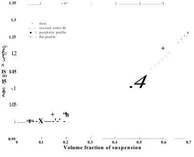
C hapter 5: Validation of the N -com ponent m ethod. Previous chapters had shown how to generalise and obtain a new technique for the simulation of the a large number of deformable particles, but only provided proofs of capability. This chapter consists, therefore, in a series of simulations validating the hy drodynamics of our N-component model against experimental observations. It shows that our new model recovers, correctly, some experimental observations of mesoscopic suspensions. It also provides a calibration of the solidity of the droplets in suspension with respect to their parameters (viscosity and surface tension).

(23)

Chapter 1

General Background: Classical

Fluid Dynamics

Introduction

(24)

1.1 Introduction to Fluid dynamics

It is unavoidable, within the context of this thesis, to describe the derivation of the equations of motion of a fluid (despite being very interesting by themselves). They are the equations that any computer model (including CFD or LBM) has to solve in order to be able to claim that the output post-processed pictures and extracted num bers have any physical meaning. It will be shown first that the macroscopic fluid motion can be derived without any reference to the detailed microscopic atomic structure, only by considering physical fundamentals (which is actually quite fortu nate, since it simplifies the task a lot: it would be rather complicated and expensive to consider the individual motion of each individual molecule involved!).

1.1.1 Different points of view

Different fluid flows have common properties. As an illustration, let’s consider the flow of the explosion of a supernova. It is believed that when a supernova explodes, a shock wave rushes towards the outer space, inducing a compression zone on its front and depression zone on its tail (standard shock wave). Before exploding, the star had a well defined radial structure, with heavy elements concentrated within its inner layers and lighter elements towards the outside. The negative pressure gradient is directed from the outside to the inside (due to the shock wave), accelerating heavier matter towards lighter matter. It can be shown that acceleration due to a pressure gradient is equivalent to the acceleration due to a force such as gravity, acting towards the centre of the star [209], [63]. This leads to the rather surprising result that the flow of the explosion of a super-nova can be correctly described by the flow of the Rayleigh-Taylor instability (or density fingering), where a heavy fluid sits on the top of a lighter one and both are subjected to the same gravitational field. This is very useful to understand the dynamics of these explosions, since the Rayleigh-Taylor instability is much easier to investigate (analytically, numerically and obviously experimentally).

(25)

commonly used way of imposing numerically a pressure difference in the simulation of a pipe for example, at low Reynolds number, is to set an explicit body force (like gravity) to drive the flow.

1.1.2 Fluid macroscopic continuum m otion

This section follows essentially Anderson’s second chapter ([2]) and concentrates on setting the general fluid flow equations (that any model must recover), namely the NSE (including the continuity equation).

In obtaining these basic equations of fluid motion, one always begin with the fol lowing fundamental principles from the laws of physics:

• Mass is conserved.

• F = m a (Newton’s second law).

• Energy is conserved.

Each of these fundamental principle will be the starting point of an analysis leading to a fluid motion equation.

The continuity equation

The continuity equation is the fluid dynamics analogue of the chemical law by the French Chemist Lavoisier: ‘nothing is created, nothing disappears’ applied to a set volume of fluid. A control volume, V, represents a finite volume of fluid, where matter is counted. It is bounded by its control surface. First, these control volume and surface are considered to move with the flow, expanding or shrinking along any flow velocity streamline. The mass conservation principle implies that the total mass in this control volume has to be constant throughout time, in equation:

(26)

observer is going along or ‘advecting’ with the particles). Despite being the most fundamental form, the ‘material derivative’ in equation 1.1 is not easily obtained or very useful in any analysis, and is very often replaced by an expression containing its subsequent set of partial differential operators. They can be obtained by fixing the coordinate of the control volume (the observer now looks at the fluid from above, and is still unable to distinguish any atomic structure) which splits the total derivative

Dt into partial derivatives. For quantities depending on time and position only (such as velocity), Dt becomes (from e.g. Batchelor [6]):

A = ft + V - v . (1.2)

Dt is also called the substantial derivative, which is physically the rate of change following a moving fluid element, dt is called the local derivative, which physically represents the time rate of change at a fixed point and V • v is the convective

derivative, which is physically the time rate of change due to the movement of the fluid element from one location to another in the flow, taking spatial difference into account (from e.g. Anderson [2]). The continuity equation (1.1) becomes:

J J j [c>,P + v •(pv)]dK=°. (1.3)

This form is designated as the integral conservation.

The integral in equation 1.3 would make it necessary to make explicit the control vol ume V, which could be a drawback in the following derivation. This can be avoided by making the control volume infinitesimally small, and equation 1.3 becomes:

dtp + V - (pu) =0. (1.4)

This latter form is the differential conservation form of the continuity equation, for compressible fluids. Note that u denotes the macroscopic velocity and is defined as follow:

U =

III

VC^'

(27)

The last form of the continuity (equation 1.4) is said to be least fundamental since it does not allow for the presence of discontinuities, for it assumes the flow properties to be differentiable, hence continuous. It is therefore not surprising that it leads to significant errors when investigating real flow discontinuities such as shock waves (very local zones of high and low pressures). However, this latter form is just as valid for the type of flow involved in this thesis (incompressible, low Reynolds number). We will consider incompressible fluid only, in which the time derivative the continuity equation vanishes (by definition, no spatial or temporal gradients in density), and from equation 1.4:

V - ( p u ) = 0 . (1.6)

This is to be the equation referred to as the continuity equation throughout this text, even though the three forms of the continuity equation (equations 1.1, 1.3 and 1.4) all represent the same behaviour (conservation of mass), applied under different circumstances.

M om entum equation

In continuing to derive the fluid motion equations, one needs next to consider the second listed law of physics: Newton’s second law. This section considers the forces moving and deforming the control volume V considered in the previous section. The control volume experiences two types of forces: body forces (represented by A hereafter), which act on the volumetric mass of the fluid element (gravity, electric and magnetic forces) and surface forces, which act on the surface of the fluid element [2]. The surface forces are from two sources only: (a) the pressure distribution acting on the surface by the static surrounding fluid (represented by P ) and (b) the shear and normal stresses acting on the surface by the outside fluid tugging or pushing

on the surface by means of friction (represented by cra/j). Within these frames, the total net force per unit volume acting on the moving fluid element in the a direction can be written as:

(28)

where aap represents the stresses exerted on the fluid element by the surrounding fluid and relates to its time rate of change of its deformation. The diagonal and non-diagonal components of oap have different physical meanings, yielding to its explicit separation: the diagonal terms are written cr" and the non-diagonal terms are written as a'a/3

< < y Uxz \

< r ° y_// ° y z_ / (1.8)

< y ° z

)

The viscous shear tensor (or shear stress tensor), denoted above by a'a/3 (a ^ p)

relates to the time rate of change of the shearing deformation of the fluid element, responsible for the strains of the elements of the fluid. The normal stress tensor, on the other hand, denoted by <r" relates to the time rate of change of volume of the fluid element (pressure). It must be understood as mechanical pressure, defined in terms of the mechanical stresses that act on an element of fluid. As a result of equation 1.7, both shear and normal stresses depend on velocity gradients of the flow and the rest of this section consists of describing the relation between cra/3 and

OaUp.

The normal stress tensor

Let’s consider the normal stress tensor first. Pascal’s theorem states that stress in a fluid in mechanical equilibrium (no flow) is a scalar quantity (unaffected by changes in the reference frame), completely described by an invariant isotropic pressure P

(29)

where P is the thermodynamic pressure. Therefore, in a stationary fluid, the ther modynamic fluid pressure is defined as the average value of the three components of normal stress, i.e.

where 5ap is the Kronecker function.

Stokes, in 1845, obtained that the three normal stresses are unequal in a moving incompressible fluid and defined as [2]:

<7" = P - fi2daua - C V • u ,

where fj, is the molecular viscosity coefficient and £ is the second or bulk viscosity. The term associated to £ corresponds to the changes in the volume of the fluid due to compression effects (note that V -u is the left hand side of the continuity equation 1.4) and as a consequence, for incompressible fluids this term vanishes. £ appears only in measurements of attenuation of sound- the propagation of sound in any fluid (including one which is incompressible) is necessarily accompanied by compressive effects (otherwise the speed of sound would be infinite) [81]. In the case of ordinary fluids, measurements lead to very small value of f (or big values of the speed of sound). For incompressible fluids:

o"a = P - 2fidaua . (1.9)

Note that the repeated subscript here is not a sum and that | cr" is still the thermodynamic pressure P (through the continuity equation for incompressible flu ids V • u = 0). Even with moving fluids, the differences between ax, cry and oz are most often found to be small and they are ignored for most practical purposes [208]. Viscoelastic fluids however are characterised by a significant direction dependance of cr" - that is, there are important differences between the normal stresses (i.e.

< ) ■

The shear stress tensor

(30)

i.e. velocity gradients. These fluids are therefore called Newtonian fluids and the non diagonal of the stress tensor is written as:

o 'o tP ~ f1 2<S'a/3) ( 1 - 1 0 )

where Sap is the strain rate tensor defined as follow:

Sa/3 = ^ {daUp + 8pUa) . (1.11)

Recalling equation 1.7 giving the net force the fluid element is subjected to, together with the definition of the shear stress tensor aQp (equations 1.8, 1.9 and 1.10), leads to the following momentum evolution equation of the velocities:

pD tua = PQ = pdtua + p(u • V) ua = —dp(jap + p A a ,

and after rearrangement, we obtain the momentum equation:

p dtuQ + p (updp) ua = - d aP + p dpSQp + p A a .

Sap relates to the dissipation in the tangential stresses due to the relative motion of the various layers of fluids (p is the molecular viscosity coefficient). The shear viscosity of a fluid is therefore the ratio between the rate of strain and the shear:

Strain

' ■ a S - ( M 2 >

and represents the dissipation of local stresses into the fluid. It can be understood as the molecular friction: a non viscous fluid would have its molecules sliding easily next to each other while the molecules of a highly viscous fluid would exchange much more momentum through collision. Accordingly, the density of the fluid obviously plays an important role in the rate of diffusion of momentum and needs to be taken into account for the quantification of the rate of dissipation of stresses. Therefore, the quantity i/ defined by:

v = ^ (1.13)

P

is called the Kinematic viscosity or simply viscosity, where p is the shear viscosity defined by equation 1.12 and p is the density of the fluid.

(31)

one example as is discussed in chapter 4. If the stress increases faster than the rate of strain (viscosity increasing with the rate of strain), the fluid is said to be shear-thickening (wet sand for example), and shear-thinning vice-versa (paint, blood, or ink). Other examples of complex behaviours are Bingham fluids (no flow is observed until a critical value of the stress: clayey muds, toothpastes and fresh cement are few examples), or thixotropic fluids (effective viscosity decreasing with time) such as ketchup or drilling muds.

Energy equation

Following similar steps as previously for the second Newton’s law, which lead to the momentum equation, the energy conservation principle leads to the derivation of the energy equation for the fluid. One first states that since energy is conserved: the rate of change of energy inside a fluid element has to be equal to the sum of the net flux of heat into the element and the rate of work done on the fluid element due to body and surface forces. One then obtains an equation which allows the study of temperature diffusion or combustion. This energy equation won’t be discussed further since the LB method used in this thesis does not allow any temperature gradients. Moreover, the energy equation does not bring any more information on the flow of an isothermal fluid, the previously described NSE and continuity are sufficient to close the description.

Sum m ary: E quation of m otion of the flow of interest

The flow of incompressible (dtp = 0) non-viscoelastic (isotropic pressure) newto-nian (linear relation between strain and stress, or constant viscosity) fluids can be described by two equations: continuity and momentum equations. The continuity equation reads as follows:

V • u = 0, (1.14)

which ensures that the fluid is incompressible. The momentum equation dictates the effects of external forces and the dissipation of stresses:

(32)

The momentum equation is called the Navier-Stokes equation, but it is widely under stood, however, that the term Navier-Stokes equations encompasses the continuity, Navier-Stokes and Energy equation (not described here).

For completeness, it should be noted that Euler had derived the continuity and mo mentum equation for inviscid flow (null viscosity) but had not derived the energy equation since the science of thermodynamics did not exist at the time. Therefore, a fluid with no dissipation due to viscous stress is identified as a Eulerian fluid, obeying the Euler equations (NSE with /i — 0):

VP

ftu + (u -V )u = F - - ^ - . (1.16)

1.1.3 Boundary conditions for fluid flow

G eneral rem arks

The NavierStokes equations can take on different forms depending on flow regime:

• Incompressible, steady: Elliptic,

• Incompressible, unsteady: Parabolic,

• Compressible, steady: Elliptic/Hyperbolic,

• Compressible, unsteady: Parabolic/Hyperbolic.

Different numerical methods will succeed in different regimes and therefore different formulations are used to handle compressible and incompressible flow cases.

Mathematical principles on PDEs states that the NSEs should have u defined over all the boundaries of the flow domain. Therefore, boundaries can’t be overlooked and should be subjected to great care. The two main types of boundaries that will be considered are walls and other non-miscible fluid.

B oundary conditions: solid walls

(33)

between the tangential velocity of the fluid and the boundary would lead to infinit energy dissipation at the surface as a result of the non-null viscosity and therefore cannot be allowed. This leads to the non-slip boundary condition:

U fluid ' ^ = U solid ’ ^ (1.17)

Note that this condition is valid for a solid wall as well as for deformable (moving) walls. Cavitation happens when nearby layers of fluid cannot keep up with the layer of fluid immediately next to the very fast moving wall, due to too small a viscosity, leaving an increasing space between them, leading to low pressure and the formation of bubbles (very often accelerated to supersonic velocities by the very important pressure gradient). On the other hand, in the case of non-moving walls, fluid immediately next to it should have zero velocity.

Boundary conditions: fluid interface

The other type of boundary is the an interface between two fluids. Fluid interfaces can be considered at two levels: the macroscopic (continuum) level and the micro scopic (discrete) level. This section concentrates on continuum fluid dynamics and will therefore consider the continuum representation of fluid boundaries. We refer to Rowlinson and Widom [171] for microscopic information about interface structure. In the case of an interface between two fluids ( (1) and (2) ), the tangential stresses should be continuous through the interface (to avoid any cavitation of the two fluids):

where na and ta are the normal and tangential unit vector of the interface. It can be understood as the necessity for the interface to have no structure and therefore cannot be the host of any discontinuity (at least from a continuum point of view). Therefore, the condition that the tangential stresses should be continuous leads immediately to the condition (after equation 1.9):

V i d y U ^ = /j,2 d y U ^ ,

(34)

interface of the two fluids. This surface tension if the consequence of the difference of affinity and density of the two fluids in contact. The standard condition on the normal stress at the fluid interface boundary is given by ([116]):

(i) (2) / 1 , 1 \

nP ~ nP = 712 \ R 1 + 'F2) Ua’

As seen previously, normal stresses are closely related to pressure. The normal stress step of the interface corresponds macroscopically to a pressure step from the inside to the outside of the droplet, as defined by the Young-Laplace law:

A P = Pa — P2 = 7 l2 Q - + Y ) (1.18)

where 712 is the surface tension coefficient between fluid 1 and fluid 2, and R\ and

R2 are the local principal radii of curvature. The surface tension parameter is most often positive, indicating that the pressure is higher on the concave side of the interface.

Multi-component (>2) fluid interface

The same approach is taken in the case of an interface between N fluids: a line of contact is subjected to the tensions of the N different surfaces and, since it is without mass (by definition), the vector resultant of the N tensions must have zero component in any direction in which it is free to move. When one of the N media is a solid, the local surface of which will normally be a plane, the line of contact is free to move only in one direction parallel to the solid surface. The following single scalar condition for equilibrium is then given by (in the case of three media, where media 1 is the wall, and 1 and 2 are fluids) by:

712 = 731 + 723 cos6c (1.19)

which determines and defines the angle of contact 9C (see figure 1.1).

1.2 Classical Fluid Dynamics modeling techniques

1.2.1 Euler vs Lagrange

(35)

Fluid 1

BC 'AB

Fluid 2

AC

Fluid 3

Fluid 2

AB _{Fluid 3}

'AW BW

wall

Figure 1.1: Surface tension geometry in the case of three components.

mean free path of a molecule [125]. This is to ensure good statistics of the different quantities within the volume of fluid (particle) and consequently their averages and evolution. When this applies (for most gas problems at normal pressure and for most liquid problems), the fluid can be treated as a continuous medium and two distinct alternatives of fluid specification are possible, differing in their reference to the fluid. The first one, the Lagrangian description, considers a fixed volume of fluid V given at a time reference (t = 0 generally) advecting with the flow. The flow observables are defined as functions of time and of the choice of material element of fluid, and describe the dynamical history of this selected fluid element (contained in the moving volume V). Useful in certain special contexts, it leads however to rather cumbersome analysis and is at a disadvantage in not giving directly spatial gradients in the fluid ([6]). That is why a rather less complicated approach is used: the Eulerian approach. Here the velocities considered are at a fixed point. At each instant of time, the velocity field describes the velocity of different fluid particles (of volume V). Methods describing explicitly each molecule are qualified as Lagrangian while any grid-based approach is therefore qualified as Eulerian. LB is Eulerian.

CFD techniques

(36)

will then be described, showing its essential difference: it is restricted and designed to solve the NSE (with additional terms as well such as gravity, surface tension, and other effects if necessary).

Finite difference

The whole idea of discretisation is to replace the (infinitesimal) partial derivatives of the NSE with a suitable (finite) differences quotient (definition of a derivative), i.e. a finite difference. This implies a discretisation of the simulational space. Most common finite-difference representations of derivates are based on the Taylor series expansions, where the zeroth order is a first guess (not really good), the first order adds information to capture the slope of the curve and the second order its curvature. It can be shown that partial derivatives can be written as:

& ( « ) = Ui+1’f f x UiJ + O(A 2 0 = 1 2 A :r + ° (A x )2 ’

dt(u) = Ui'^~x Ui'{ + 0(Aa) = — + 0(A s)2 ,

where Uij is the quantity of interest, i is the spacial index and j is the time index. It can be noticed immediately that the accuracy of the solution will depend greatly on the chosen accuracy of the finite difference.

finite volume methods

Finite volume methods do not differ much from the finite-difference technique in that they also involve a discretisation, but now of the integral form of the evolution equation this time. For example, the

equation:-*

III

pdV + J J p udS — 0,

is the integral form of the continuity equation (where S is the control surface bound ing V). Replacing these integrals by finite volumes (which is what an integral rep resents) enables integral equations to be solved.

(37)

1.3 Kinetic Theory: from Atom istic Dynamics to

Thermodynamics

The last section derived the NSE describing the macroscopic fluid flow that fluid dynamics solvers (like LBM) have to recover, it is however necessary to start from the atomistic level (microscopic) to derive the LBM which, as we will see, recovers the NSE to a very good accuracy. This first part follows essentially S. Succi’s ap proach towards LB, from his book The lattice Boltzmann equation. [190]. Additional information has been taken from the on line lecture notes by J. R. Graham’s from Berkeley University on Astrophysical Gas Dynamics [77], from Statistical Physics and the Atomic Theory of Matter, from Boyle and Newton to Landau and Onsager

by S. G. Brush [21], and from the unavoidable text book by S. Chapman and T. Cowling [28] (The Mathematical Theory of Non-Uniform Gases).

1.3.1 Atom istic dynamics

Boltzmann’s original concern was to derive the second law of thermodynamics for continuum physics from principles of classical mechanics, and gather more insight on the apparent contradiction on irreversibility of continuum mater (second law of thermodynamics) and reversibility of discrete matter (classical Newtonian mechan ics). Through this process, in 1868, he derived a law of velocity distribution for a gas at equilibrium, with an external force field such as gravity present (thus expanding the previous Maxwell’s law) [21]. This had been one of the first milestone of kinetic theory, which lead to the description of the motion of a fluid four years latter (still by Boltzmann). In that sense, kinetic theory describes the motion of a fluid by considering a large number of molecules rather than each of their individual motion.

1.3.2 Boltzm ann approach

Momentum distribution function

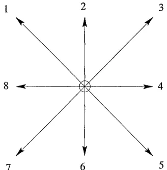
First, the following key quantity has to be defined: what is the number of molecules in a volume (Ax)3 with velocities in the range v and v ± A v?

(38)

indeed very powerful since the quantity / does not have to be quantified, precisely its evolution and statistics are enough to derive the laws of fluid motion. Making Ax and Av infinitesimal, the number / becomes a probability depending on position x and velocity v. In fact, this infinitesimal point of view is from the continuum level, where the number of molecules considered in V is large and V itself is very small compared to the macroscopic length scale (which crosses the definition of fluid’s

particle mentioned previously). This distribution / is the pivotal object in kinetic

theory, and will be omnipresent in this thesis.

Macroscopic observables from the momentum distribution function

Integrating the distribution / over v won’t necessarily add up to unity, since / is derived from a non-normalised number of molecules, and leads to:

J /(x ,v )d v = Nmoi(x) ,

where Nmoi(x) is the total number of molecules at V and x. In addition, since / relies to a constant finite volume of fluid (taken to be unity), we have:

m J f (x, v ) dv — p (x ), (1.20)

where m is the mass of the fluid particle and p(x) is the fluid weight at x, in the volume V: its density. The distribution’s total momentum and total energy are simply the sum (or integral) of all the associated momentum and energy of each molecule. They can be computed by ‘moments’ of /:

m

f

/(x, v) va dv = p(x) ua(x) (1.21)

f(x ,v )v 2/2dv = p(x)e(x) (1.22)

(39)

one time, it could compute their positions and motions at any other time as well as the macroscopic properties of that gas. Modern quantum physics, however, opposes such an idea through the Heisenberg uncertainty principle, that the accuracy on the position of a quantum particle (such as a gas molecule) and the accuracy on its speed are balanced (there would be no point in wanting to find the precise trajectory of a molecule if its position or velocity were to be subjected to a great uncertainty). Quantum restrictions don’t allow a direct bridge to continuum physics, but kinetic theory does!

1.3.3 The Boltzm ann equation

In 1872, Boltzmann presented, in a long paper, the evolution equation of the pre vious quantity / derived from atomistic interaction, which became known as the Boltzmann Equation (BE). It is important to realise the apparent contradiction of the BE: it represents the non-stochastic evolution of an unquantified quantity!

Exact evolution

The first step towards the BE is to find the rate of change in time of /. As men tioned previously, / represents a large number of molecules rather than a single particle, and therefore its evolution cannot be represented by a simple time deriva tive (recall the Eulerian approach). The partial derivative with respect to time d/dt

represents the rate of change of a quantity at a point which is fixed in space and which is occupied by a succession of different fluid particles in turn. The quantity / represents a large number of particles on the move, on the other hand, and there fore these particles occupy a succession of different points (recall the Lagrangian approach). The answer to this paradox is readily found by the Taylor expansion, keeping the first order terms [77]:

^ d f , d f d f d f

Df = -£Tdt+ i + - 4 v 2 + -± -v3 .

u t OXi UX2 OX3

We will use the following symbol convention:

(40)

Following the fluid, the rate of change (or total change during dt) of the quantity / subjected to an external force F can be re-written as:

/(x + c dt,c + F dt, t + dt) dx dc dt —/(x, c, t) dx dc dt = £!(/) dx dc d t,

where fi(/) is the collision operator since Dtf is also equal to the rate of change of the particles undergoing collisions. Letting dt —> 0 gives the BE [28]:

D tf = dtf + (ua -da) f + Fa - dca f = f t( /) . (1.23)

First assumption

The simplest case is to consider the one body distribution f\ (note that in this chapter, unless otherwise stated, the subscript C on fc represents the number of bodies of the distribution), and equation 1.23 reads as follow:

Dtfi = dtfi -f- (ua • da) fi + Fa • dca fi = C2 , (1-24)

where C2 is the binary collision operator (note that C\ is absurd) and represents the effect of intermolecular (two-body) collisions taking molecules in/out the streaming trajectory (C2 = Dtfi). Equation 1.24 is the beginning of the so called BBGKY hierarchy, after Bogoliubov, Born, Green, Kirkwood and Yvon [12] where the dy namic equation for f 2 depends on the three-body distribution function / 3 which in turn depends on / 4 and so on down an endless hierarchy [190].

To close this hierarchy, Boltzmann made few stringent assumptions on the na ture of the physical system that was considered: a dilute gas of point-like and

structureless molecules was assumed. This assumption has the consequence (un fortunately) of erasing any dependance of the dynamics upon the detailed chemistry of the molecules. However, within this picture, the collision operator of equation 1.24 becomes the (self sufficient) integro-differential function:

C2 = j[f2 (v ,v v,2) - f 2{vi,V2)\G{vu V2,v,1,v'2)d3v , (1.25)

where the function G depends on the nature of the forces between the molecules, {^1, V2} are the pre-collisions velocities of the colliding particles (remember that C2

(41)

Second assum ption

At this point, Boltzmann made another assumption: there is no statistical corre lation between the velocities of two molecules before they collide (and therefore after collisions). In other words, they interact via short-range two-body potentials. Elementary statistics reminds us that the probability of two uncorrelated events is simply the product of their respective probabilities, which leads to the famous Boltzmann closure assumption, molecular chaos or Stosszahlansatz [11]:

f2{v'1,v'2) = /i(ui)/i(u2).

This is the main assumption in his theory and is still the subject of active dis cussions because even-though this assumption is reasonable for dilute gas where molecules spend most of their life traveling alone and being absolutely unaware of their surroundings, it is certainly not so true for liquids. It should also be noted that, even-though it is reasonable to assume no correlation between the molecules before they have ever collided (at the beginning of time say), this lack of correlation for a particle is immediately lost after its first collision, by virtue of mass, momentum and energy conservation.

Summarising, the BE takes the following form ([125]):

(0f + u -V + F -d p)/i = J [fi(v[)fi{v2) - /i(v i)/i(v 2)] G(v1,v2iv[1v2)d3v .

The beauty of this equation is that it links atomistic and continuum behaviour. The left hand side is the faithful microscopic reversible Newtonian single-particle dynamics while the right hand side describes continuum intermolecular interactions which, we will see in next section, is irreversible. Additional terms can be added to take account of gradient of temperature and fluid velocity, and are known as the

Boltzmann’s transport equation. Boltzmann then showed that collisions always push the distribution / towards the so called Maxwell-Boltzmann equilibrium distribution function (note that Maxwell had first given the definition of this distribution [28] by deriving the equilibrium velocity distribution of gases, but without external force).

Dynam ical evolution of any fluid velocity distribution: th e H -theorem

(42)

showed that the following quantity:

H = / / log(f) dv

was always decreasing (a formal derivation can be found in [164] or [125] for exam ple):

DtH < 0.

In other words, this (H-) theorem states that a uniform gas with a random distri bution of velocity will decrease monotonically to an equilibrium state through the effect of collisions. That is, only when fi (uj) = fi{vi)fi(v2) (hence DtH = 0),

which introduces the notion of local equilibrium: when the distribution remains un changed under the effect of collision (hence time). It should be emphasised that the H-theorem is not in general the same as the principle of monotonic increase of entropy (second law of thermodynamics), in that H is only defined for a uniform gas (see previous Boltzmann’s assumptions) while the entropy can be defined for com plex systems. Moreover, H is defined for any distribution while entropy is only for system in thermodynamic equilibrium. Therefore, only the special case of a dilute gas in thermodynamic equilibrium can H and entropy be defined at the same time. Under these circumstances, the entropy is related to H by S = — IcbH + K where

S is the entropy of the system, ks is the Boltzmann constant and K is a constant [125],

Boltzmann further showed that the collisions are pushing the distribution / towards the equilibrium Maxwell distribution. The iJ-theorem is equivalent to the generali sation to a dilute gas at non-equilibrium to the statement that the entropy always increases or remains constant (2nd law of thermodynamics) [21].

(43)

both ultimately to Clausius’ idea of Heat Death, namely the universe as a whole evolves in a unique way towards a state of maximum entropy (and minimum H)

where all energy is diffused uniformly through space at a temperature very close to absolute zero, so that no mechanical work can be done and life cannot exist. This rather disturbing idea goes along side the idea of unavoidable and unidirectional decay of matter into lead. For further readings, see the section irreversibility of D. Levermore’s website from the University of Maryland [123].

The next section will concentrate on defining this equilibrium distribution function

introduced by the iT-theorem.

1.3.4 Relaxation to local equilibrium

It is important at this point to distinguish between two different equilibria: the

‘state’ or (macroscopic’ or ‘global’ equilibrium and the ‘thermodynamical’ or ‘mi croscopic’ or ‘local’ equilibrium. The main difference lies in the scale at which they may be represented. Global equilibrium is reached when the macroscopic properties of a system’s constituents are not observed to change as further time elapses (density, pressure, temperature, magnetisation, etc) while thermal equilibrium is compatible with rapid spatial variations in the state of the system at the microscopic level of its constituent molecules. Local equilibrium is defined mathematically as a local distribution function / e, such that gain and loss to the microscopic system are in exact balance [125], so that from equation 1.24:

C2( f e, f e) = 0, (1.26)

where the subscript 'd denotes 'equilibrium1 hereafter. After equation 1.26, this leads to:

fi(v[) fi(v'2) = fi(vi) /i(v2) • (1.27)

Following Liboff [125], the logarithm of equation 1.27 gives:

ln(M vi)) + M / i M ) = ln( M vi)) + M / i M ) • (1-28)

(44)

addition, at thermodynamic equilibrium, ln (f) must be a linear combination of the three collision invariants defined previously (namely mass, momentum and energy) ([28]):

ln (fe) = A + Ba va + C u2/2,

where A, Ba, C are five Lagrangian multipliers defined solely by the macroscopic observables (equation 1.20, 1.21, and 1.22). Elementary quadrature of Gaussian integrals delivers the celebrated Maxwell-Boltzmann equilibrium distribution [190], giving the number of molecules (or probability) with velocity v with respect to their local density p at a temperature T. In D spatial dimensions:

/ e(v, p, T) = p (2 7T , (1.29)

where c is the so-called peculiar velocity

c = v — u , (1.30)

and

[ K ^ f

v t = \ --- , V m

is the thermal speed associated with the fluid temperature T. It is interesting to note that f e only depends on the fluid’s local macroscopic observables, and is independent of the local neighbouring, chemistry or external fields (it can therefore be greatly different from time to time and from a point in space to another). This infers for this function a notion of absoluteness, which can be viewed as a weakness: it is legitimate to question its applicability and validity when considering the assumptions made to obtain this equilibrium distribution, and whether what it represents alongside its dynamics are representative of a real fluid. One could even argue that Boltzmann did everything he could possibly do to get to this result, which shows the limits of this distribution function and demonstrates its paradox: even though it claims to be absolute, it lacks applicability to any real fluid.

(45)

1.4 From kinetic theory to fluid dynamics

1.4.1 The Boltzm ann transport equation

General statements cannot be easily extracted from the BE apart from the

H-theorem. A more fruitful approach considers its moments: the one associated with the mass and momentum in particular. Multiplying the BE by some func tion Q(x,v, t) and integrating over all velocities, gives after some algebra:

dt J f i Q d v -J f i d t Qdv + da J Q fcva dv - J A vada Q dv

+ J FadcafiQ d v = J QD t f 2dv. (1.31)

Equation 1.31 is the transport equation, and tells us how the volume density f fiQ d v

of any quantity that is conserved in binary collisions evolves with time. For a such a quantity Q, the second term f f \ d t Q dv and the collision integral J Q Dtf2 dv

vanish [77]. .

First, setting Q to m (the particle’s mass), the volume density f fiQ gives p and any of gradient in Q (spatial or temporal) vanish (because the fluid is considered as incompressible). Therefore, equation 1.31 yields the mass conservation equation seen previously in this chapter (continuity equation 1.6):

dtP + da{pua) = 0.

Second, setting Q to m u a (the particle’s momentum), the volume density f fiQ d v

gives pua and (after some algebra), f vafd a m updv gives da(P5ap — cr^), where

a'ap is the dissipative term of the momentum stress tensor (see equations 1.8 and 1.10). Therefore, equation 1.31 yields also the momentum conservation equation:

dt(pup) + da(pua up + PSap - <j'ap) +pFp = 0.

This equation can be recognised as the NSE (equation 1.15) and verifies that the ('microscopic) BE recovers the (macroscopic) NSE introduced in previously.

(46)

1.4.2 Bhatnagar-G ross-K rook model equation

Since we have defined a (universal) equilibrium distribution function, any distribu tion can be written in the form:

/(x , v, t) = / e(x, v, t) + g(x, v, t)

where f e is the Maxwellian distribution function (see equation 1.29) and g describes any departure from it. With this definition, in 1954, Bhatnagar, Gross and Krook

where vc is the collision rate associated with the collision time rc = l/^ c- This is the so-called BGK collision operator. Equation 1.33 is named the BGK equation and is much easier to solve than the integro-partial differential equation that is the BE, and most of all, without spoiling the basic physics. Since isc can be regarded as independent of /, the BGK equation is linear in /. This allows much easier com putation of the transport coefficients and provides a great advantage in subsequent computer models (like LBM) [190].

1.4.3 The Chapman-Enskog procedure

Since the BGK equation provides a simple alternative to the BE, it is interesting to investigate the consequence of the simple collision operator structure on its moments. To do so, a characteristic small parameter needs first to be defined. It is usually taken to be the Knudsen number (see J. R. Graham [77] for a justification of this choice), namely the ratio between the molecular mean free path and the shortest scale at which macroscopic variations can be appreciated (note that the bridge between micro and macro becomes explicit here):

[9] re-wrote the BE (equation 1.23) in terms of equilibrium and non-equilibrium parts:

(1.32)

therefore,

(47)

parameter of both dependent /(x , v, t) and independent space-time (x, t) variables (see [125], [28] for a detailed derivation of this expansion). First, the momentum densities are separated between equilibrium and non-equilibrium ( / ^ ) parts:

/ = / (0) + e /(1).

Note that the major difference between g defined in the BGK equation and here is that is assumed 0(1) (the smallness of the non-equilibrium part is carried by the pre-factor e) while g carried the smallness and is therefore much smaller than It should also be understood that defined as above contains implicitly a whole series of terms: / = £n / ^ (where each f n is 0(1)).

Second, time and space are expanded up to the second order:

{

x = e_1X i,

t « e-1 ti + e~2t2 ,

and the differential operators likewise:

{ dx ~ £ dXl,

dt ~ edt l + e2 dt2, hence the streaming operator becomes:

I

Dt ^ e dti + e dt2 + e uadai + -e 2 ua up dai dPl.

This analysis will be restricted to the second order of the time expansion for reasons that are explained latter. In this analysis, x \ and represent the linear (sound wave) fast regime while t2 represent the long-term (slow) dynamics. This segregation between equilibrium term (fast) and non equilibrium term (slow) is explicit in the moments of the subsequent equations. The zeroth order term of the distributions is the local Maxwell-Boltzmann distribution function defined in equation 1.29. Similarly as in section 1.4.1, we integrate the BE over v and take its zeroth and first moments. The first order solutions are found by considering 0(e) in the integrated BE and give (for the zeroth and first order momentum respectively):

(48)

dtipua + dp, (puaup + PSap) = 0,

where P = p T is the fluid pressure. These equations are recognised to yield the Euler equations of inviscid flows (equation 1.16). However, although this represents a dynamical evolution of a fluid, the fluid’s viscosity is missing in the equation: the distribution of the fluid had been assumed to be the local Maxwellian distribution at all points at all times. Transport phenomena occur when there are large gradients of temperature or velocity, and this should be taken into account in the evolution of f (not only / ^ ) .

It is therefore important to investigate the non-equilibrium moments. The second order solutions are found by considering 0(e2) in the integrated BE and read as follow:

dt2p = 0,

dt2pua + d0l rn J ( / (1) + d7v7 / (0)) ua updv = 0.

In fact, by splitting / into equilibrium ( / ^ ) and non-equilibrium ( / ^ ) components, it can be shown that the two integrals represent the equilibrium and non-equilibrium components of the momentum flux tensor Pap defined as follows:

Pap = m J f va vp d v.

Respectively (for an incompressible fluid):

I PaP — 'Pap T Tap,

< Tap = m f / (0> VQ Vp = pUa Up + P8ap ,

rap = m f f {1)VaVp = 2fi Sap.

It is important to notice here that the dissipative term of the momentum flux tensor

(rap) is equal to the viscous stress tensor cr^ (equation 1.10) which can therefore be computed purely locally. It provides a great reduction in its computation in the subsequent method (LBM).

Finally, joining the non-equilibrium and equilibrium parts of the zeroth and first moment of the BE order by order gives the NSE.

(49)

fluid behaviour, despite the assumptions necessary to get to this result. It therefore demonstrates the fact that the NSE contain, implicitly, the same assumptions as Boltzmann’s (hidden in its large time and length scale). It can also appear rather surprising that the second order in the truncation of the Knudsen number e does re cover the full NSE, but it is fortunate on the other hand, since the Chapman-Enskog treatment of the BE does not converge for higher orders of the Knudsen number: for example, Bobylev [10] has shown that the Burnett and super-Burnett hydrodynam ics (from the third and fourth order respectively) violates the basic physics behind the Boltzmann equation (which is now known as the Bobylev instability) and Succi notes that they are exposed to severe numerical instabilities [190]).

In order to recover non-ideal fluid motion (i.e. non Newtonian or visco-elasticity), the ’trick’ is to impose additional dependence on the hydrodynamic parameters. This is precisely what CFD solvers do.

1.5 LB: the construction of the algorithm

Historically, U. Frish, B. Hasslacher and Y. Pomeau developed the first simple cel lular automaton obeying nothing but conservation laws (see section 1.1.2) at a mi croscopic level, and were able to reproduce the complexity of real fluid flow [62]: the Lattice Gas Cellular Automaton (LGCA). Then, the earliest example of LBM was essentially an attempt to address statistical noise inherent in LGCA ([137]). With time, the LB technique evolved into a self-standing research subject ([190]). He and Luo [86] showed that, theoretically, the lattice Boltzmann equation (LBE hereafter, equivalent of the BE) is independent of the lattice-gas automaton. Therefore, rather than providing a long genealogical tree (see Succi [190] for more details), this section concentrates on showing how the LBM relates to the continuum and statistical fluid dynamics just described, in a self-consistent matter.

1.5.1 The LBE: a discrete form of the BE

(50)