Three Dimensional Free Vibration Analysis of a Viscothermoelastic Hollow Sphere

Three-Dimensional Free Vibration Analysis of

a Viscothermoelastic Hollow Sphere

Jagan Nath Sharma1_{, Dinesh Kumar Sharma}2_{, Sukhjit Singh Dhaliwal}2 1_{Department of Mathematics, National Institute of Technology, Hamirpur (HP), India} 2_{Department of Mathematics, Sant Longowal Institute of Engineering and Technology, Sangrur, India}

Email: [email protected], [email protected], [email protected] Received November 18,2011; revised December 20, 2011; accepted December 30, 2011

ABSTRACT

This paper concentrates on the study of the three-dimensional free vibrations in a homogenous isotropic, viscothermoe- lastic hollow sphere whose surfaces are subjected to stress free, thermally insulated or isothermal boundary conditions. The use of governing partial differential equations is solved into a coupled system of ordinary differential equations. The equation for toroidal motion gets decoupled from rest of the motion and remains unaffected due to thermal varia- tions. Matrix Fröbenious method of extended power series is employed to obtain the solution. The secular equations for the existence of various types of possible modes of vibrations in the considered hollow sphere are derived in the com- pact form. The special cases of spheroidal and toroidal modes of vibrations of a hollow sphere have also been deduced and discussed. In order to explore the characteristics of vibrations the secular equations are further solved by using fixed point iteration numerical technique with the help of MATLAB software tools. The computer simulated results have been presented graphically for copper material.

Keywords: Toroidal; Spheroidal; Isotropic; Viscothermoelastic Vibrations; Spherical Structures

1. Introduction

The exact three-dimensional analysis of free vibrations of elastic spherical structures is well established in [1-4]. The coupled theory of thermoelasticity proposed by Lord and Shulman [5] incorporates a flux-rate term into the Fourier Law of heat conduction and involves a hyperbo- lic-type heat transport equation admitting wave type ther- mal signals. Green and Lindsay [6] formulated tempera- ture-rate-dependent thermoelasticity by introducing rela- xation time that reckons a finite speed of heat propaga- tion. Hetnarski and Ignaczac [7] studied the response of a semi-space due to a short laser pulse in context of gener- alized thermoelasticity. Buchanan and Ramirez [8] com- puted the free vibration frequencies for solid ellipsoids by using Ritz method. Sharma and Sharma [9] studied vi- brations of a transradially isotropic coupled thermoelastic solid sphere by using matrix Fröbenius method. Neurin- ger [10] developed the procedure of Fröbenius method when the roots of indicial equation are complex. Several mathematical models [11,12] have been used to accom- modate the energy dissipation is due to internal friction in vibrating viscoelastic solids. Moreover the Kelvin-Voigt model is one of the macroscopic mechanical models whi- ch is also used to describe the viscoelastic behavior of a material. Mukhopadhyay [13] studied the effect of ther- mal relaxation time on viscothermoelastic interactions in

an unbounded body with a spherical cavity subjected to periodical loading. Sharma [14] investigated the propaga- tion of waves in an infinite Kelvin-Voigt type viscoelas- tic plate in the context of coupled thermoelasticity.

This paper is devoted to the exact three-dimensional vibration analysis of homogenous isotropic, viscother- moelastic hollow sphere subjected to 1) stress free ther- mally insulated and 2) stress free isothermal conditions. The potential function technique has been employed to decouple purely shear motion which remains independ- ent of thermal variations. Upon using separation of vari- able technique, the problem is reduced to a system of four ordinary differential equations. In order to obtain frequen- cy equation as second class (spheroidal) vibrations the cou- pled system have been solved by using Matrix FRÖBE- NIUS series method. The fixed point iteration numerical technique with the help of MATLAB software tools is used to compute frequency and damping of the vibrations. The computer simulated results in respect of lowest fre- quency, dissipation factor, stresses, displacements and tem- perature change have been presented graphically of the hollow sphere.

2. Mathematical Model

and eij,



i j, r, , 



respectively; and inner radius b initially at uniform temperature 0 in

the undisturbed state. The basic governing equations of motion and heat conduction for displacement

T



r, , ,  t







u u ur, , 



u



, , ,



T r t

and temperature change   in spherical polar coordinates



r, , 



, in the absence of body forces and heat sources, are given by [15]

, , ,

1 1

sin 1

2 cot

rr r r r

rr r r

r r

u r

   

  

  



     

 



 _    _ 

, ,

1 1

sin

1 _{3 2 cot}

r r r

r r

u r

    ,

  

  



   

 

 

 _  _ 





, , ,

1 1

sin

1 _{3 cot}

r r r

r r

u r

    

   

  



    

 

 

 _   _ 

(1)









2 *

0 0 0 1

2 1 1

, , , cot , ,

sin

rr r

e k

K T T T T T

r r

C T t T T e t e

   _ 

  

  

   

  ₂ 

 _{ }



    _ _

  (2)

where eerre e

T



T

T





* *



*





*





1 2 2

rr err e e T t k

          



* *



*





*



1 2

2 e e e_rr T t _k

  

          



* *



*





*





1 2

2 e e e_rr T t _k

  

          



_{, ,}



₂ *



_{, ,}

r r  er er e

     (3)

1

, ,

1 _cot

sin

r r

rr

r u

u u

e e

r r r

u u u

e

r r r

 

 





  

 

  

 



  



1 1

2 sin

1 1 2

r r

r r

u u

u e

r r

u u

u e

r r r

 



 



 





  

 _  _

 



   

 _   _

 

 

r 

 ₍₄₎

0 1

cot

1 1 1

,

2 si

* 1 , * 1

u u u

e

r r r

t t

  





 

     

 



 _{ }  

 

 

  

 _  _  _ 

 

  

n r

     





0

0 1

0

* 1 , 3 2

(3 2 )

T

T

t ,

      

  







 

 _  _  



 



 

  

 

(5)

Here ij are the stress and

strain components,  0, 1

is the thermoelastic coupling constant,   are the visco

laxation times;

thermoelastic re-

,

 are Lame’s parameters; T is the

coefficient of linear thermal expansion;  is ss den-si

ma ty; C the sp stant strain; K is the thermal conductivity; t0 and t1 e the thermal relaxa-tion times. The quantity ik

e is ecific heat at con

ar

 , i1, 2 is Kronecker’s

delta in which k1 corresponds to Lord-Shul n (LS) and k 2

ma  refers to Green-Lindsay (GL heory of ther- moelasticity. The superposed dots represent time differ- entiation and comma tion is used for spatial deriva- tives.

Boundary Conditions

We consider the free vibrations of the sphere which is subjected to stress free, thermally insulated and isother- mal co

) t no

nditions and ra (outer radius) and rb (in- phere. Mathematically this pro- ner radius) of the hollow s

vides us

0, 0, 0, , 0

rr r r T r

       (6) In order to simplify the model, we define following quantities

1

0

, c u

r T

r  t , i,

i

t u T

R  R  R T

1 1 1 1

0 0 1 1 0 0 1 1

2 1

, , , , ,

ij ij

c c c c

t t t t

c 

    



     

R R R R





2 2

2

0 0 2

2 1

, , ,

2 T 2

e

T T c a b

R

C c

 

  

     2 ,



   

  (7)





*

* 2

0 0 1 0

1

, , , 2

R a b

a b

c R R

 _{      }

       ,

where c1



2 



,c2    are longitudi

shear wave velocities and

nal,





* ₂

e

C K

   

e medium, T

is char-acteristic frequency of th  is therm

nt. The primes have bee o-me- chanical coupling consta n up- pressed for convenience.

el

s

3. Solution of the Mod

In order to solve the model we introduce the potential functions ,G and w defined by [1]

1

, sin

u_

 

  



1 _,

sin r

G

u_  u w

  

 

G

 

 



  

 

(8)



 





 



2 2

2 2

0 2 2 1 2 2

2 2 2 2 2

0 1 0 1 2 0 1 2

2 2 1

1 1

1 1

1 1 1 1 k 0

t r r r r t

T

G t

t r r t r t t r

               _   _  _ _  _   _{ }   _ _{ }    _                     _    _ _    _{ }  _  _  _                 (9) w  t r   



2

 

2



2

0 1 2 1 2

2 2

2 2

1 2 0 2 2 0 1 2

1 2 2

1 . 1

2 1

1 1 1 1 k

w

t r r r t r

T

G t

t r r r t r t t t r

                     _    _  _ _  _{ }                           _{ }  _  _ _{ }   _  _  _  _                  

  0

(10)

2 2

2 *

0

2 2 2

* 2

2 0 1 2

2 1

2 1

T

k

t T

r r t

r r t

t w

t t r r

 _             _{ } _{ }                _  _{ }  _   _       

2 * * 0 0

2 * * 2

2 *

0 0

2 2 0

3 2 ( 1) 0 T n T n n w n n G T          _        _  _     _{ }      _  _    G r

 (11) (16)

2 2

2 2

1 2 2 2

2 1

1 0

t r r r r t

     _    _  _{  }     _ _{ }  _          1 2 2

2 2 * 2 1

0

n

i  

    _{ }  _  _     e  (12)

where 2 2 2 2 2 1 cot sin   (17) wher 2             

We take wave solution for the displacement fun and temperature change as under



2



* _{2 *}

2 2 1

2 1 * *

0 0

1

1 d d _{, ,}

d d r b 2

  _{ }           1   _{ }       ctions





12

 

 





1

, , , , ex

 m p

n n

n

r  t r  r S   i t

 















2

 









1

, , , m , exp

n n

n

w r  t r w r S   i t

 



  2 * 2 1 2 * 0 2 2 *

2 1 2

3 *

0

1 _{( 1),}

4

9 _{( 1) ,} 1

4 2

b n n

b n n n

     _          _  _   1 _





12

 

 





1

, , , m , exp

n n

n

G r  t r G r S   i t

 



  

* 1 * 1

0 0 1

1 * 1

0 0 , , i i i 1 0 ,    



(13)





12

 









1

, , , m , exp

n n

n

T r  t r T r S   i t

 









where m

 

, m



cos



exp





n n

S   P  im

onics, m



cos



n

P

 are the sphere- cal harm  be the assoc

mials; n and m are integers,

iated Leg polyno

endre



_{  }*



_{,  is}

the circu Equation )

into Equations (9)-(12) provides us

lar frequency. The substitution of s (13







2



2 1

0 1

n

b i

w n n 

* ₂

2 3 1

2 2 * * 2

0 * 1 0 * 0 1 1 1 ₀ 2 n n b i G T                       _     _{ }      _  _      _     _  (14)



2



* ₂

1

* 2

0

*

2 * 1 2

2 1 0

1 2

2

* * 2 *

0 0 0

1 ₁ 0 n n n b w i T b i G                  _{ }              _    _     (15) *

0 i   

 

 

     

    (18)   

2

* 1 0 1 1

0 0

2

1 1 * * * *

0 0 1 1 1 2 0 0 0 0

, ,

1

, , ,

k k

i i t

i t i t

                                    

The uncoupling of Equation (17) f or n from those

and indicates the existen two distinct cl vibr in the considered ow sphere. The n of ion (17) for

of w Gn, n

asses of solutio n T ations Equat ce of holl n  ich

co onds to the to ode ibrations wh rem s unaffected due to thermal variations and

same manner as was done by Cohen [3] if viscous effects are neglected. The solution of the spherical Bessel Equa- tion (17) is given by

rresp ain roidal m s of v

can be discussed in the

 

1 * 2 *

1

n

n n n

a a

B J_ B Y_

               _{    }       

where

 



(19)

2 * 1 1 1 a i  

3.1. Extended Power Series Method

In order to solve the coupled Equations (14)-(16), we apply Matrix Fröbenius method for the domain of con-sideration is b r a. We take power series of the type

0

p k

n k

k

Y Z 

 







(20)

where



p is th





,



n n n n k k k k

Y  w G T  Z  A B D 

e eigen value and A B Dk, k, k are unknowns to be

ed.

)-(16) determin

Substituting the solution (20) in Equations (14 we get the following matrix equations







2





1

1 2

0

0 p k

k k

H p k  H p k  H   Z



      

 



(21)

where

1 _{3 3}

1 1

i i *

0

* *

3 3

0 0

( )

( ) ( ) , , ,

ij

ij

H p k

H₂ p k H p k H diag

( ) ,

H p k



 





 

 

 

   



 

 

 

 _  _  _{ }

 

zero elements of the matrices

(22)

The non H1



pk



and H2



pk



are given by



 





2 2



_,

H p k p k b











11 3

* 2

12 1 3( 1



H pk n n c p k b

   

























* 2

21 3 1

2

* 2

22 1 2

,

H p k c p k b

H p k c p k b

    

   



 





2 ₂



33

H pk  pk  ,





*





13 2 23

1 , 2

* 2 H pk c _p k _ H pk 

  c













* 0 31

* 0 32

3 , 2

1 T

T

H p k p k

H p k n n

 

  





  

   _   _

 

 

   

(23)

where





2 * *

2 *

* 1 * 1 0 *

1 * 2 * 3 *

0 0 0

1

, i ,

c c c

    

 

  



   .

Equating to zero the coefficients of lowest powers of  (i.e. p2 0) in Equation (21), we obtain

 

0 0

H p Z  (24)

where

0

The requirement for the existence of non-trivial solu-Equation (24) leads to the following tw indicial equatio

 





























2 2 * 2

3 3 1

* 2 * 2 2

3 1 1 2

2 2

0 0 0 0

1

0 ,

0 0

p b n n c p b

H p c p b c p b

p

Z A B D



 _{  }

 

 

   

 

 _ 

 





tion of o

ns

2

2 _0, 2 1

Ap  C p _n _ 4

p  (26)

2

 

where





2 * 2







 

* 2



*

2 1 3 1 3 1,

A b c b n n c c







2 2 4



*

2 3 1 1 1

C b b n n b c

The roots of Equation (26) are of the type p = ± p (i = 1, 2, 3)

where

2 2

1 2 3

4 _, 4 _,

2 2

A A C A A C

p p

p 

 _{ }   _{ } 

   

 _{ }  _{ } 

   

(27) We designate the roots of Equation (26) as p i_i



1to6



with p4 p p1, 5 p2,p6 p3.

and p1, p2, p4, p5 may be c Obvi

are real omp

ously p3, p6 lex in general. If



i1, 2, 4, 5



are complex, t

plex series solution (24) are

hen leadi of the

, i

p ng terms in

type the com













0 cos log sin log

R I R

p ip p

p

I I

Z p i p

 

0 0 0 0

A B D Z

  

 

 

 _  _ (28)

In order to obtain two independent real solutions, it is sufficient to use any one of the complex root and takin its real and imaginary parts see Neuringer [10]. Moreover, the treatment of complex case is unlike that of the ro

d to be solved only once in t rathe the later one.

l , th

0

g real ots with the advantage that the differential equation is

require he former case r

than twice in For the choice of roots of the indicia equations e system of Equations (24) leads to following eigen vectors

 

 





 





0 1 1 0 0 2

2 0 0 3

( ) 1 0 ,

1 ( ) 0 , 0 0 1

B

B

Z p Q p L Z p

Q p L Z p L



 _ _

 

 

 





 





 





0 4 1 0 0 5

2 0 0 6 0 3

1 ( ) 0 ,

1 0 ,

B

B

Z p Q p L Z p

Q p L Z p Z p



 



_  _  

(29)

where

 

_



_

2

_

32



_

3* 12





* 2 2

* 2

1 2

3 1

, 1, 2 1

j j

B j

j j

p b c p b

Q p j

c p b

n n c p b

 

   



 

 

_



_

2

_

32



_

3* 12





* 2 2

* 2

1 2

3 1

, 1, 2

1

j j

B j

j j

p b c p b

Q p j

c p b

n n c p b

  

   



 

(31)

where

where

0 0

( ), 1, 2

1, 1, 2

( ) , ( )

0, 3 0, 3

0, 1, 2

)

1, 3

B j

j j

j

Q p j

j

A p B p

j j

j

j



 

 

 _ 

 

 

 

  _



, _{* *}

_

_

1

0 2 1

* *

2 1

, ( 2)

( 1)

k j

j k

D I D H p k

H p k D H D

 



    

,

k

 

_    _

0(

D p _{It can be easily e matrix} *

2

k

D_ has simi-

lar form to that o

shown that th

f H1



pj k 2



for lues of k

and it is alike

even va



j 1



H₂ p  k for

     

0 j , 0 j , 0 j ; 4,5

A p B p D p j

1) by replacing

,6 can be written from (3 p_jwith pj j

quating to zero the coefficients of ne term 1





, 1, 2,3

 

xt lowest and

again e de-

gree p _{, which corresponds to} k

(21) we obtain:

1

 , and usin Equations



1, 2,3 each

odd v f k. Thus we have

where

alues o

* *

2k 2 2k 2 0, 2k 1 2k 1 0, 0,1, 2,3,

Z _ D _ Z Z _ D _Z k  

g





1

*

2 2 1

* *

2 2 1

( 2 2) ( 2 1) 0,1, 2,3,

k j

j k

D H p k

H p k D H D

k

 



   





 



1 j 1 1 2 j 0 0,

H p  Z H p Z  j (32) _{2 ,}

k

 

_    _

 

Clearly H₁



p_j1



is non-singular for pj ,

therefore we have:

0





1

*

2 1 1

* *

2 2 2

( 2 1) ( 2 ) 0,1, 2,3,

k j

j k k

D H p k

H p k D H D

k

 



   









1

 

*

1 1 j 1 2 j 0 1

Z   H p   H p Z D Z

where

(33)

1 ,

 

_   _

 



1 1 1



13

32

,

0 0

B D

L 



 









 

are given by Equations ( (A. Here the matrices

1

1 *

1 1 2 23

31

1 0 0

0

j j

Z A

D H p H p L

L L

 _{ }

   _{  }

 

 

(34)

(37)

3.2. Convergence Analysis

According to Cullen [16], in case of a matrix sequence





, , 1, 2,3

ij

L i j

4) of Appendix.

A.1) to



1



1 j

H p  and

 

2 j

H p ca from the Equations (22) and ) by set- ting k1.

n be writ wers of

ten (23

Now equating the coefficients of po p k _eq

currence rela- tion:

ual to zero, we g

re-0 (35) where the matrices

obtain followin



1 j

H p  k 2



Zk2H2



pj k 1



Zk1HZk 

1, 2

H H

This im

and H are defined in Equa-tion (22) and (23). plies that













1

2 1

2

2

1

k j

1

j k k

Z H p k

H p k Z H Z



    

 

_   _  _

Now putting k0, 1, 2, 3 successively, and

we get





1

2 1( 2)

(

k j

Z H p k

(36)

plifying

2 0

* * *

2 j 1) k 1 k 0 k

H p



    



_  k D_ HD _Z D_ Z

 

Ak in Ck k , we have k



 

k



k

Lim A A A A

  

nce converges. forward calculations and simp

if each ponent seque

lifications of Equation (37) we have

*

** D

k D

of the 2 _com After straight k

 

 

11 12

* 2

2 2 21 22 31 13

* 1

2 1 23

31 32 0

0 ,

0 0

0 0

0 0

0

k

k

K K

D K K o k

K

K

D K o

K K

 

 

 

 

_{ }

 

 



 

 _ 

_{ }

   

 





, , 1, 2,3

ij ij

K K i j 14) in Appendix.

are defined by Equations (A.5)- (A.

where *



*



0 2,0, 4

T

D   diag c and D** is 3 3

h the us the ent and alytic. nctions. null ma facts, we se that bot

matrices s . Th

series orm rg

hence an

More

Theref and

trix. Upon using above

* 2k 2 0

D _  , D₂*_k10, a

(20) is absolutely and unif can be differentiated term by over, the derived series are also a

ore, the potential functions

e   conve

being alytic fu

T

k ly term

n

, ,

w G  are

given by



, ,





,

  

12 6





njk k

w G T  t r C A p

 







    



 





 

0 1 0

, , , , pj k m cos i m t

j k j k j n

n j k

r B p D p r  P  e 

  

 (38.1)



  

1₂ * *





 

1 2

1 1

, , , m cos i m t

n n n

n n

a a

r t r B J_ r B Y_ r P e 

   

 

 

  

 

    

      

    

where



Ak

     

pj ,Bk pj ,Dk pj



in Appendix (A.15) corresp





, 1, 4, 5, 6

njk

C j can be evaluated by four are eigenvectors

shown onding to the eigen-

values pj. The unknowns Bn1,Bn2

bo-

2, 3,

undary conditions of hollow sphere. Displacements and stresses are obtained as

and

 

 

 





0

p

p k jk k j

j k

C A p  i m t

    





6 1 2 0 1 cos ex j m

r n n

n

u r r P 

 



  

 _



 _ _ _ (39.1)

 

 

 

1₂ 6

 

 

*

1

1 0 1 1

sin sin

j

p k

n njk k j

n n j k

im

u_ r B FP  C B p r P F

                         







 (39.2)

 

1₂ 6

 

 

*

1

0 1 1 1

sin sin

j

p k

njk k j n

n j k n

im

u_ r C B p r P  B FP F

                         







 (39.3)

 

 

 

 

 

 

 

 

6 1 1 *

2 _{0 0 0 0}

1 0 1

6

*

0 1

0 1 1

1 2 ( 2 ( 1) j p

rr nj j j nj

j n n

njk k

k j n

r C p A A p C n n

C n n A B

                     _{  }   _  _          _  _{ }   

 



 

* 0 0 * * *

0 1 2

1) 1 2 2 j j p k

j k j k j

A B p r

p k A A p c D p r  PF

       _   _   (39.4) 0 j njk n p C  



 

 

 

 

 

 

 

6 1

0 0 0

1

*

1 1

0 1 0 0 1

3 2

2

j

j nj j

n

p k

k k j njk k j

k j n n n

p C p B p

P

A p C k B p PP r imF F

P                _  _         _  _  _       







(39.5) 1 j p j PP r

      2 ₀ 1 0 r nj j n

r C A

           

 

6 ₁ nj j C p  _  _{ } 

 

 

 

 

 

 

 

 

 

6 1 ₁ 2

0 0 0 0

1 0 1

6 * 1 n FPP F    



1 1

0 1 0 0

3 2 1 2 j j p

r nj j nj j j

j n n

p k

njk k j njk j k j

k j n n

P

r C A p C p B p im r

P

P

C A p C p k B p im r

P             _               _{ }  _  _{ }            _  _   _{ }      

 



 



(39.6) where * * 1 2

1 n 1 n

n n

a a

F B J_ r B Y_ r

       _  _{ } _    



  



 * * * 1 1 * * * 2 1 3 2 3 2 n n

a a a

F B J r r J r

a a a

B Y r r Y r

              _{ }      _  _{ }  _  _ _   _{   }  _{ }      _  _{ }  _  _ _  _{    }   





















* 2 * 0 * 0 * 0

exp , cos ,

1 2 cos

sin , ,

cos

m n m

n

F i m t P P

P

P P A

         _   _         (39.7)

4. Secular Dispersion Relations

On applying the boundary conditions on Equations (6) we obtain a system of eight homogeneous linear alge-braic equations which will have a nontrivial solution if and only if the determinant of the coefficients Bn1, Bn2

and Cnjk,



j1, 2, 3, 4, 5, 6



nontrivial solution leads t

vanishes. This requirement of o a determinant equations

for thermally insulated

4.1. For Stress Free Boundary Conditions Case 1: For

hollow sphere which further splits into two different classes of vibrations discussed below.

0,n 0,

k  the secular equations are given as

 





det dij 0, i j, 1, 2, 3, 4, 5, 6 (40)

(41) 77 88 87 78 0

d d d d 



₁ 2



 

 

₀ d n m n mP    d m P 

   , (42)

cos

 

where





 

  

1

* *

11 0 1 1 0

0 1 1 1 2 2 B p

d n n A Q p p A

A p a

  

_  _   _

 

 

 

(43 ) .1

  

  

1

1

1 1 1

31

1

1 _{; thermally ins} 2

; isothermal (43.2)

p k k

p k k

p k D p a

d

D p a

  

1

51 1 1 0 1

3 _{( )}

2

p B

d _ p _Q p A p a

  (43.3)

* * *

77 1

3 2

a a a

d  J_ a a J_

   

     

_  _{ }  _  _ _

 

    

 a  (43.4)

Here the elements of

Equation (40) can by replacing with

 





det dij , ,i j1, 2, 3, 4, 5, 6

be written from det

 

dij , i 1, 3,



2, 4, 6



j

p j and the eleme



 ndj 1-6



are obtained by re . The element d78 can be obtaine

nction of first kind



5



nts - d by 1

p 2,

b ssel’s

 

det dij , i 4, 6 a

placing a with

replacing Be fu J with that of second kind Y in Eq

d d88 can be replacing a , res

uation (43.4) and the elem obtained from d77 and d78 pectively.

ents by 87

d an

with b

Case 2: For the secular equations are obtained as

( ) where

0, 0

k n

 





det dij 0, i j, 1, 2, 3, 4, 5, 6 , 44

 

   

1 *

11 1 0 1 1 2 1

1 2

2

p k

k k

d p k A A p c D p a 

  

 _    _  _ 

 

 

  

  

1

1

1 1 1

31

1 ; isothermal

k

D p a



1 _{; thermallyinsulated} 2

p k k

p k

p k D p a

d

 



 _{ }  _

 



 _{ } 



  

1 51 1 1

p k k

d A p a 

The elements det

 

dij , ,



i j 1, 2, 3, 4, 5, 6



of Equa-

tion (44) can be obtained by just replacing p1 in

 





det d_ij , i1, 3, 5 with p_j,



j2, 3, 4, 5, 6



while

 





det dij , i2, 4, 6 are obtained by replacing a in

 





det d_ij , i1, 3, 5 with b.

Case 3: For k0,n0, the secular equations are

given as

 





det dij 0, i j, 1, 2, 3, 4, 5, 6 (45) where





 

 

   

1

* *

11 0 1 1 1 0

1 1 2 1

1

1 2

2

k

pk

k k

n n A B p p k A

A p c D p a





  

_  _    _

 



  _ 

d

  

  

1

1

1 1 1

31 d  

 _

1 1

; therm 2

; isothermal

p k k

p k k

p k D p a

D p a

 



 _{ }  _

 

 



allyinsulated

 

   

1

51 1 1 1 1 1

1 2

p k

k k

d _A_ p _ p k B_{ } p _ a 

 

 

The elements of det

 

dij , ,



i j1, 2, 3, 4, 5, 6



45) can be obtained by just re

of de- terminant equation ( placing

in 1

p det

 

dij ,



i1, 3, 5



withpj,(j2, 3, 4, 5, 6)

while det

 

dij ,



i2, 4, 6



are obtained by replacing a in

 





with b.

respond to the solution

det dij 0 , i1, 3, 5

4.2. First Class Vibrations

brations of first class cor of Equation (38.2) of potential function

The vi

 and hence er lengthy b

eristic Equation (41) can ptotic Expansion [3] for fu

are n by Equation (41). Aft

ward calculations, the charact be

plified by using asym

nc-tions as give sim

ut straight

for-











* ₂

2 2

4 15

8ab 4 33

 



  

*

tan a h

a h

 

 

 (46)

e

wher ,

2

a b

h a b R  is

In the limiting case of the t zero, obtain from Equation (46)

the me

hickness h tending to an radius.

we

2 2 2 9

4

R    (47)

of similar type plete

viscous effect.

These Equations (46) and (47) are re-ported by Cohen et al. [3] but com ly agreement in the absence of

If we take 1

2 n

  the Equation (46) reduces to













*

2 *

tan ₂

0 4

a h

for n ab

a h

 



 

 

 (48)













* *

tan a  h

2

3 ₁

3 for n

ab

a  h    

(49)













2 *

2 *

2

1 15

2 4 ₁

1 33 2

2 4

n

for n

a h

ab n

 

 _  _

 

 _{ }

tan a h

 

 

 _{ }

 _  _  _

 

 

(50) 4.3. Second Class Vibrations

The secular Equations (40), (44) and (45) govern the second class vibrations called spheroidal vibrations (S-modes) for Case 1. k0,n0, Case 2.

tively.

k sp 0,n 0,

 

and Case 3. k0,n0, Stress free conditions re

ec-4.4. Thermo-Elastic Hollow Sphere

If we ignore the viscous effect



0  0 1



, then the

is zero , the above results reduc

which go the vibrations of coupled thermoelastic

If therm is assumed to be established then , and present analysis reduces to pheroidal and toroidal vibrations of a llow sphere.

hment of thermal equilibrium, is ignored so that

1



t0  0 t1



vern here.

4.5. Viscoelastic Hollow Sphere al equilibrium

0 T t, 0

   

ich governs th viscoelastic ho 4.6. Elastic Sphere When in addition to establis the viscous effect in solid

0 1

0 T t, 0 t

e to those hollow sp



T 0 t1



one wh e s

0

, 0

T

     

sis s to one that  

e case the results are obse

[3].

merical Res

dius

in heat conduction e, in general, c

e provide d hence of

, then the above analy- governs the sp

to be in agreement with

u

ults and Discussion

al developments, we pro- to compute lowest fre-

ha

ratio. Due to the presence term Equation (2), the tions ar omplex transcendent and henc us complex values of t

an

completely reduc heroidal

and toroidal vibrations of an elastic hollow sphere. In this rved

Cohen

5. N

In order to illustrate the analytic pose some numerical calculations

quency of S-modes in the hollow sphere made of copper material. The numerical computations ve been carried out for spheroidal modes of vibrations for k0,n0 by using fixed point iteration numerical technique with the help of MATLAB software tools for thickness to

mean ra of dissipation

secular equa-al

he frequency equations

 . If we write  R iI, then the

iven by

 

lowest frequency and dissipation factor are g





R 2

ˆ _Re

    R c and





1 2

r fixed values of n and k. The numerical computations have been done by taking suff

Im

D   R

icient number of values of in order to obtain the

con-uency

c ,

the Fröbenius parameter k ed values of est freq fo

verg fac

low

 

ˆ and dissipation tor

 

D of S-modes. The computer simulated lowest frequency, dissipation factor, displacements; stresses and temperature change have been presented in Figures 1 to

10 for viscothermoelastic (VTE), thermoelastic (TE), vis-

co ), elastic re.

The material copper has been taken for the computation purpose as whose physical data [14] is given as

elastic (VE (E) materials of hollow sphe

10 2 10 2

10 3 8

8.2 10 Nm , 4.2 10 Nm ,

8.950 10 kg m , T 0.00265, T 1.0 10 K ,

 

  

 

 

   

     

The variations of lowest frequency and

dissipa-tion factor in a stress-free and thermally insulated hollow sphere of copper material versus degree of harmonics (n) have been plotted in Figures 1 and 2 at different value of thickness to mean radial ratio

where

2 1 1 1

13 * 11 1

0 1 0

1.13 10 Cal m s K ,

6.8831 10 s, 1.11 10 s , 300K. K

T

  

  

 

    

     

ˆ

s



* _{0.2, 0.4, 0.6, 1.0}



t  ,





* _{, ,}

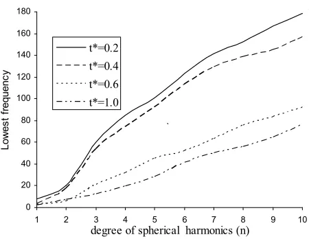
t h R h a b R from Figure 1 that the lowest fre

increase in degree of harmonics. It can be inferred from gree of harmonics the

w

of easing.

hat pation 2

a b

  . It is concluded quency increases with

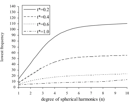
Figure 2 that with increase in de

dissipation of vibration modes go on increasing. Figure 3

the lowest frequency of toroidal vibrations has been plot- ted versus degree of harmonics (n) for different values of thickness to mean radial ratio



* _{, 1}



t . From

Figure 3 it is revealed that e in the degree of harmonics the frequency

0.2, 0.4, 0.6



ith increas

vibrations go on incr milar to t the dissi low (of the o The trends of the profiles in Figure 3 are si as reported in Ding and Chen [17]. But

factor of toroidal vibrations is very rder 10–10₎ F

0 20 120

w

40 60 80

Lo

es

t f

r 100

equenc

140 160 180

y

1 2 3 4 5 6 7 8 9 10

degree of spherical harmonics (n) t*=0.2

t*=0.4 t*=0.6 t*=1.0

`

[image:8.595.311.536.301.475.2]

 

Ω

Figure 1. Lowest frequency of spheroidal vibrations versus degree of harmonics

 

n in (VTE) hollow sphere.

F

0 1 2 3 4 5 6

1 2 3 4 5 6 7 8 9 10

degree of spherical harmonics (n)

di

ss

ipa

ti

on f

ac

tor

7 8 9

t*=0.2 t*=0.4 t*=0.6 t*=1.0

ure 2. Dissipation

Fig

 

D of spher ns versus

degree of harmonics

0 10 20 30 40 50 60 70 80 90 100 110 120 130 140

1 2 3 4 5 6 7 8 9 10

degree of spherical harmonics (n)

lo

w

es

t f

re

que

nc

y

[image:9.595.60.286.78.259.2]

t*=0.2 t*=0.4 t*=0.6 t*=1.0

Figure 3. Lowest frequency of Toroidal vibrations ver- sus degree of harmonics

 

_Ωˆ

 

n in (VTE) hollow sphere in

and behavior of sphere ations and their magnitudes in c

the instant case which is negligible. From the trends of variations of lowest frequency and dissipation factor of S-mode, it is noticed that the thermal variations, thermal relaxation time and viscous nature of the material signi- ficantly affect the characteristics -

cal vibr ontrast to that of

toroidal modes which are only affected due to viscosity but not by the temperature variations as expected.

In Figures 4 to 7, the variations of temperature change (T) and stresses



 rr, r,r



versus









*

r b h

  

i.e. 0





rb h





1 (difference in radius and inner radius to thickness) for the modes



0, 0 , 1,

  

and

 

1, 1 have been plotted in c d ther-mally insulated surface of the (VTE) sphere. Figure 4

revealed that the magnitude of temperature change is though meager, but decreases with increasing values of

 

*

0 ress free an ase of st

 from its maximum value at _* _{0 to become}

steady and stable at the _* _{1in case of all the modes. It}

is inferred from Figure 5 that the variations of radial stress

 

_rr for modes



m n,

    

:

e out with incr

1, 0

ease in val

, 1, 1 initially ues of

in- creases and di

 

_* _{. But} for the mode



0, 0



, the stress is of com

vanishes with i

pressive creasing valu

nature es of and

 

_* its magnitude _{. It is noticed from Figure 6 that the meridian stress} n

 

r of vibration modes



m n,

    

and it dies out

: 1,

with i

0 , 1, 1 has c ncreasing values

of pressi

 

_* _{. Howe}ve nature of this creasing value

ve s

r the mode



0, 0



quantity and its of

 

*

has maximum die out with in-

varia-

tions vibrations

 . Figure

r mode

 

1, 1 . It h s on decreasing

7

as with

shows that the va maximum value

increasing val ria- and ues tion of

its ma of *

stress gnitude

fo goe  to ulti

Figures 8

ma to

tely die out.

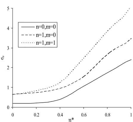
10 represent the variations of displace-ments



ur,u,u



versus

 

*

 for the modes



m n,

 

: 0, 0 , 1, 0

  

and

 

1, 1 . Figure 8 revealed that

the variations of radial disp ement decrease from thei

* lac r

aximum variation with increasing values of

m  0

 

_* tions. place

to become for all modes of vibra-

Figures 9 and the variations of dis- ments

stable at _*

10 sh

1 

ow

u and u versus

 

* . The profiles of

0 0.005 0.01 0.015 0.02 0.025 0.03 0.035 0.04

0 0.2 0.4 0.6 0.8 1

n=0,m=0

T

em

pra

tu

re

C

ha

ng

e

(T

)

n=1,m=0

η*

n=1,m=1

[image:9.595.313.535.134.703.2]

f tem

Figure 4. Variation o perature change

 

T versus

 

_*

of hollow sphere.

Fig.5

-60 -40 -20 0 20 40 60

0 0.2 0.4 0.6 0.8 1

η*

σ

rr

n=0,m=0 n=1,m=0 n=1,m=1

[image:9.595.312.531.161.308.2]

σrr

Figure 5. Variation of stress

 

σrr verses





*

 of hollow sphere.

-250 -200 -150 -100 -50 0 50 100 150 200

0 0.2 0.4 0.6 0.8 1

η*

σr

θ

n=0,m=0 n=1,m=0 n=1,m=1

σrθ

[image:9.595.314.536.353.491.2] [image:9.595.318.525.537.696.2]

Fig.

0 10 30 40 50 60 70

0 0.2 0.4 0.6 0.8 1

η*

r

ϕ

20

σ

n=0,m=0 n=1,m=0 n=1,m=1

[image:10.595.312.535.76.281.2]

σrø

Figure 7. Variation of stress

 

σr verses

 

* of hollow sphere.

0 0.0005 0.001 0.0015

ur

0.002

0 0.2 0.4 0.6 0.8 1

η*

n=0,m=0 n=1,m=0 n=1,m=1

[image:10.595.56.294.76.491.2]

ur

Figure 8. Variation of displacement

 

ur verses

 

*

 of hol- low sphere.

F

0 0.015 0.03 0.045 0.06 0.075

0 0.2 0.4 η* 0.6 0.8 1

u

θ

n=0,m=0 n=1,m=0 n=1,m=1

uθ

Figure 9. Variation of displacement

 

u verses

 

* of hol- low sphere.

0 1 2 3 4 5

0 0.2 0.4 0.6 0.8 1

η*

u

ϕ

n=0,m=0 n=1,m=0 n=1,m=1

[image:10.595.62.283.295.486.2]

σø

Figure 10. Variation between displacement

 

u verses

 

* of hollow sphere.

variations of these quantities show increasing trends with respect to increasing values of _* _{for all the modes of}

vibrations.

5.1. Numerical Data/Information

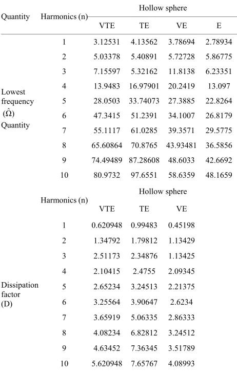
Here in Table 1 shows the Comparison of lowest fre-quency

 



. viscot

al dat

and Dissipation factor (D) in different me-dia i.e hermoelastic (VTE), thermoelastic (TE), vi -

at holl to chec alidity a by using t-test at fixed degree of harmon-ics

s coelastic (VE) and elastic (E) m erials of ow sphere and Table 2 has been given k the v of the numeric



n



us i.e

1, 2, 3

ratio

for different values of thickness to mean radi .



* _{0.2, 0.4, 0.6, 0.8, 1.0}



t  of hollow

5.2. Statistical Analysis

In this sub section we have performed some statistical analysis of computed data for lowest frequency and dis-sipation factor of three harmonics of spher-oidal vibrations in hollow sphere o mean radius ratio

sphere.



n1, 2, 3



of different thickness t

 

t*

t-test has

made from , VE and E materials. The been

order to examine the influence of thermal, viscous and both thermal and viscous, effects on the vibrations.

Y, w eno

y

VTE, TE

used during the analysis in

5.2.1. Lowest Frequency

We take two samples X and here X d tes lowest frequenc

 

ˆ

c (VTE heres

of each mode of vibrations in viscother- oelasti ), thermoelastic (TE) or viscoelastic (VE) hollow sp and Y represents lowest frequency m

 

_ˆ ple in of elastic (E hollow sphere. The size of the sam each case is

) 1

[image:10.595.62.285.521.699.2]