Advanced analytics for the SABR model
∗
A. Antonov and M. Spector
Numerix Quantitative Research
†March 23, 2012
Abstract
In this paper, we present advanced analytical formulas for SABR model option pricing. The first technical result consists of a new exact formula for the zero correlation case. This closed form is a simple 2D integration of elementary functions, particularly attractive for numerical implementation. The second result is an effective approximation of the general correlation case. We use a map to the zero correlation case having a nice behavior on strike edges. The map formulas are easily implemented and do not contain any numerical integration. These formulas are important in volatility surface construction and CMS product replication because they provide correct behavior for far strikes and reduced approximation error. The latter is also helpful for dynamic SABR models.
1
Introduction
The SABR model introduced in Hagan et al. (2002) is widely used by practitioners to capture skew and smile effects of interest rate swaptions. The underlying processFt represents the Constant Elasticity of
Variance (CEV) evolution with log-normal stochastic volatilityvt
dFt=FtβvtdW1
dvt=γ vtdW2
with some correlationE[dW1dW2] =ρdt, powerβ, 0< β <1, and absorbing boundary conditions. The primary usage of the SABR model is volatility surface interpolation. For example, a swaption 1Y10Y with 1Y exercise and 10Y length has several quotes corresponding to different strikes. The SABR model attached to this swaption is calibrated in order to fit existing prices or implied volatilities. The calibrated model is used as an interpolation tool for other strikes.
∗This is version 2 of the paper (July 23, 2011). Here we have updated the numerical experiment tables addressing MC
convergence for small strikes and corrected a typo in the important formula (2.28) (we thank Abdelkader Ratnani for pointing it out). We have also added numerical experiments for the hybrid SABR ZC map. We have explicitly address the approximation procedure at the end of Section 2.2. Other changes are minor.
†Numerix LLC 150 East 42nd Street, 15th Floor, New York, NY 10017; [email protected], [email protected]
Another important application of the SABR model consists of the calculation of European CMS products associated with the swap rate in hand. The CMS price is calculated via integrals of European swaption prices using a static replication formula (Hagan (2003)). The integration is done over swaption strikes from zero to infinity. This means that the SABR swaption pricer should be robust and coherent for all the strikes.
Finally, there is the SABR process application as a term structure model; see, for example, Rebonato et al. (2009) for the SABR/LIBOR Market Model or Mercurio and Morini (2009) for inflation models.
In the original article, Hagan et al. (2002) came up with an approximation formula for European option prices. The logic was based on a small time expansion which was refined later by many other authors, for example, Beresticky et al. (2004), Henry-Labordere (2008), Paulot (2009), Obloj (2008), and others. However, the approximation quality rapidly degrades with time, for example, for maturities larger than 10Y the error in implied volatility can be 1% or more even for ATM values. Moreover, one can easily observe bad approximation behavior for extreme strikes which sometimes prevents obtaining a valid probability density function. These undesired properties on the edges are especially dangerous for CMS calculations by static replication.
The initial Hagan et al. (2002) approximation formula is used as a standard tool for volatility surface interpolation, which has led somehow to the approximation rather than the model itself becoming an industry standard. However, the model price is more coherent and attractive.
A different approach to SABR option pricing was undertaken in Islah (2009) where the author con-tributed an exact formula in terms of a multi-dimensional integration for the zero correlation case and a conditional Bessel process approximation for non-zero correlation. Nevertheless, a practical implementa-tion of Islah’s exact result for calibraimplementa-tion is hardly possible: The final formula consists of three-dimensional integration of special functions and appears to be slow numerically.
Finally, Andreasen and Huge (2011) proposed an approximation-based one-step PDE solver. The procedure was proven to be arbitrage-free (i.e., with valid probability density function), but still delivers an approximation for the SABR model.
In the present article1, we improve the approximate results for SABR option pricing. Namely, our first technical contribution consists of an exact formula for the zero correlation case in terms of a simple 2D integration of elementary functions, or one-dimensional integral of a special function known as McKean kernel. The corresponding integrands have plausible asymptotics which permits an efficient numerical implementation suitable for tight time constraints for calibration.
The second technical result covers a general correlation case where we propose a very accurate approx-imation based on a modelmap procedure. Namely, we calculate effective coefficients of a zero correlation SABR model, the map proxy, such that its small time asymptotics coincide with the initial non-zero correlation case. Note that the efficient coefficient expressions involve simple algebra without numerical integration. Then, we calculate the option price using the effective zero correlation SABR model2; see Antonov-Misirpashaev (2009) for maps to other models.
Our new results provide strongly reduced approximation error and correct behavior on the edges of the distribution for most of model parameters. Note that for very rare situations (large correlations in absolute value and small power parameter) the option price can be occasionally non-convex for small strikes. However, this undesired effect is much less pronounced than that for previous approximations. Moreover,
1The results were first announced in Antonov-Spector (2011).
2Hagan at al. used the Black-Scholes model as the map proxy which has, of course, very different properties than the initial
SABR model.
due to its small amplitude and localization it does not influence CMS pricing by static replication. The high accuracy of our approximation is very important for dynamic SABR models where calibration procedures naturally require a close fit of analytics and real, for example, simulated result. Let us stress that, throughout the paper, we consider the classical SABR model with the stochastic volatilitywithout mean-reversion. This property, however, does not seem to be very intuitive, especially for large time-horizons. Hopefully, our analytical results can be adapted to mean-reverting volatility setups.
The paper is organized as follows. In Section 2, we present the main results. In Section 3, we introduce the SABR Forward-Kolmogorov equation and discuss boundary conditions. Section 4 contains a derivation of the zero-correlation exact results while Sections 5 and 6 are devoted to the general correlation approximation. Finally, we provide numerical results in Section 7 and conclude in Section 8.
2
Main results
Consider the SABR process (Hagan et al. (2002)) for some rate Ft
dFt=FtβvtdW1 (2.1)
dvt=γ vtdW2 (2.2)
with some correlation E[dW1dW2] = ρand powerβ, 0< β <1. The log-normal processvtplays a role
of stochastic volatility. Thus, we have the famous set of five parameters: {F0, v0, β, γ, ρ}. In general, the initial rateF0 is fixed and the parameters{v0, β, γ, ρ}are used for calibration.
A natural choice ofboundary conditions at the zero rate is an absorbing boundary which guarantees the martingale property of the rate. A probability of the rate being at zero is finite: The probability density function (PDF) has a delta-function located at zero.
Below we present advanced analytics for a call option price,
C(T, K) =E[(FT −K)+] (2.3)
or the option time-value
O(T, K) =E[(FT −K)+]−(F0−K)+. (2.4) It is useful to transform the SABR rate processFtto a stochastic volatility Bessel processQtdefined
as
Qt= Ft1−β
1−β. (2.5)
The processQtsatisfies
dQt=
ν+1 2
Q−t1vt2dt+vtdW1 (2.6)
dvt=γ vtdW2 (2.7)
with theBessel index
ν =− 1
2.1
Zero correlation case
In this subsection, we will present results of the zero correlation case. By a change of variables
V = v
γ, V0= v0
γ, t→γ
2t (2.9)
we can setγ= 1 to obtain the normalized form of the SABR evolution
dFt=FtβVtdW1 (2.10)
dVt=VtdW2 (2.11)
with zero correlationE[dW1dW2] = 0.
An option price for zero correlation3can be presented in terms of a simple two-dimensional integral as
C(t, K, F0)−(F0−K)+=
p
KF0e −t/8
√
2πt Z ∞
0
dV V
V
V0
−1/2
1 π
Z π
0
dφsinφ sin(|ν|φ) b−cosφ e
−ξ0(w)2
2t +sin(|ν|π)
π
Z ∞
0
dψ sinhψ b+ coshψe
−|ν|ψe−ξ0(w)2 2t
(2.12)
where we have denoted coefficient
b= q 2
K+q02 2qKq0 depending on the transformed values of the spot and strike
qK =K
1−β
1−β and q0= F01−β
1−β. (2.13)
The function ξ0(w) in the exponent
ξ0(w) = arcosh
q2
K+q20+V2+V02
2V V0 −
qKq0
V V0 coshw
has an argument wdefined differently for the two integrals
coshw= cosφ forφ-integral, coshw= −coshψ forψ-integral.
The integration can be performed numerically in an efficient manner—the integrands are smooth functions of the parameters. Note that the above formula is exact.
We can further simplify the option price formula by introducing the heat kernelG(t, s)
G(t, s) = 2√2e−
t/8
t√2πt
Z ∞
s
du√coshu−coshs u e−u2
2t (2.14)
which is closely related to the McKean (1970) kernelGMK(t, s), namely sinh∂Gs∂s =−2πGMK. The result
is given in the following compact form
C(t, K, F0)−(F0−K)+= 2 π
p
KF0
( Z s+
s−
dssin(|ν|φ(s))
sinhs G(t, s) + sin(|ν|π)
Z ∞
s+
dse−| ν|ψ(s) sinhs G(t, s)
)
(2.15) with the following underlying functions
φ(s) = 2 arctan
s
sinh2s−sinh2s− sinh2s+−sinh2s
(2.16)
ψ(s) = 2 arctanh
s
sinh2s−sinh2s+ sinh2s−sinh2s−
(2.17)
and the integration limits
s−= arcsinh
|qK−q0|
V0
(2.18)
s+= arcsinh
q K+q0
V0
. (2.19)
Note that the option price depends4 on the parametersq
0, qK andV0 through dimensionlesss− ands+. Derivation details can be found in Section 4.
2.2
Non-zero correlation general case
In this subsection, we will announce results for an option price approximation for a general correlation. We will use mathematical results from the heat-kernel theory and will explain it in details later.
For a general correlation, we will use a small-time expansion giving the following formula for the option time-value
O(T, K) = T
3 2
2√2π exp
−12s
2 min
T γ2 −ln
s2 min
2γ2 + ln K
β√v
0vmin− Amin
. (2.20)
Here optimal geodesic distancesminis a function of the initial value of the rate,F0, the initial stochastic volatility valuev0, and the strikeK, defined as follows
smin=
lnvmin+ρv0+γδq (1 +ρ)v0
(2.21)
for
δq= K
1−β−F1−β
0
1−β (2.22)
and
vmin2 =γ2δq2+ 2ργδq v0+v20. (2.23)
The function Aminis the so-called optimal parallel transport
Amin= 1
2ln(K/F0)
β+
Bmin (2.24)
where contribution Bminhas a simple form
Bmin=−12
β 1−β
ρ
p
1−ρ2(π−ϕ0−arccosρ−I) (2.25) with coefficients
L= vmin
q γp1−ρ2 and ϕ0= arccos
−δq γv+v0ρ
min
and integral
I=
2
√
1−L2
arctan√u0+L
1−L2 −arctan
L √
1−L2
forL <1
1
√ L2−1ln
u0(L+√L2−1)+1
u0(L−√L2−1)+1 forL >1
(2.26)
where
q=K 1−β
1−β and
u0=
δq γρ+v0−vmin
δq γp1−ρ2 . See also Henry-Labordere (2008) and Paulot (2009).
The small time expansion works fine for small times, but for moderate and large ones ones it needs to be imroved. We can use the mapping technique (see Antonov-Misirpashaev (2009)) which works as follows. We come up with another model having the same small time expansion for the option (mimicking model) and calculate the final result using the mimicking model. For example, Hagan used the Black-Scholes model or normal one for this. Paulot has proposed the CEV model as the mimicking model. We will go further and use the SABR model with zero correlation (SABR ZC) having similar characteristics and asymptotics to the initial SABR model.
Denote the SABR ZC parameters with tilde and set its skew and vol-of-vol in a strike-independent manner
˜
β = β (2.27)
˜
γ2 = γ2−32nγ2ρ2+v0γρ(1−β)F0β−1
o
(2.28)
and define as usual
δq˜= K
1−β˜−F1−β˜
0
1−β˜ . (2.29)
The initial stochastic volatility value ˜v0 can be calculated as expansion
˜
v0= ˜v(0)0 +Tv˜ (1)
The leading term can be expressed as
˜ v0(0)=
2 Φδq˜˜γ
Φ2−1 (2.31)
where
Φ =
v
min+ρv0+γ δq (1 +ρ)v0
γγ˜
.
The (first) correction to the initial stochastic volatility of the mimicking model can be expressed in an algebraic form of the initial model parameters, the strike, and the leading order value ˜v(0)0
˜ v0(1) ˜ v0(0)
= ˜γ2
1
2(β−β˜) ln(K F0) + 1
2ln (v0vmin)− 1 2ln
˜ v(0)0
q
δq˜2˜γ2+ ˜v(0) 0
2 − Bmin Φ2−1
Φ2+1ln Φ
. (2.32)
Thus, given option strikeK, the coefficients of the initial SABR model, and the postulated free SABR ZC parameters (2.27-2.28), we calculate the effective initial value value of the stochastic volatility as the first order expansion (2.30) with the leading term (2.31) and its correction (2.32). This defines all parameters of the mimicking SABR ZC model. A call option price for the strikeK is thus approximated by the constructed mimicking model—a zero correlation SABR model—for which the analytical option price is available and given by (2.12).
The ATM case is a cumbersome but straightforward limit K →F0. The leading order ATM value reads5
˜ v(0)0
K=F
0
=v0. (2.33)
The first ATM correction can be also expressed in simple terms
˜ v(1)0 ˜ v(0)0
K=F0
= 1 12
1−γ˜
2
γ2 − 3 2ρ
2
γ2+1
4β ρ v0γ F
β−1
0 . (2.34)
Note that its last term comes from the second derivative of the integral B. It can be also found in the formula of Hagan et al. (2002).
We can construct a “hybrid” solution for effective volatilities. Namely, for a general, not necessarily ATM strike, use the optimal strike-dependent leading order initial volatility (2.31) and theATM correction (2.34). We address property of this simple solution in the Section 7.
The general caseβ6= ˜β is slightly more complicated resulting in the following leading order effective volatility
˜ v0(0)
K=F0
=v0Fβ− ˜
β
0 (2.35)
and its correction
˜ v(1)0 ˜ v(0)0
K=F0
= 1 12
1−γ˜
2
γ2 − 3 2ρ
2γ2+1
4β ρ v0γ F
β−1 0 +
1 24v
2 0F
2β−2 0
(β−1)2−( ˜β−1)2. (2.36)
Finally, we summarize the approximation procedure. Given the SABR model with non-zero correlation (2.1-2.2), strikeK and maturityT, we come up with (strike dependent) mimicking process ˜Ftand ˜vt
dF˜t= ˜F
˜
β
t ˜vtdW˜1 (2.37)
dv˜t= ˜γ˜vtdW˜2 (2.38)
with zero correlation between the driving Brownian motions E[dW˜1dW˜2] = 0. The efficient parameters are calculated as follows: the skew ˜β = β, the vol-of-vol ˜γ as (2.28) and the initial (strike dependent) effective volatility ˜v0= ˜v0(0)+Tv˜
(1)
0 as (2.31-2.32). The approximate call option price
C(T, K)≃E[( ˜FT −K)+]
is finally computed by the numerical integration (2.15) or other equivalent formula.
2.3
Asymptotics
In this section, we consider the vol-of-volγ as not being unity and operate with processvt(2.7) instead
ofVt(2.11) and corresponding stretched timetγ2.
Being equipped with an exact solution for the zero correlation case, we can obtain asymptotics for small and large strikes. Below we present the results in terms of the Bessel form of the SABR process (2.6) where we have replaced the SABR processFt byQt= F
1−β t
1−β. Obviously, the initial SABR density
function P(t, F) =E[δ(Ft−F)] can be related with the Bessel process PDFP(t, q) =E[δ(Qt−q)] by dF P(t, F) =dqP(t, q).
At the end of section 4.1, we have derived small strike behavior, which we present here forγ6= 1
p(t, q|q0) = 4q
(|ν|+ 1)v2
0(γ q0)2|ν|+2e−tγ 2/8
−2πip
2πtγ2
Z ∞
0
dv v0
v0
v
1/2Z ∞ −∞
dξsinhξ e−(ξ2+tγiπ2)2
(γ2q2
0+v2+v20+ 2vv0coshξ)|ν|+2
.
The asymptotic is linear inq. However, we did not manage to simplify the coefficient which is, of course, positive and real in spite of a presence of the imaginary unit.
Section 4.3 gives a leading order of large strike asymptotics
p(t, q)∼e−2tγ12 ln2 2 q γ
v0 (2.39)
which coincides with that given by the heat-kernel small time expansion (2.20) where the geodesic distance smin∼ln(2vq γ0 ). One can also “quantify” the notion of thelarge qand the strike
q∼vγ0e3γ√t (2.40)
or, in terms of the strikes
K∼ (1
−β)v0
γ
1−1β
e3γ
√ t
1−β. (2.41)
See Section 4.3 for details. A log-volatility of a rate is of order of 20%, thusv0∼0.2F01−β. The vol-of-vol can have also the same order of 20%−40%. Thus, a large strike is approximately
K∼F0 (1−β) 1 1−β e
√ t
Accordingly, for smallβ (corresponding to the “normal” case) the distribution is quite narrow even for moderate maturities. On the other hand, a log-normal case β → 1 gives very fat wings and a “large strike” can exceed the initial rate value by multiple orders.
For the general correlation case, one can show that the PDF will retain linear asymptotics in q for small strikes
p(t, q)∼q. (2.43)
See Section 3. For large strikes, the leading asymptotics correspond to its small-time counterpart obtained by the heat-kernel small time-expansion
p(t, q)∼e−2tγ12 ln 2 2q γ
(1+ρ)v0. (2.44)
This is an intuitive result without a strict proof, however.
The approximation gives a close fit for the distribution for a wide range of strikes. However, very rarely, the approximate PDF can have small negative values for small strikes (for smallβ and largeρ). Of course, these negative values are tiny w.r.t. huge negative probabilities for existing approximationa based on the effective implied volatility. For large strikes, our approximation numerically appears to be close to the heat-kernel small time expansion (2.44); we will address it rigorously elsewhere.
3
SABR density PDE: absorbing and reflecting solutions
In this section, we study the SABR density general properties. Starting with the SDE for the Bessel process with stochastic volatility (BES SV) (2.6), we address boundary conditions in terms of the PDF behavior at zero, identify them with absorbtion and reflection, and comment on the norm and moment conservation.
The BES SV process gives rise to the Forward Kolmogorov equation
pt=−
ν+1 2
v2 q−1p q+
1 2v
2p
qq+ργ v2pqv+
1 2γ
2 v2p
vv (3.1)
which delivers a solution for the density p(t, q, v) = E[δ(qt−q)δ(vt−v)] with the initial condition p(0, q, v) = δ(q0−q)δ(v0−v). The solution is unique provided that certain boundary conditions are imposed atq= 0.
As in the pure Bessel case, see, for example, Jeanblanc et al. (2009), we look for a solution at smallq in the form
p(t, q, v) =qκφ(t, q, v)
where function φ(t, q, f) is regular atq= 0. A balance of leading terms (of the order ofqκ−2) determines two possible characteristic exponents,κ1= 1 andκ2= 2ν+1, and thus gives rise to the following solutions
p(1)=q C0+C1q+O(q2), (3.2)
p(2)=q2ν+1 B0+B1q+O(q2). (3.3) Note that the second one may be realized only for ν > −1 as follows from the integrability condition, 2ν+ 1>−1. Considering the next order leads to
v2C1=− 2ρ 1−2ν v
2C 0v
For the zero correlation the first order coefficients cancel out.
Let us examine these asymptotics of being absorbing or reflecting. We notice that the marginal distribution of the stochastic volatilityvtis log-normal
p(t, v) =
Z
dq p(t, q, v) = p 1
2πtγ2 v
−1e−1 2
(lnv+ 12tγ2)2
tγ2 . (3.5)
This means that for any fixed q the PDF p(t, q, v) goes to zero forv→0 with all its derivatives overv. This property permits us to understand the asymptotic behavior of the marginal distribution ofqt
p(t, q) =
Z
dv p(t, q, v). (3.6)
Indeed, integrating the Forward Kolmogorov equation over v, we obtain6
∂tp(t, q) = Z
dv v2
−
ν+1 2
q−1p q+
1 2pqq
. (3.7)
A time dependence of the norm
n(t) =
Z
dq dv p(t, q, v)
is established by the integration of the equation (3.7) over q and occurs to be dependent on the PDF behavior at the q= 0 boundary,
∂tn(t) = Z
dv v2
ν+1 2
q−1p−12pq
q→0
. (3.8)
For the solution (3.2), we get
∂tn(1)(t) =ν Z
dv v2C 0(t, v) while for the solution (3.3) the factor to be integrated becomes
ν+1 2
q−1p−12pq
q→0
=−12q2ν+1(B1+O(q))
and does not necessarily turn into zero at q → 0. Indeed, we have −1 < 2ν+ 1 < 0 in the interval 0< β < 1
2. However, integrating over vcancels the potentially singular term due to (3.4)
Z
dv v2B1(t, v) =−2ρ
Z
dv v2B0v = 0
and results in the norm conservation
∂tn(2)(t) = 0.
Thus, the norm-conserving solution p(2) (3.3) is naturally identified as reflecting, and the solution p(1) (3.2) which reveals the norm defect (at negativeν) is identified as absorbing.
6We used the boundary properties of the density forv
Though interested mainly in negative indexν (β <1), we comment briefly on the caseν >0. Imagine that the total PDF is presented by some combination of the solutions p(1) and p(2). For small q, the leading term of p(1)∼qdominates the leading term ofp(2) ∼q2ν+1 implying that
p=p(1)+p(2)≃C 0(t, v)q
∂tn(t) =∂tn(1)(t) +∂tn(2)(t) =ν Z
dv v2C0(t, v).
These relations, however, are in conflict. On the one hand,C0must be positive to define positive PDFp. Both ν andC0 being positive, the time derivative of the norm must also be positive, ∂tn(t)>0, which
is probabilistically impossible. Indeed, if the initial distribution is normalized to one,n(0) = 1, the norm n(t) has no room to grow farther. Thus, the absorbing solutionp(1)may be realized only atν <0 (β <1). In this case, the norm defect,∂tn(t)<0, merely indicates that there is a finite probability for processqt
to be at zero which is natural for the absorbing solution,P(qt= 0) = 1−n(t).
We conclude that for a positive indexν >0 (β >1) there exists only reflecting solutionp(2) while for
ν <−1 (1
2 < β <1) the only possible solution is the absorbing onep
(1). In these intervals of the index
ν the PDFpis completely determined by the inner dynamics of the random processesqtand vtwith no
freedom for an outside boundary condition at q= 0. In the interval−1< ν <0 (β < 12) both solutions are legitimate, and we have to impose a boundary condition atq= 0 to select the proper unique solution. As we have seen, a selection of the reflecting solution is associated with the requirement of the norm conservation. Below we prove that a selection of the absorbing solution (and ignoring the reflecting one) is related with the martingale property of the SABR processFt. Indeed, in terms of the BES SV process
we need to calculate the (−2ν)-th momentm−2ν(t) as far as the rate process reads Ft=q−t2ν(−2ν)2ν.
Multiplying the Forward Kolmogorov equation (3.1) byq−2ν and rearranging terms we obtain
q−2νpt=
1 2v
2 q−2ν+1(p q−1)
qq+
ργ q−2ν v2p q+
1 2γ
2q−2ν v2p v
v
. (3.9)
Thus, the moment time-derivative
∂tm−2ν(t) = Z
dq dv q−2νp
t(t, q, v) =−
1 2
Z
dv v2 q−2ν+1(p q−1)
qq=0 (3.10)
has the following form for each of the solutionsp(1) andp(2) ∂tm(1)−2ν(t) = 0
∂tm(2)−2ν(t) =−ν Z
dv v2B0(t, v).
This indicates that the SABR process is a global martingale for the absorbing solution and a strict local one for the reflecting solution.
Below we will consider the SABR model withabsorbing boundary as the most coherent and standard one.
4
Zero-correlation formulas
Before starting our analysis, transform (2.5) the rate process Ft into the Bessel process Qt, which
satisfies
dQt =
ν+1 2
Q−t1Vt2dt+VtdW1 (4.1)
dVt = VtdW2. (4.2)
The zero correlation permits “absorbing” the stochastic volatilityVtinto the new stochastic timeτ
τt= Z t
0
V2
t′dt′. (4.3)
Indeed, the new process
dB1τ =VtdW1t
is a Brownian motion in timeτ
h(dB1τ)2i=Vt2h(dW1t)2i=Vt2dt=dτ.
Process B1τ also remains uncorrelated with W2. Denote the process Qt measured in the new time τ by Rτ≡Qt. Its governing SDE looks like
dR= (ν+1 2)
dτ
R +dB1τ. In other words, the processRτ is a Bessel process with indexν.
4.1
The marginal PDF
In this subsection, we address the marginal distribution of the BES SV processQtdefined as
p(t, q |q0, V0) =E{W2}E{W1}{δ(Qt−q)|q0, V0} =E{W2t}
E{B1τ}{δ(Rτ−q)|q0}
|V0 . (4.4)
We concentrate on the PDF for q > 0 because the call option price does not depend on the (finite) probability ofQt= 0.7
SinceB1τ remains uncorrelated withW2t, the inner average is the single point PDF of Bessel process BES(ν) with negative index ν and absorbing boundary condition (see, for example, Jeanblanc et al. (2009))
p(ν)(τ, q|q0) = 2q
e−q2 +q
2 0 2τ 2τ
q
q0
ν
I−ν qq0
τ
(4.5)
forq >0.
The marginal PDF can be expressed in terms of the stochastic timeτt densityp(t, τ) =E[δ(τt−τ)]
p(t, q|q0, V0) =E{W2t}
n
p(BESν) (τt, q|q0)
o
=
Z ∞
0
dτ p(BESν) (τ, q|q0)p(t, τ). (4.6)
7The finite probability
P[Qt = 0] for our absorbing boundary condition can be computed requiring the unit norm, i.e.
One can calculate the density p(t, τ) from the joint distribution function of τt and Vt, p(t, τ, V |V0) =
E[δ(τt−τ)δ(Vt−V)], obtained by Yor (1992). Thus, to calculate the marginal PDFp(t, q|q0) we can proceed as follows
p(t, q|q0) =
Z
dτ p(ν)(τ, q|q0)
Z
dV p(t, τ, V |V0).
We recall here the Yor result8
p(t, V2, τ |V02) =
e−t/8
V2
V2
V2 0
−1/4 e−V2 +V
2 0 2τ 2τ ϑ
V V
0
τ , t
(4.7)
where functionϑ(r, t) is defined as
ϑ(r, t) = re π2
2t
π√2πt
Z +∞
0
e−rcoshξ−ξ22t sinhξsinπξ
t dξ (4.8)
= r
(−2πi)√2πt
Z +∞ −∞
e−rcoshξ−(ξ+2iπt)2 sinhξ dξ. (4.9) Despite looking different, two last expressions are equal, as readily seen by developing the exponent exp−(ξ+2iπt)2
and keeping only the even part of the integrand in (4.9). The more compact form (4.9) may be preferable when making various transforms and trying to use analytical properties of functions after moving into complex plane ξ.
In Appendix A, we describe a simple derivation of the joint PDF ofV2
t and τt based on arguments
close to Yor’s. The key elements include the Laplace transform (LT) in time which represents, in essence, passing to a random exponential time. Then, we make use of the Lamperti property of a geometric Brownian motion, which states that a geometrical Brownian motion
Xt(ν)= exp(2νt+ 2Wt)
measured in the stochastic timeτt=R0tXt′dt′, becomes a Squared Bessel processX (ν)
t ≡ρ
(ν)
τt with index
ν (not to be confused withν used earlier for processQt). Next, we apply the Girshanov theorem which
allows us by change of measure to eliminate “path-dependent” factors. As a result, the LT of the joint PDF (4.7) proves to be proportional to the distribution of a Bessel processρ(τµ)with indexµ= (ν2+2λ)1/2
depending on the Laplace parameter λand the original indexν. Finally, the inverse Laplace transform leads to the expressions (4.7-4.8).
Thus, we come up with the following expression for the joint PDF ofQtandVt
p(t, q, V |q0, V0) = 2V
e−t/8
V2
V
V0
−1/2Z ∞
0
dτ p(ν)(τ, q|q0)
e−V2+V02 2τ 2τ ϑ
V V
0
τ , t
. (4.10)
Note inter alia that it is possible to present the LT of the joint density ofQtandVtin a compact and
nice convolution form
ˆ
p(λ, q, V |q0, V0) = 1 V2
V
V0
−(µ+1/2) Z ∞
0
dτ p(BESν) (τ, q|q0)p(BESµ) (τ, V|V0) (4.11)
8We have denoted the PDF of the stochastic timeτ and the
squareVt2 asp(t, V2, τ |V02) =E
for µ = (14 + 2λ)1/2. To our knowledge, this formula is new but we will not use it in our option price derivation.
Integrating the joint density (4.10) over volatilityV, we obtain a marginal distribution ofQt
p(t, q |q0) =e−t/8
Z ∞ 0 2dV V V V0
−1/2 Z ∞
0
dτ p(ν)(τ, q|q0) e
−V2+V
2 0 2τ 2τ ϑ
V V
0
τ , t
. (4.12)
At the end of this subsection, we address the smallq (or smallF) expansion. Indeed, we obtain the leading term ofp(ν)(τ, q|q
0) forq→0, the PDF of the Bessel process (4.5), taking into account the small argument asymptotics of the Bessel functionI−ν(x)
p(ν)(τ, q|q0)≃ 1 Γ(|ν|+ 1)
q τ
q2 0 2τ
|ν|
e−q
2 0 2τ. Then, substitute it into the formula (4.12)
p(t, q|q0)≃ 2q Γ(|ν|+ 1)e
−t/8Z ∞ 0
2dV V
V
V0
−1/2 Z ∞
0
dτ (2τ)2
q2 0 2τ
|ν|
e−
q20 +V2+V02 2τ ϑ
V V
0
τ , t
.
Next, using expression (4.9) for the functionϑ, we can integrate overτ
Z ∞ 0 dτ τ 1 2τ
|ν|+2
e−A
2τ = Γ(|ν|+ 2)
A|ν|+2 resulting in a linear asymptotic in q
p(t, q|q0)≃4q(|ν|+ 1)V 2 0 q2 0 Z ∞ 0 dV V0 V V0
−1/2
Z ∞
−∞
dξ sinhξ
−2πi
q2
0
q2
0+V2+V02+ 2V V0coshξ
|ν|+2 e−(ξ+2iπt)2−t/8
√
2πt ,
confirming our general result derived for any correlation. Unfortunately, the integral coefficient can hardly be simplified.
4.2
Option pricing
Integrating the marginalqdistribution with a given payoff generates the option price in the form
Csabr(t, K, F0) =e−t/8
Z ∞ 0 2dV V V V0
−1/2Z ∞
0
dτ Ccev(τ, K, F0)e
−V2+V
2 0 2τ 2τ ϑ
V V0
τ , t
(4.13)
where Ccev(τ, K, F0) is the τ-time value of the corresponding option in the CEV model.
probability density. (Note that, in the case of β < 1/2 with reflection, his formulas are incorrect.) Altogether, it included four integrations, of which one, over stretched time (ourτ), was taken analytically. Final results of Islah contain triple integrals to be computed numerically: integration with respect to F which originates from integrating χ2 probability density, integration with respect to volatility V and integration with respect to parameterξ according to the definition of the Yor functionϑ.
Drawbacks of this approach include complicated integrands, too many (three) numerical integrations, and general convergence problems with integration overξat small timest. Regarding the latter, we notice that explicitly real integral form for functionϑ(r, t) (4.8) contains two problematic factors, especially, for small maturities. One factor is sinπξt which may oscillate very fast and another one,eπ22t, may take huge values. This requires an extreme accuracy in numerical computation as discussed by Carr and Schroder [6] in the context of Asian options.
We have found ways to significantly simplify expressions for option values, coming up with a double integral of elementary functions. (It may even be considered as a single integral if we accept the heat kernel function involved,G(t, s), as given – see below.) The basic idea is to transform expression (4.12) for the marginal distribution of q before integrating it with the payoff. Namely, we integrate (4.12) by parts with respect toτ, in order to get τ-time derivative∂τp(τ, q), then express∂τpthrough the proper
evolution operator using the forward Kolmogorov equation. After that, integration with payoff over F becomes trivial. Subsequent integration over stretched timeτleaves only a double integral to be computed numerically. Another essential attainment is related to integration with respect toξby making use of the complex (rather than real) integral form of the Yor function ϑ(4.8). Continuing the function involved into the complex plane ξ, we have managed to shift the path of integration overξ downward from the real axis onto the horizontal line ξ =u−iπ with realu, thus converting the ‘trouble making’ function exp{−(ξ+2iπt)2}into the pure real and decaying exponent exp{−
u2 2t}.
Leaving the derivation details to Appendix B, we present some equivalent expressions for the call option value
C(t, K, F0)−(F0−K)+=
p
KF0e −t/8
√
2πt Z ∞
0
dV V
V
V0
−1/2
1 π
Z π
0
dφsinφ sin(|ν|φ) b−cosφ e
−ξ0(w,V)2
2t +sin(|ν|π)
π
Z ∞
0
dψ sinhψ b+ coshψe
−|ν|ψe−ξ0(w,V)2 2t
(4.14)
with coefficientb=q2K+q02
2qKq0 and function
ξ0(w, V) = arccosh
q2
K+q20+V2+V02
2V V0 −
qKq0
V V0 coshw
(4.15)
defined in the following way for two integrals
coshw= coshiφ= cosφ forφ-integral, coshw= cosh(±iπ+ψ) =−coshψ forψ-integral.
An integration overV gives rise to a heat-kernel looking function
G(t, s) = 2√2e
−t/8
√
2πt
Z ∞
s
d(√coshu−coshs)e−u
2 2t = e
−t/8
√
πt
Z ∞
s
du√ sinhu
coshu−coshse −u2
2t. (4.16) Note that its derivative, −1
2π ∂G(t,s)
sinhs∂s =GMK(t, s), coincides with the McKean heat kernelGMK(t, s) on
the Poincare hyperbolic plane H2. Note also that the following alternative form of the function G(t, s) obtained from (4.16) by integration by parts
G(t, s) = 2√2e−
t/8
t√2πt
Z ∞
s
du√coshu−coshs u e−u
2
2t (4.17)
is convenient for numerical computations. Thus, the option price looks like
C(t, K, F0)−(F0−K)+= 1
π
p
KF0
Z π
0
dφsinφ sin(|ν|φ) b−cosφ
G(t, s(w)
D(w) (4.18)
+ sin(|ν|π)
Z ∞
0
dψ sinhψ b+ coshψe
−|ν|ψG(t, s(w) D(w)
.
Other parameters and functions involved are defined as follows:
D2(w) =2qKq0 V2
0
(b−coshw) + 1
s(w) =arccoshD(w). (4.19)
Finally, we can simplify the option price formula using a new integration variables
C(t, K, F0)−(F0−K)+= 2 π
p
KF0
( Z s+
s−
dssin(|ν|φ(s))
sinhs G(t, s) + sin(|ν|π)
Z ∞
s+
dse−| ν|ψ(s) sinhs G(t, s)
)
(4.20) with the following underlying functions
φ(s) = 2 arctan
s
sinh2s−sinh2s− sinh2s+−sinh2s
(4.21)
ψ(s) = 2 arctanh
s
sinh2s−sinh2s+ sinh2s−sinh2s−
(4.22)
the integration limits
s−= arcsinh
|qK−q0|
V0
(4.23)
s+= arcsinh
q K+q0
V0
(4.24)
4.3
Asymptotics at large strikes
Full calculation of asymptotics for large strikes turned out to be complicated and will be addressed elsewhere; here we give its leading term.
The dominating term in the option price integrand (4.20) is the kernelG(t, s) with strongly decreasing Gaussian asymptotics. Indeed, make in (4.16) a substitution
u=ps2+w2≃s
1 + w 2 2s2
=s+w 2 2s.
Then
coshu≃coshs+w 2 2s sinhs
√
coshu−coshs≃ r
sinhs
2s w 1 +O(s −1)
and the asymptotic ofG(t, s) looks like
G(t, s) = 2√2
r
sinhs 2s
e−t/8
√
2πt
Z ∞
0
dw e−s2+w
2
2t 1 +O(s−1)=
r
sinhs s e
−s2 2t−
t
8 1 +O(s−1). (4.25)
The leading asymptotics of the option price comes from the termG(t, s) corresponding to larges∼s−∼ s+ which, for simplicity, we define as
s0= ln 2qK
V0
. (4.26)
We see that the resulting leading asymptotics
C(t, K, F0)∼G(t, s0)∼e− s20
2t for K→ ∞ (4.27)
coincide with that given by the Heat-Kernel small time expansion (2.20) where, for large strikes,smin∼s0. We doubt, however, that the pre-exponential factors of these two different limits,K→ ∞andt→0, will also coincide.
Given the Gaussian nature of the decay we can quantify larges0as being
s0∼3
√
t (4.28)
or, in terms of the qK,
qK ∼V0e3
√
t (4.29)
or, in terms of the strikes,
K∼((1−β)V0) 1 1−β e3
√ t
5
Heat-kernel expansion for SABR density
The heat-kernel expansion (DeWitt (1965)) is a small-time approximation for the probability density function (PDF). This is a regular recipe for general stochastic systems (see the review of Avramidi [4]). The PDF expansion for the SABR model was calculated in Henry-Labordere (2008) and Paulot (2009). It can be written in our (q, V) variables (2.5) as9
p(q, v) = 1 γv2p
1−ρ2 1 2πt
s
s(q, v)
sinhs(q, v)P(q, v)e
−s2(2γq,v2t)(1 +O(t)) (5.1)
where geodesic distance s(q, v) from the leading term depends on the volatility of the processes Qt and vt, and parallel transportP(q, v) depends on the drifts.
Before proceeding with details, we notice that the distance and the parallel transport do not depend on time. It is also worth mentioning that the heat kernel does not take into account the boundary conditions: for small time, the rate “cannot” approach the boundary.
In principal, it is possible to obtain the higher orders in time10, however, the formulas are very complicated (see Paulot (2009)).
To define the distance and the parallel transport, we introduce new variables (on the so-called hyper-bolic plane)
x=q−
v γcosα
sinα (5.2)
y= v
γ (5.3)
with
ρ= cosα. (5.4)
The distancesis defined in terms of the variables (x, y) as
coshs= (x−x0)
2+ (y−y 0)2
2yy0 + 1
or in terms of (q, v)
coshs=[γδq−ρ(v−v0)] 2 2(1−ρ2)v v
0
+(v−v0) 2 2vv0
+ 1. (5.5)
Proceed now to the parallel transport, also defined by its logarithmA
P =e−A.
Loosely speaking, the term Ais an integral of the system drift over the most probable path connecting initial point (q0, v0) and final point (q, v). Detailed consideration permits one to express the parallel transport as
A=−(ν+ 1/2) ln
q
q0
+B= 1 2ln
F
F0
β
+B (5.6)
where Bis the following integral
B=−12
β 1−β
ρ (1−ρ2)
Z
C
−ρdq′+dV′
q′ (5.7)
along the geodesic line C from original to current point, i.e., the most probable path. It occurs that the geodesic line is a semi-circle in coordinates (x, y) with center (xc,0)
xc= x+x0
2 +
y2−y2 0 2(x−x0)
(5.8)
and radiusR
R2=
(x−x0)2+y2+y02
2
−4y2y2 0 4(x−x0)2
. (5.9)
The curveC is parameterized via the angle on the circle, i.e. a point (x′, y′) lying on the geodesic line is expressed via the angleϕ′
x′=x
c+Rcosϕ′ y′=Rsinϕ′.
The angles corresponding to the initial (x0, y0) and final points (x, y) are
ϕ= arccosx−xc R
ϕ0= arccosx0−xc
R
and satisfy
0≤ϕ0≤ϕ′ ≤ϕ≤π. (5.10)
The integral B(5.7) can be transformed to
B = 1
2
β
1−βcotα
Z
C
−cosα dx′+ sinα dy′ q0+ (x′−x0) sinα+ (y′−y0) cosα
(5.11)
= −1 2
β 1−β cotα
Z ϕ
ϕ0
Rsin(ϕ′+α)dϕ′
q0−Rsin(ϕ0+α) +Rsin(ϕ′+α)
. (5.12)
Finally, denoting
L−1=q0
R −sin(ϕ0+α) =
xc sinα
R , (5.13)
we conclude that
B=−1 2
β
1−β cotα
ϕ−ϕ0−
Z ϕ+α ϕ0+α
dϕ′
1 +Lsinϕ′
. (5.14)
6
General correlation approximation formulas
In this Section we will apply the mapping technique (see Antonov-Misirpashaev (2009)) which works as follows. To approximate an option price C(T, K) =E[(FT −K)+] we come up with another mimicking model orproxyF˜t, having the same small time expansion for the option. The mimicking model is supposed
to have an exact expression for its option price. The final result is calculated using the mimicking model
C(T, K)≃E[( ˜FT −K)+].
For example, Hagan used the Black-Scholes model or normal one for this. Paulot has proposed the CEV model as the mimicking model. We will go further and use the SABR model with zero correlation (SABR ZC) having similar characteristics and asymptotics to the initial SABR model.
First, we represent the SABR rate PDF using the BES SV PDF (5.1)
P(t;F, v)≃2πtγ1 1
v2Fβp
1−ρ2
r
s sinhsPe
− s2
2tγ2. (6.1)
Then, we apply Ito’s lemma to a process (Ft−K)+ which gives, after averaging,
E[(FT −K)+] = (F0−K)++ 1 2
Z T
0
dtE[δ(Ft−K)Ft2βv2t]. (6.2)
The average under the integral can be rewritten as
E[δ(Ft−K)Ft2βvt2] =K2β Z
dv P(t; K, v)v2 (6.3)
and taken using the saddle point for small times
Z
dv f(v)e−
s2(F0,v0 ;K,v) 2tγ2
≃γp2πt(1−ρ2)v 0vmin
r
sinhsmin
smin e
−s
2 min 2tγ2 f(v
min) (6.4)
where
vmin2 =δq2γ2+ 2ρδq γ v0+v02 (6.5) and
smin=
lnvmin+ρv0+δq γ (1 +ρ)v0
(6.6)
for
δq= 1 1−β
K1−β−F1−β
0
. (6.7)
Thus,
E[δ(Ft−K)Ft2βvt2] =
1
√
2πtK β√v
0vmine− s2min 2tγ2
Pmin (6.8)
where
The integration over time (6.2) can be done analytically. Indeed, for smallT, Z T 0 dte −1 2 s2 tγ2 √
t = 2s γ −1Z ∞
s γ√T
dx x2e
−1 2x
2
≃γ2T
3 2
s2 2
e−12 s 2
T γ2. (6.10)
Thus, the option time-value
O(T, K) = T
3 2
2√2π exp
−12s
2 min
T γ2 −ln
s2 min
2γ2 + ln K
β√v
0vmin− Amin
. (6.11)
The integral termBmin in the parallel transport (5.6)
Amin= 1 2ln
K
F0
β
+Bmin (6.12)
simplifies whenv=vmin. Indeed,
φ+α=π (6.13)
which is equivalent to
q=xcsinα (6.14)
or
y=Rsinα. (6.15)
The parameter Lcan be also simplified:
L= y
qsinα = vmin
q γ sinα. (6.16)
Then the parallel transport integral (5.14) transforms to
Bmin=
Z
Bidxi=−12 β
1−β cotα
π−ϕ0−α−
Z π
ϕ0+α
dϕ′
1 +Lsinϕ′
. (6.17)
The underlying integral can be easily taken analytically. Indeed, after variable changeu= cotϕ2′, we have
I≡ Z π
ϕ0+α
dϕ′
1 +Lsinϕ′ = Z u0
0
du
1 +u2+ 2L u (6.18)
where we used relations sinϕ′= 2u/(1 +u2) anddϕ′=−2du/(1 +u2) and denoted
u0= cotϕ02+α. The latter integral reads
I= 2 √
1−L2
arctan√u0+L
1−L2 −arctan
L √
1−L2
forL <1,
1
√ L2−1ln
u0(L+√L2−1)+1
u0(L−√L2−1)+1 forL >1.
Note that we can express the underlying parameteru0in simple terms
u0= cotϕ02+α =
δq γρ+v0−vmin
δq γp1−ρ2 using
sin(ϕ0+α) =−δq
R and cos(ϕ0+α) =−
δqcosα+v0
Rsinα . (6.20)
6.1
Map to the CEV model
We describe here how to do the map to the CEV model (see also Paulot (2009)). First, calculate the time-value expansion of the CEV mimicking model,
dF˜ = ˜Fβ′
σdW ,˜ (6.21)
with possibly different powerβ′ with respect to the SABR power. The CEV PDF expansion reads (see,
for example, Jeanblanc et al. (2009))
pCEV(t, F)≡E[( ˜Ft−F)] =√ 1
2π t σ2F
−β′
e−
F1−β′ −F1−β′
0
2 2t σ2 (1−β′)2
F F0 −β ′ 2 . (6.22)
The integrand underlying the option price
E[( ˜FT −K)+] = (F0−K)++1 2
Z T
0
dtE[δ( ˜Ft−K) ˜F2β
′
t σ2] (6.23)
is simply
E[δ( ˜Ft−K)F2β
′
t σ2]≃ σ2
√
2π t σ2e
−
K1−β′ −F01−β′
2
2t σ2 (1−β′)2 (K F 0)
β′
2 (6.24)
where CEV geodesic distance is
sCEV = K1−β′
−F01−β′
1−β′ . (6.25)
The option time-value can be calculated as follows
˜
O(T, K) ≡ 12 Z T
0
dtE[δ( ˜Ft−K)F2β
′
t σ2]≃
1 2σ
2 (K F 0)
β′ 2
Z T
0
dt√ 1
2π t σ2e
−s
2 CEV
2t σ2 (6.26)
= 1
2σ 2 (K F
0) β′
2
Z T
0
dt√ 1
2π t σ2e
−s2CEV
2t σ2 (6.27)
≃ T
3 2
2√2π exp
−12s
2
CEV
T σ2 + lnσ−ln
s2
CEV
2σ2 +
β′
2 ln (K F0)
. (6.28)
To make a fit with SABR, we should equate
1 2
s2CEV
T σ2 −lnσ+ ln
s2CEV
2σ2 −
β′
2 ln (K F0) = 1 2
s2min
T γ2 + ln
s2min
2γ2 −ln K
β√v
Consider now expansion of the CEV volatility
σ=σ0+T σ1+· · ·
We obtain the following condition, zeroing T−1coefficients
s2
CEV T σ2 =
s2 min
T γ2 ⇒ σ=γ
sCEV smin
. (6.30)
Expanding σin s2CEV
T σ2 , we get a condition for free terms equal to zero
−s
2
CEV σ2
0
σ1
σ0 − lnσ0−
β′
2 ln (K F0) =−ln K
β√v
0vmin+Amin (6.31)
giving the CEV volatility correction
σ1
σ0 =
ln Kβ√v
0vmin− Amin−lnσ0−β ′
2 ln (K F0)
s2 CEV
σ2 0
. (6.32)
To obtain the effective BS volatility expansion, we should calculate the limitβ′ →1. The BS geodesic
distance reads
sBS= sCEV|β′=1=
ln K F0
giving the leading volatility term
σ0=γ
ln
K F0
smin and the first volatility correction
σ1
σ0 =
ln Kβ√v
0vmin− Amin−lnσ0−12ln (K F0)
s2 min
γ2
.
In the ATM limit the effective BS volatility expansion terms read
σ0|K=F0=v0F
β−1 0 and
σ1
σ0
K=F0
= 1 24v
2
0(1−β)2F 2β−2 0 +
1
4v0ρ γ β F
β−1 0 +
1 12γ
2−1 8ρ
2γ2
6.2
Map to the zero correlation SABR model
Zero correlation SABR process represents a better choice of the mimicking model (proxy). Indeed, it has close properties with a general correlation SABR and possesses an analytical solution for option price. Denote the mimicking model parameters with a tilde (2.37-2.38). To find them, we should match the option price expansion (6.11) between the initial SABR and its zero correlation proxy
1 2 ˜ s2
min
T˜γ2 + ln ˜ s2
min 2˜γ2 −ln
Kβ˜pv˜0v˜min
+ ˜Amin= 1 2
s2 min
T γ2 + ln
s2 min
2γ2 −ln K
β√v
0vmin+Amin. (6.33)
We fix the vol-of-vol ˜γand the power ˜β in the mimicking model and look for time-expansion of the initial volatility
˜
v0= ˜v(0)0 +Tv˜ (1)
0 +· · · (6.34)
Denote the function appearing in the argument of the logarithm of the optimal geodesic distance (6.6) as
φ= vmin+ρv0+γδq (1 +ρ)v0
, (6.35)
i.e., smin=|lnφ|. Similarly, for the zero correlation, ˜smin(˜v0) =|ln ˜φ(˜v0)|, we have
˜ φ(˜v0) =
s
1 +
δq˜˜γ ˜ v0
2
+δq˜˜γ ˜ v0
(6.36)
where
δq˜=K
1−β˜−F1−β˜
0 1−β˜ .
To organize the fit (6.33) in the main order, we should find the leading order of the mimicking-model initial volatility (6.34) such that the equation
1 2 ˜ s2 min ˜ v(0)0
Tγ˜2 = 1 2
s2 min
T γ2 (6.37)
is satisfied. A solution of this equation follows from the fit condition ˜φ˜v0(0)
=φ˜γγ ˜
v0(0)=
2 Φδq˜˜γ
Φ2−1 (6.38)
where we have denoted Φ = φγγ˜. To calculate its first correction, we notice that the mimicking-model parallel transport does not depend on the initial volatility (2.24-2.25) due to zero correlation
˜
Amin= 1
2ln(K/F0) ˜
β. (6.39)
Then, expand in time the square of the optimal distance of the mimicking model
1 2s˜
2 min
˜
v0(0)+Tv˜ (1) 0
= 1 2s˜
2 min
˜ v0(0)
−ΩT v˜
(1) 0 ˜ v0(0)
where the derivative coefficient reads
Ω = Φ 2−1
Φ2+ 1ln Φ. (6.41)
Substituting this into (6.33), we obtain a fit equation for the free terms in time
−Ω ˜v
(1) 0 ˜ γ2˜v(0)
0
−ln
Kβ˜
q
˜ v(0)0 ˜v
(0) min
+ ˜Amin=−ln Kβ√v0vmin+Amin (6.42)
where the optimal point volatility can be further simplified
˜ v(0)min=
q
δq˜2˜γ2+ ˜v(0) 0
2 = ˜v(0)0
Φ2+ 1
2 Φ . (6.43)
This immediately gives us the correction to the initial volatility
˜ v(1)0 ˜ v(0)0 = ˜γ
2
ln Kβ√v
0vmin−ln
Kβ˜q˜v(0) 0 ˜v
(0) min
+ ˜Amin− Amin
Ω (6.44)
which reduces to (2.32) after substitution (6.12).
The effective zero correlation initial volatility depends on a choice of the fixed parameters ˜β and ˜γ. A good choice based primarily on our numerical experiments reduces to
˜
β = β, (6.45)
˜
γ2 = γ2−32
γ2ρ2+σBS(F0)γρ(1−β) , (6.46)
where effective BS ATM implied volatility σBS(F0) = v0F0β−1. The intuition behind our choice is the following: The same powerβ helps with asymptotics for small strikes. The vol-of-vol ˜γchoice is inspired by a fit of the ATM implied volatility curvature.
An ATM case of the effective volatility (6.38) and its correction (6.44) corresponding to a limitK→F0. is described in Appendix C.
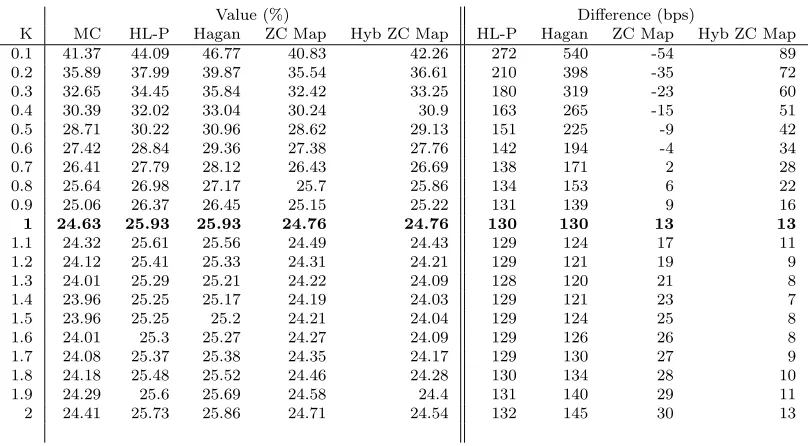
7
Numerical experiments
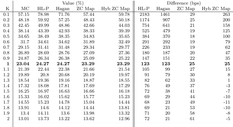
In this section, we demonstrate the efficiency of our approach. We analyze a wide variety of model coefficients for large maturities. The data are summarized in the table below
Rate Initial Value F0 1 SV Initial Value v0 0.25
Vol-of-Vol γ 0.3
Correlations ρ −0.8, −0.5, −0.2 Skews β 0.3, 0.6, 0.9
We present the Black-Scholes implied volatility for European call optionsC(T, K) =E[(FT−K)+] for
a large range of strikesK and as well as second-moment underlying CMS calculations.
CMS convexity adjustments depend on the second moment of the rate process, which can be evaluated by the usual static replication formula (Hagan (2003))
E
FT2
= 2
Z ∞
0
dKE[(FT −K)+]. (7.1)
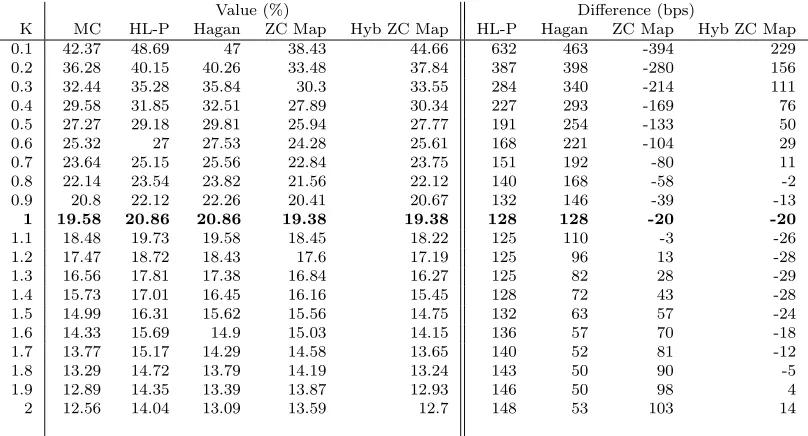
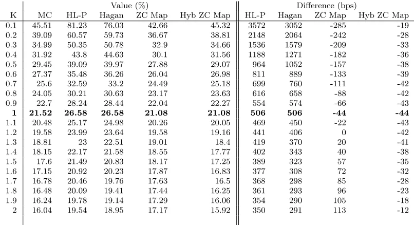
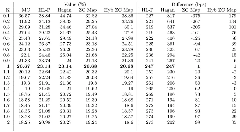
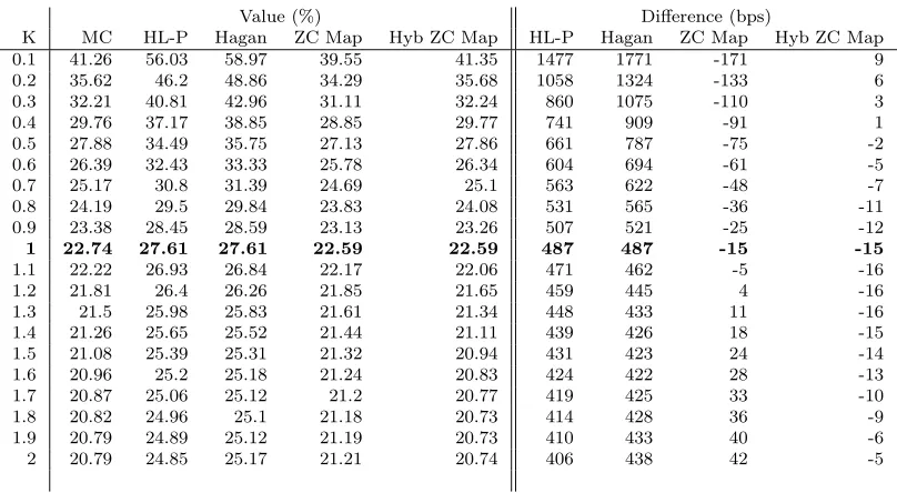
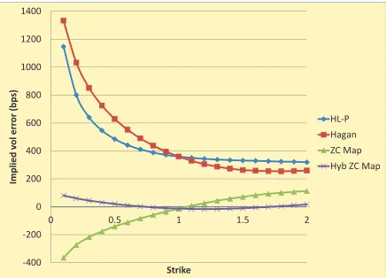
In our numerical experiments, we compare the following methods:
• Monte Carlo simulation (MC)
• The Henry-Labordere (2008) and Paulot (2009) (HL-P) form of the implied volatility expansion (regular leading order and the first correction)
• The Hagan et al. (2002) form of the implied volatility expansion (Hagan)
• Map to the zero correlation SABR model (ZC Map) (regular leading order (2.31) and the first correction (2.32))
Value (%) Difference (bps)
K MC HL-P Hagan ZC Map Hyb ZC Map HL-P Hagan ZC Map Hyb ZC Map 0.1 57.15 78.98 71.76 57.44 59.78 2183 1461 29 263 0.2 48.18 59.92 57.25 48.43 50.18 1174 907 25 200 0.3 42.45 49.99 48.86 42.66 44.03 754 641 21 158 0.4 38.14 43.39 42.93 38.33 39.39 525 479 19 125 0.5 34.65 38.49 38.35 34.83 35.65 384 370 18 100 0.6 31.7 34.61 34.62 31.89 32.49 291 292 19 79 0.7 29.15 31.41 31.48 29.34 29.77 226 233 19 62 0.8 26.89 28.69 28.76 27.09 27.36 180 187 20 47 0.9 24.87 26.34 26.38 25.09 25.22 147 151 22 35
1 23.04 24.27 24.27 23.29 23.29 123 123 25 25
[image:28.595.97.501.140.363.2]1.1 21.39 22.44 22.38 21.66 21.54 105 99 27 15 1.2 19.89 20.8 20.68 20.19 19.97 91 79 30 8 1.3 18.54 19.36 19.16 18.87 18.55 82 62 33 1 1.4 17.32 18.08 17.81 17.69 17.29 76 49 37 -3 1.5 16.25 16.97 16.63 16.66 16.18 72 38 41 -7 1.6 15.33 16.02 15.62 15.77 15.23 69 29 44 -10 1.7 14.55 15.23 14.78 15.04 14.44 68 23 49 -11 1.8 13.91 14.6 14.12 14.44 13.81 69 21 53 -10 1.9 13.4 14.11 13.6 13.98 13.32 71 20 58 -8 2 13.01 13.73 13.22 13.62 12.96 72 21 61 -5
Table 1: Implied vol and its error for different methods, 10Y maturity,
β
= 0
.
3,
ρ
=
−
0
.
8.
Value (%) Difference (bps)
K MC HL-P Hagan ZC Map Hyb ZC Map HL-P Hagan ZC Map Hyb ZC Map 0.1 51.23 56.44 55.18 51.14 54.91 521 395 -9 368 0.2 43.22 46.25 46.15 43.25 45.83 303 293 3 261 0.3 38.27 40.37 40.59 38.35 40.24 210 232 8 197 0.4 34.63 36.22 36.52 34.74 36.14 159 189 11 151 0.5 31.73 33 33.3 31.87 32.89 127 157 14 116 0.6 29.3 30.36 30.62 29.46 30.2 106 132 16 90 0.7 27.22 28.12 28.32 27.39 27.89 90 110 17 67 0.8 25.39 26.17 26.31 25.58 25.88 78 92 19 49 0.9 23.76 24.46 24.53 23.97 24.11 70 77 21 35
1 22.29 22.93 22.93 22.52 22.52 64 64 23 23
1.1 20.96 21.56 21.49 21.21 21.09 60 53 25 13 1.2 19.76 20.33 20.18 20.03 19.82 57 42 27 6 1.3 18.67 19.22 19.01 18.97 18.67 55 34 30 0 1.4 17.7 18.24 17.96 18.02 17.66 54 26 32 -4 1.5 16.83 17.37 17.03 17.19 16.77 54 20 36 -6 1.6 16.07 16.62 16.22 16.46 16 55 15 39 -7 1.7 15.42 15.98 15.54 15.84 15.36 56 12 42 -6 1.8 14.87 15.45 14.98 15.32 14.84 58 11 45 -3 1.9 14.43 15.01 14.54 14.9 14.42 58 11 47 -1 2 14.07 14.66 14.19 14.56 14.11 59 12 49 4
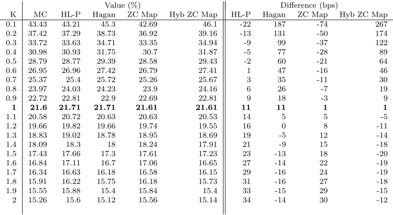
[image:28.595.97.500.142.361.2]Value (%) Difference (bps)
K MC HL-P Hagan ZC Map Hyb ZC Map HL-P Hagan ZC Map Hyb ZC Map 0.1 43.43 43.21 45.3 42.69 46.1 -22 187 -74 267 0.2 37.42 37.29 38.73 36.92 39.16 -13 131 -50 174 0.3 33.72 33.63 34.71 33.35 34.94 -9 99 -37 122 0.4 30.98 30.93 31.75 30.7 31.87 -5 77 -28 89 0.5 28.79 28.77 29.39 28.58 29.43 -2 60 -21 64 0.6 26.95 26.96 27.42 26.79 27.41 1 47 -16 46 0.7 25.37 25.4 25.72 25.26 25.67 3 35 -11 30 0.8 23.97 24.03 24.23 23.9 24.16 6 26 -7 19 0.9 22.72 22.81 22.9 22.69 22.81 9 18 -3 9
1 21.6 21.71 21.71 21.61 21.61 11 11 1 1
[image:29.595.100.499.141.362.2]1.1 20.58 20.72 20.63 20.63 20.53 14 5 5 -5 1.2 19.66 19.82 19.66 19.74 19.55 16 0 8 -11 1.3 18.83 19.02 18.78 18.95 18.69 19 -5 12 -14 1.4 18.09 18.3 18 18.24 17.91 21 -9 15 -18 1.5 17.43 17.66 17.3 17.61 17.23 23 -13 18 -20 1.6 16.84 17.11 16.7 17.06 16.65 27 -14 22 -19 1.7 16.34 16.63 16.18 16.58 16.15 29 -16 24 -19 1.8 15.91 16.22 15.75 16.18 15.73 31 -16 27 -18 1.9 15.55 15.88 15.4 15.84 15.4 33 -15 29 -15 2 15.26 15.6 15.12 15.56 15.14 34 -14 30 -12
Table 3: Implied vol and its error for different methods, 10Y maturity,
β
= 0
.
9,
ρ
=
−
0
.
8.
Value (%) Difference (bps)
K MC Pauloty Hagan ZC Map Hyb ZC Map HL-P Hagan ZC Map Hyb ZC Map 0.1 55.93 76.42 72.71 55.01 56.81 2049 1678 -92 88 0.2 47.12 58.49 57.68 46.39 47.82 1137 1056 -73 70 0.3 41.58 49.13 49.17 41 42.15 755 759 -58 57 0.4 37.48 42.93 43.27 37.02 37.96 545 579 -46 48 0.5 34.22 38.37 38.78 33.86 34.62 415 456 -36 40 0.6 31.52 34.81 35.19 31.25 31.84 329 367 -27 32 0.7 29.24 31.92 32.22 29.05 29.48 268 298 -19 24 0.8 27.27 29.52 29.72 27.17 27.45 225 245 -10 18 0.9 25.56 27.5 27.6 25.54 25.68 194 204 -2 12
1 24.08 25.79 25.79 24.14 24.14 171 171 6 6
1.1 22.8 24.34 24.24 22.93 22.8 154 144 13 0 1.2 21.7 23.11 22.93 21.9 21.65 141 123 20 -5 1.3 20.77 22.08 21.84 21.04 20.67 131 107 27 -10 1.4 19.98 21.23 20.93 20.31 19.86 125 95 33 -12 1.5 19.33 20.53 20.2 19.72 19.18 120 87 39 -15 1.6 18.8 19.96 19.62 19.24 18.64 116 82 44 -16 1.7 18.37 19.51 19.16 18.86 18.21 114 79 49 -16 1.8 18.04 19.16 18.82 18.57 17.88 112 78 53 -16 1.9 17.77 18.88 18.56 18.34 17.63 111 79 57 -14 2 17.57 18.67 18.37 18.16 17.44 110 80 59 -13
[image:29.595.98.499.142.362.2]Value (%) Difference (bps)
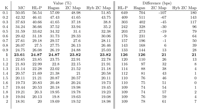
K MC HL-P Hagan ZC Map Hyb ZC Map HL-P Hagan ZC Map Hyb ZC Map 0.1 50.05 56.54 57.09 48.98 51.85 649 704 -107 180 0.2 42.32 46.41 47.43 41.65 43.75 409 511 -67 143 0.3 37.63 40.66 41.65 37.18 38.8 303 402 -45 117 0.4 34.24 36.66 37.52 33.94 35.2 242 328 -30 96 0.5 31.59 33.62 34.32 31.4 32.38 203 273 -19 79 0.6 29.42 31.18 31.73 29.33 30.06 176 231 -9 64 0.7 27.61 29.18 29.57 27.6 28.11 157 196 -1 50 0.8 26.07 27.5 27.75 26.13 26.46 143 168 6 39 0.9 24.75 26.08 26.19 24.88 25.03 133 144 13 28
1 23.61 24.87 24.87 23.82 23.82 126 126 21 21
[image:30.595.96.501.140.363.2]1.1 22.65 23.85 23.75 22.91 22.78 120 110 26 13 1.2 21.83 22.99 22.8 22.15 21.91 116 97 32 8 1.3 21.14 22.28 22.02 21.52 21.18 114 88 38 4 1.4 20.57 21.69 21.38 21 20.58 112 81 43 1 1.5 20.11 21.21 20.87 20.57 20.11 110 76 46 0 1.6 19.73 20.83 20.48 20.24 19.73 110 75 51 0 1.7 19.44 20.53 20.18 19.98 19.45 109 74 54 1 1.8 19.21 20.3 19.95 19.78 19.23 109 74 57 2 1.9 19.04 20.13 19.8 19.63 19.08 109 76 59 4 2 18.91 20 19.69 19.52 18.98 109 78 61 7
Table 5: Implied vol and its error for different methods, 10Y maturity,
β
= 0
.
6,
ρ
=
−
0
.
5.
Value (%) Difference (bps)
K MC HL-P Hagan ZC Map Hyb ZC Map HL-P Hagan ZC Map Hyb ZC Map 0.1 42.56 44.16 47.08 41.52 44.84 160 452 -104 228 0.2 36.81 38.1 40.19 36.18 38.54 129 338 -63 173 0.3 33.32 34.47 36.05 32.91 34.7 115 273 -41 138 0.4 30.81 31.87 33.09 30.55 31.92 106 228 -26 111 0.5 28.85 29.86 30.78 28.71 29.75 101 193 -14 90 0.6 27.27 28.24 28.91 27.22 27.98 97 164 -5 71 0.7 25.95 26.9 27.37 25.99 26.51 95 142 4 56 0.8 24.84 25.78 26.07 24.96 25.28 94 123 12 44 0.9 23.91 24.85 24.98 24.1 24.24 94 107 19 33
1 23.13 24.07 24.07 23.38 23.38 94 94 25 25
[image:30.595.97.498.141.362.2]1.1 22.48 23.42 23.31 22.78 22.66 94 83 30 18 1.2 21.94 22.9 22.69 22.3 22.08 96 75 36 14 1.3 21.5 22.47 22.2 21.91 21.62 97 70 41 12 1.4 21.16 22.14 21.81 21.6 21.26 98 65 44 10 1.5 20.89 21.88 21.51 21.37 20.99 99 62 48 10 1.6 20.68 21.68 21.3 21.19 20.8 100 62 51 12 1.7 20.54 21.55 21.15 21.07 20.68 101 61 53 14 1.8 20.44 21.45 21.07 20.99 20.6 101 63 55 16 1.9 20.37 21.4 21.02 20.94 20.57 103 65 57 20 2 20.35 21.37 21.02 20.93 20.58 102 67 58 23
Value (%) Difference (bps)
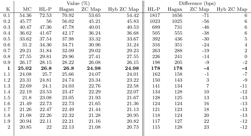
K MC HL-P Hagan ZC Map Hyb ZC Map HL-P Hagan ZC Map Hyb ZC Map 0.1 54.36 72.53 70.92 53.65 54.42 1817 1656 -71 6 0.2 45.77 56 56.02 45.21 45.83 1023 1025 -56 6 0.3 40.47 47.36 47.78 40.01 40.53 689 731 -46 6 0.4 36.62 41.67 42.17 36.24 36.68 505 555 -38 6 0.5 33.62 37.54 37.98 33.32 33.67 392 436 -30 5 0.6 31.2 34.36 34.71 30.96 31.24 316 351 -24 4 0.7 29.21 31.84 32.09 29.02 29.23 263 288 -19 2 0.8 27.55 29.81 29.96 27.41 27.55 226 241 -14 0 0.9 26.17 28.15 28.22 26.08 26.15 198 205 -9 -2
1 25.02 26.8 26.8 24.98 24.98 178 178 -4 -4
[image:31.595.98.501.140.362.2]1.1 24.08 25.7 25.66 24.07 24.01 162 158 -1 -7 1.2 23.31 24.81 24.74 23.34 23.22 150 143 3 -9 1.3 22.69 24.1 24.03 22.76 22.58 141 134 7 -11 1.4 22.19 23.53 23.47 22.29 22.07 134 128 10 -12 1.5 21.8 23.08 23.05 21.93 21.67 128 125 13 -13 1.6 21.49 22.73 22.73 21.65 21.36 124 124 16 -13 1.7 21.26 22.47 22.49 21.44 21.13 121 123 18 -13 1.8 21.08 22.26 22.32 21.28 20.95 118 124 20 -13 1.9 20.94 22.11 22.21 21.16 20.82 117 127 22 -12 2 20.85 22 22.13 21.08 20.73 115 128 23 -12
Table 7: Implied vol and its error for different methods, 10Y maturity,
β
= 0
.
3,
ρ
=
−
0
.
2.
Value (%) Difference (bps)
K MC HL-P Hagan ZC Map Hyb ZC Map HL-P Hagan ZC Map Hyb ZC Map 0.1 48.5 55.39 56.52 47.84 49.03 689 802 -66 53 0.2 41.12 45.53 46.74 40.67 41.57 441 562 -45 45 0.3 36.72 40.03 41.06 36.39 37.11 331 434 -33 39 0.4 33.6 36.28 37.1 33.36 33.94 268 350 -24 34 0.5 31.23 33.5 34.13 31.06 31.51 227 290 -17 28 0.6 29.36 31.35 31.79 29.24 29.58 199 243 -12 22 0.7 27.85 29.64 29.94 27.78 28.03 179 209 -7 18 0.8 26.62 28.27 28.44 26.6 26.76 165 182 -2 14 0.9 25.64 27.18 27.25 25.66 25.73 154 161 2 9
1 24.84 26.3 26.3 24.9 24.9 146 146 6 6
1.1 24.22 25.61 25.57 24.31 24.25 139 135 9 3 1.2 23.73 25.08 25.01 23.85 23.73 135 128 12 0 1.3 23.35 24.67 24.59 23.51 23.34 132 124 16 -1 1.4 23.07 24.36 24.29 23.25 23.05 129 122 18 -2 1.5 22.87 24.13 24.09 23.07 22.85 126 122 20 -2 1.6 22.73 23.98 23.97 22.95 22.71 125 124 22 -2 1.7 22.64 23.87 23.9 22.88 22.62 123 126 24 -2 1.8 22.59 23.81 23.88 22.84 22.57 122 129 25 -2 1.9 22.57 23.79 23.9 22.83 22.56 122 133 26 -1 2 22.57 23.79 23.94 22.85 22.57 122 137 28 0
[image:31.595.98.500.142.361.2]Value (%) Difference (bps)
K MC HL-P Hagan ZC Map Hyb ZC Map HL-P Hagan ZC Map Hyb ZC Map 0.1 41.37 44.09 46.77 40.83 42.26 272 540 -54 89 0.2 35.89 37.99 39.87 35.54 36.61 210 398 -35 72 0.3 32.65 34.45 35.84 32.42 33.25 180 319 -23 60 0.4 30.39 32.02 33.04 30.24 30.9 163 265 -15 51 0.5 28.71 30.22 30.96 28.62 29.13 151 225 -9 42 0.6 27.42 28.84 29.36 27.38 27.76 142 194 -4 34 0.7 26.41 27.79 28.12 26.43 26.69 138 171 2 28 0.8 25.64 26.98 27.17 25.7 25.86 134 153 6 22 0.9 25.06 26.37 26.45 25.15 25.22 131 139 9 16
1 24.63 25.93 25.93 24.76 24.76 130 130 13 13
[image:32.595.97.501.140.363.2]1.1 24.32 25.61 25.56 24.49 24.43 129 124 17 11 1.2 24.12 25.41 25.33 24.31 24.21 129 121 19 9 1.3 24.01 25.29 25.21 24.22 24.09 128 120 21 8 1.4 23.96 25.25 25.17 24.19 24.03 129 121 23 7 1.5 23.96 25.25 25.2 24.21 24.04 129 124 25 8 1.6 24.01 25.3 25.27 24.27 24.09 129 126 26 8 1.7 24.08 25.37 25.38 24.35 24.17 129 130 27 9 1.8 24.18 25.48 25.52 24.46 24.28 130 134 28 10 1.9 24.29 25.6 25.69 24.58 24.4 131 140 29 11 2 24.41 25.73 25.86 24.71 24.54 132 145 30 13
Table 9: Implied vol and its error for different methods, 10Y maturity,
β
= 0
.
9,
ρ
=
−
0
.
2.
Value (%) Difference (bps)
K MC HL-P Hagan ZC Map Hyb ZC Map HL-P Hagan ZC Map Hyb ZC Map 0.1 46.06 81.19 69.25 43.45 47.05 3513 2319 -261 99 0.2 39.55 59.5 55.07 37.41 40.16 1995 1552 -214 61 0.3 35.34 48.9 47.04 33.52 35.69 1356 1170 -182 35 0.4 32.13 42.12 41.38 30.57 32.28 999 925 -156 15 0.5 29.49 37.21 37.02 28.16 29.5 772 753 -133 1 0.6 27.23 33.4 33.46 26.12 27.13 617 623 -111 -10 0.7 25.24 30.3 30.45 24.34 25.05 506 521 -90 -19 0.8 23.46 27.7 27.85 22.75 23.21 424 439 -71 -25 0.9 21.85 25.48 25.57 21.34 21.56 363 372 -51 -29
1 20.37 23.54 23.54 20.06 20.06 317 317 -31 -31
[image:32.595.97.502.416.636.2]1.1 19.02 21.84 21.72 18.9 18.7 282 270 -12 -32 1.2 17.79 20.34 20.08 17.86 17.47 255 229 7 -32 1.3 16.66 19.01 18.62 16.93 16.36 235 196 27 -30 1.4 15.63 17.86 17.32 16.1 15.37 223 169 47 -26 1.5 14.72 16.86 16.18 15.38 14.5 214 146 66 -22 1.6 13.92 16.02 15.2 14.76 13.75 210 128 84 -17 1.7 13.24 15.31 14.4 14.24 13.13 207 116 100 -11 1.8 12.67 14.74 13.75 13.82 12.63 207 108 115 -4 1.9 12.21 14.28 13.26 13.48 12.24 207 105 127 3 2 11.84 13.92 12.89 13.21 11.96 208 105 137 12
Value (%) Difference (bps)
K MC HL-P Hagan ZC Map Hyb ZC Map HL-P Hagan ZC Map Hyb ZC Map 0.1 42.37 48.69 47 38.43 44.66 632 463 -394 229 0.2 36.28 40.15 40.26 33.48 37.84 387 398 -280 156 0.3 32.44 35.28 35.84 30.3 33.55 284 340 -214 111 0.4 29.58 31.85 32.51 27.89 30.34 227 293 -169 76 0.5 27.27 29.18 29.81 25.94 27.77 191 254 -133 50 0.6 25.32 27 27.53 24.28 25.61 168 221 -104 29 0.7 23.64 25.15 25.56 22.84 23.75 151 192 -80 11 0.8 22.14 23.54 23.82 21.56 22.12 140 168 -58 -2 0.9 20.8 22.12 22.26 20.41 20.67 132 146 -39 -13
1 19.58 20.86 20.86 19.38 19.38 128 128 -20 -20
[image:33.595.97.501.139.357.2]1.1 18.48 19.73 19.58 18.45 18.22 125 110 -3 -26 1.2 17.47 18.72 18.43 17.6 17.19 125 96 13 -28 1.3 16.56 17.81 17.38 16.84 16.27 125 82 28 -29 1.4 15.73 17.01 16.45 16.16 15.45 128 72 43 -28 1.5 14.99 16.31 15.62 15.56 14.75 132 63 57 -24 1.6 14.33 15.69 14.9 15.03 14.15 136 57 70 -18 1.7 13.77 15.17 14.29 14.58 13.65 140 52 81 -12 1.8 13.29 14.72 13.79 14.19 13.24 143 50 90 -5 1.9 12.89 14.35 13.39 13.87 12.93 146 50 98 4 2 12.56 14.04 13.09 13.59 12.7 148 53 103 14
Table 11: Implied vol and its error for different methods, 20Y maturity,
β
= 0
.
6,
ρ
=
−
0
.
8.
Value (%) Difference (bps)
K MC HL-P Hagan ZC Map Hyb ZC Map HL-P Hagan ZC Map Hyb ZC Map 0.1 36.7 33.2 37.42 32.2 38.62 -350 72 -450 192 0.2 31.85 29.36 32.27 28.56 32.83 -249 42 -329 98 0.3 28.84 26.89 29.05 26.21 29.29 -195 21 -263 45 0.4 26.59 25.03 26.66 24.42 26.7 -156 7 -217 11 0.5 24.79 23.51 24.75 22.97 24.65 -128 -4 -182 -14 0.6 23.27 22.22 23.13 21.74 22.95 -105 -14 -153 -32 0.7 21.95 21.1 21.74 20.67 21.49 -85 -21 -128 -46 0.8 20.78 20.1 20.51 19.71 20.22 -68 -27 -107 -56 0.9 19.74 19.21 19.4 18.86 19.1 -53 -34 -88 -64
1 18.8 18.41 18.41 18.1 18.1 -39 -39 -70 -70
[image:33.595.100.499.406.626.2]1.1 17.94 17.69 17.52 17.4 17.2 -25 -42 -54 -74 1.2 17.17 17.04 16.7 16.78 16.41 -13 -47 -39 -76 1.3 16.46 16.45 15.97 16.22 15.7 -1 -49 -24 -76 1.4 15.83 15.93 15.32 15.72 15.07 10 -51 -11 -76 1.5 15.26 15.46 14.74 15.27 14.53 20 -52 1 -73 1.6 14.77 15.05 14.24 14.88 14.06 28 -53 11 -71 1.7 14.33 14.7 13.8 14.54 13.67 37 -53 21 -66 1.8 13.95 14.38 13.44 14.24 13.35 43 -51 29 -60 1.9 13.64 14.11 13.15 13.98 13.1 47 -49 34 -54 2 13.38 13.88 12.92 13.75 12.91 50 -46 37 -47
Value (%) Difference (bps)
K MC HL-P Hagan ZC Map Hyb ZC Map HL-P Hagan ZC Map Hyb ZC Map 0.1 45.51 81.23 76.03 42.66 45.32 3572 3052 -285 -19 0.2 39.09 60.57 59.73 36.67 38.81 2148 2064 -