warwick.ac.uk/lib-publications
Manuscript version: Published Version
The version presented in WRAP is the published version (Version of Record).
Persistent WRAP URL:
http://wrap.warwick.ac.uk/123702
How to cite:
The repository item page linked to above, will contain details on accessing citation guidance
from the publisher.
Copyright and reuse:
The Warwick Research Archive Portal (WRAP) makes this work by researchers of the
University of Warwick available open access under the following conditions.
Copyright © and all moral rights to the version of the paper presented here belong to the
individual author(s) and/or other copyright owners. To the extent reasonable and
practicable the material made available in WRAP has been checked for eligibility before
being made available.
Copies of full items can be used for personal research or study, educational, or not-for-profit
purposes without prior permission or charge. Provided that the authors, title and full
bibliographic details are credited, a hyperlink and/or URL is given for the original metadata
page and the content is not changed in any way.
Publisher’s statement:
Please refer to the repository item page, publisher’s statement section, for further
information.
Efficient Bayesian Model Choice for Partially
Observed Processes: With Application to an
Experimental Transmission Study of an
Infectious Disease
Trevelyan J. McKinley∗, Peter Neal†, Simon E. F. Spencer‡, Andrew J. K. Conlan§, and Laurence Tiley§
Abstract. Infectious diseases such as avian influenza pose a global threat to hu-man health. Mathematical and statistical models can provide key insights into the mechanisms that underlie the spread and persistence of infectious diseases, though their utility is linked to the ability to adequately calibrate these models to observed data. Performing robust inference for these systems is challenging. The fact that the underlying models exhibit complex non-linear dynamics, coupled with prac-tical constraints to observing key epidemiological events such as transmission, requires the use of inference techniques that are able to numerically integrate over multiple hidden states and/or infer missing information. Simulation-based infer-ence techniques such as Approximate Bayesian Computation (ABC) have shown great promise in this area, since they rely on the development of suitable simu-lation models, which are often easier to code and generalise than routines that require evaluations of an intractable likelihood function. In this manuscript we make some contributions towards improving the efficiency of ABC-based particle Markov chain Monte Carlo methods, and show the utility of these approaches for performing both model inference and model comparison in a Bayesian frame-work. We illustrate these approaches on both simulated data, as well as real data from an experimental transmission study of highly pathogenic avian influenza in genetically modified chickens.
Keywords:Bayesian model choice, infectious disease models, partially observed processes, particle MCMC, Approximate Bayesian Computation.
1
Introduction
Infectious diseases such as avian influenza pose a global threat to human health. Mathe-matical modelling can elucidate on key mechanisms that underlie disease spread, which can directly inform the control of potential outbreaks. However, the utility of these approaches depends greatly on the ability to calibrate them to observed data. For
ex-∗College of Engineering, Mathematics and Physical Sciences, University of Exeter, Penryn, UK, [email protected]
†Department of Mathematics and Statistics, Lancaster University, Lancaster, UK
‡Department of Statistics and the Warwick Analytical Sciences Centre, University of Warwick, Coventry, UK
§Department of Veterinary Medicine, University of Cambridge, Cambridge, UK
c
Figure 1: Data taken from Lyall et al. (2011).
Experiment Exposure Genotype Number of birds
1 In-contact NTG 12
Challenge 5
2 In-contact TG 12
Challenge NTG 5
3 In-contact NTG 12
Challenge TG 5
4 In-contact TG 12
Challenge 5
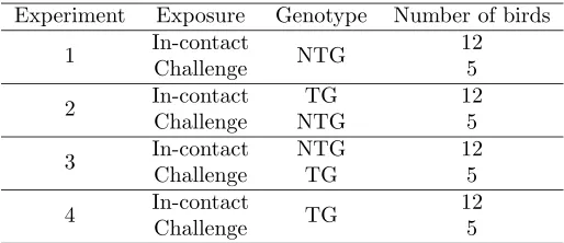
Table 1: Experimental conditions (from Lyall et al.,2011).
ample, Lyall et al. (2011) genetically modified chickens to be resistant to avian influenza. Thesetransgenic chickens expressed a short-hairpin RNA designed to function as a de-coy, and hence interfere and hinder viral propagation. In order to assess the efficiacy of the modification they ran a series of natural transmission experiments. They used a crossed experimental design in which four experiments were undertaken, where each experiment used 5 challenge birds (that had been inoculated with highly pathogenic avian influenza—HPAI) co-housed with 12 uninfected in-contact birds. Each experi-ment was run over 10 days, with each bird being swabbed twice daily (producing buccal and cloacal swabs). Some birds were artificially removed from the study (if they were clinically sick, or sometimes for other blood work to be done), some birds died naturally, and others were euthanased at the end of the study. From these data it is possible to derive integer-valued time series counts for the number of infections for each genotype over each half-day period, which are shown in Figure1.
[image:3.612.177.434.326.437.2]exper-iments where the transgenic (TG) birds constituted the challenge group. In Lyall et al. (2011) these differences were compared using a series of Bonferroni corrected Mann-Whitney tests. However, a key question that remained was whether these patterns could be caused by differences in transmission potential between the genotypes, differences in susceptibility to infection, or both. The supposition in Lyall et al. (2011) was that it was the former, but the crude Mann-Whitney test is not sufficient to provide evidence for or against these competing hypotheses. In this paper we develop a framework to estimate the Bayesian evidence (e.g. Kass and Raftery, 1995) for a series of competing dynamic transmission models that allows us to directly address these questions.
2
Statistical methods
Infectious disease systems often have complex non-linear dynamics, which are not well captured by classical statistical approaches to inference, such as generalised linear mod-elling or null hypothesis significance testing. A common way to model these processes is to use compartmental models, where individuals progress through a series of different epidemiological states over time (e.g. Anderson and May,1991). Stochastic versions of these models are parameterised by the average rates of progression through the com-partments, which are dependent on the state of the system at any given time (e.g. Keeling and Rohani,2008).
The main challenge for inference is that even in highly controlled settings it is not possible to directly observe key measurements required to reconstruct a likelihood func-tion, such as the time of infecfunc-tion, or even the infection status of animals (particularly in presence of sub-clinical infections). Hence the problem becomes that of inference for hidden Markov (or non-Markovian) models (HMMs).
The Bayesian paradigm provides a natural framework within which to tackle these problems, since the uncertainties associated with the hidden process are propagated through the system and explicitly incorporated into the parameter estimates and pre-dictions from the model. Here we wish to estimate the posterior distribution for the parameters,θ, given the observed datay, which is in turn dependent on hidden states
x. In this case the posterior,f(θ|y), is defined as:
f(θ|y)∝f(y|θ)f(θ) =
Xf(y,x|θ)dx
f(θ), (1)
whereX corresponds to the sample space for the hidden variablesxandf(θ) is theprior
distribution for the parametersθ. The idea is that by modelling the missing information, the joint distributionf(y,x|θ) has a specific (and known) mathematical form.
Andrieu and Roberts, 2009; Andrieu et al., 2010). Under certain conditions, Andrieu and Roberts (2009) showed that as long as the estimate of the likelihood is unbiased
andnon-negative, then a Markov chain Monte Carlo (MCMC; see e.g. Gilks et al.,1996) algorithm can be developed that produces samples from the correct posterior distribu-tion in probability (see also Beaumont,2003). Due to the dynamic nature of infectious disease models, direct simulation is often inefficient, but the structure of the models can often be exploited to produce more efficient estimators. For example, particle filtering methods (see e.g. Doucet et al., 2001) are now often used to produce a non-negative and unbiased likelihood estimate for state-space models, which can have a lower vari-ance than vanilla MC estimators. These hybrid methods are known asparticle MCMC
(PMCMC; e.g. Andrieu et al.,2010; Drovandi et al.,2016; Alzahrani et al.,2018), and are attractive because it is often far easier to code a simulation model than it is to optimise more traditional approaches to dealing with HMMs, such as data-augmented (reversible-jump) MCMC (e.g. Gibson and Renshaw,1998; O’Neill and Roberts, 1999; Jewell et al., 2009). Despite this, PMCMC methods can be highly computationally in-tensive, but in practice they can be made more efficient by introducing a discrepancy function, such that simulations do not have to be exactly consistent with the observed data but rather have to be within some region ‘close’ to the data (e.g. Del Moral et al., 2015; Drovandi et al.,2016). This reduces the computational burden of the routines at the cost of producing an approximate (rather than exact) posterior. Recently Wilkin-son (2013) provides an alternative interpretation of this approximate distribution as the exact posterior distribution for a model incorporating specific model discrepancy (or measurement error) terms.
These latter approaches come under a generic suite of methods known as Approxi-mate Bayesian Computation (ABC; e.g. Tavar´e et al.,1997; Marjoram et al.,2003; Toni et al., 2009; McKinley et al.,2009, 2018), which aim to improve the efficiency of nu-merical estimation algorithms through both dimension reduction techniques (by fitting to summary measures of the data, rather than the full data), in addition to the use of discrepancy measures. However, in this manuscript we place a discrepancy function aroundeach data point, and we do not further approximate by reducing the data to a set ofsummary statistics, which can cause challenges in ABC-based model choice routines (see e.g. Marin et al., 2014; though we note interesting recent work by Pudlo et al., 2016 and Raynal et al., 2017 that aim to perform robust model choice and inference respectively within the classic ABC paradigm using random forests—see e.g. Breiman, 2001). In our case, as the discrepancy tolerance reduces to zero around each data point, the approximate posteriors converge to the exact posterior (with no model discrepancy).
2.1
The alive particle filter
To fit the models we used the particle MCMC algorithm of Drovandi et al. (2016) using the alive particle filter (APF) of Del Moral et al. (2015). From now on we discuss the algorithms in the context of the systems presented in this paper, but note that other generalisations can also be used (e.g. Drovandi et al.,2016).
Consider datay= (y1, . . . ,yT) as a set of integer counts at time pointst= 1, . . . , T.
data yt = (y1t, . . . , yGt) where G ≥ 1. We also introduce a fixed set of tolerances,
={t; fort= 1, . . . , T}, where t={gt; forg= 1, . . . , G}.
We can then condition the likelihood,f(y|θ), on the tolerances, and write this as:
f(y|,θ) =
X[f(y,x|θ)]dx,
=
X
fX0(x0|θ) T
t=1
fYt|Xt(yt|xt,t)fXt|Xt−1(xt|xt−1,θ)
dx, (2)
wherefX0(x0|θ) is the density function for the initial conditions for the hidden states at time 0 (which may or may not depend on the unknown parametersθ). The density
fXt|Xt−1(xt|xt−1,θ) governs the progression from state xt−1 to state xt based on the underlying model, and fYt|Xt(yt|xt,t) is the discrepancy/observation term for
the data yt conditional on the hidden states xtand the tolerances t. The integral in
(2) is now over the multidimensional space X corresponding to all possible values for the hidden states xt at time points t = 0, . . . , T. In this manuscript, we consider the
discrepancy term,f(yt|xt,t), to be an indicator function, such that
f(yt|xt,t) = G
g=1
fYgt|Xgt(ygt|xgt, gt), (3)
and
fYgt|Xgt(ygt|xgt, gt) =
1 if|hg(xgt)−ygt| ≤gt,
0 otherwise. (4)
Herehg(·) corresponds to a deterministic function mapping the hidden statesxgtto the
same scale as the observed dataygt(e.g. collapsing continuous event times to counts of
events in the period (t−1, t]). (We note that xgt might be of higher dimension than
ygt, and thushg(·) might involve reducing the dimensionality ofxgt, hence the slightly
unwieldy notation.) The tolerances, gt, define how closely we require the transformed
hidden states hg(xgt) to match the data ygt. As gt → 0 for all g and t, then the
transformed hidden states are required to match the data exactly.
Particle filtering techniques aim to approximate (2) by using a finite set of parti-cles, each corresponding to a particular realisation of the hidden states. In this context we could implement a classic bootstrap particle filter (Gordon et al., 1993), such that
N particles are initialised by drawing independently from fX0(x0|θ) and then prop-agated over time by simulating from the underlying model—with probability density
fXt|Xt−1(xt|xt−1,θ)—and weighting each particle according to the discrepancy func-tion fYt|Xt,t(yt|xt, t). There are various straightforward ways to simulate from the
kinds of stochastic compartmental models being studied in this paper, such as Gillespie’s algorithm (Gillespie,1977), and thus in the ABC setting described above, the problem can be reduced to simulating from the underlying model and recording whether the simulation is consistent with the data according to the discrepancy function.
Algorithm 1Alive Particle Filter.
Require: Number of particlesN, parametersθ, and tolerancest, fort= 1, . . . , T.
1: Initialise the log of the estimated likelihood: log fˆ(y|,θ)
=Tlog(N).
2: fort= 1, . . . , T do
3: Setnt= 0.
4: forn= 1, . . . , N + 1do
5: Setδ= 0.
6: while δ= 0do
7: if t= 1then
8: Setr=nand sample initial statesxr
0from fX0(· |θ).
9: else
10: Sample an index runiformly from the set{1, . . . , N}.
11: end if
12: SimulatextfromfXt|Xt−1
· |xrt−1,θ.
13: Setnt=nt+ 1.
14: if fYt|Xt(yt|xt,t) = 1then 15: Setxnt =xtandδ= 1. 16: end if
17: end while
18: end for
19: Set log fˆ(y|,θ)
= log fˆ(y|,θ)
−log (nt−1).
20: end for
estimates. This is keenly felt when the discrepancy function produces binary weights, in which case it is possible to end up with all particles having exactly zero weight. Various extensions to the bootstrap particle filter have been proposed that aim to try to mediate these challenges, and the reader is encouraged to see e.g. Doucet et al. (2001) and Doucet and Johansen (2011) for comprehensive overviews of particle filtering techniques. Recently, Del Moral et al. (2015) proposed thealive particle filter (APF) as a means of tackling this problem for binary weights. The APF continuously resamples particles at each time point untilNparticles with non-zero weights have been obtained. This potentially solves the particle degradation problem, at the cost of making the number of simulations a random variable with a theoretically infinite range. In practice the filter can be stopped after a pre-defined number of simulations has been exceeded, improving the efficiency of particle MCMC algorithms at the cost of some bias in the estimated posteriors (see Drovandi et al.,2016). We return to this problem in Section4.
The APF is outlined in Algorithm1. The estimated likelihood (integrating over the hidden states) is
ˆ
f(y|,θ) =
T
t=1
N nt−1
, (5)
where N is the number of particles, and nt is the number of simulations from the
underlying model required to obtain N+ 1 matches in the period (t−1, t] (thismust
Algorithm 2ABC pseudo-marginal Metropolis-Hastings (ABC-PMMH) algorithm. As
→0then the algorithm converges to the true posterior in probability. Require: Number of iterationsM and tolerances.
1: Initialise parameters θ(0) and calculate an unbiased, non-negative estimate of the likelihood ˆfy|,θ(0).
2: fori= 1, . . . , M do
3: Propose candidate parametersθ from some proposal distributionq(·) (here we use a random-walk proposal).
4: Calculate an unbiased, non-negative estimate of the likelihood ˆf(y|,θ).
5: Calculate the acceptance probability:
α= min
1, fˆ(y|,θ )
ˆ
fy|,θ(i−1)×
f(θ)
fθ(i−1)×
qθ(i−1)|θ
qθ |θ(i−1)
.
6: Sampleu∼U(0,1).
7: if u < αthen
8: Setθ(i)=θ.
9: else
10: Setθ(i)=θ(i−1).
11: end if
12: end for
Andrieu and Roberts (2009) showed that substituting an unbiased, non-negative
estimate of f(y|θ) into a standard Metropolis-Hastings algorithm (Metropolis et al., 1953; Hastings,1970) will produce samples from the exact posterior in probability. This general pseudo-marginal Metropolis-Hastings algorithm is shown in Algorithm 2, and following Del Moral et al. (2015) and Drovandi et al. (2016) we use the APF to produce a suitable unbiased estimate ˆf(y|θ). We will refer to Algorithm2as the ABC-PMMH algorithm.
2.2
Bayesian model choice
The ABC-PMMH algorithm provides a straightforward way to produce estimates of the (approximate) posterior distribution in the presence of hidden states. However, it is also often the case that there are various different ways in which the dynamics of the system could be modelled, which could lead to a very different understanding of how the underlying processes operate. Weighting the degree-of-evidence in favour of different competing models can help to elucidate some of these key mechanisms.
Bayesian model choice is frequently built around the concept of Bayes’ Factors and posterior probabilities of association (Jeffreys,1935,1961). Formally, if we haveW com-peting models to choose from—denoted M1, . . . , MW—then we can derive a posterior
probability for modelMw as
P(Mw|y) =
f(y|Mw)P(Mw)
W
l=1f(y|Ml)P(Ml)
where P(Mw) is the prior probability for model Mw. We note that this is not an
absolute measure of model adequacy, rather it provides a relative posterior weighting conditional on the choice ofW models. However, assuming no uncertainty in the choice of model can often lead to over-confident inferences (e.g. Kass and Raftery,1995; Hoet-ing et al.,1999), and techniques such as such Bayesian Model Averaging (BMA), where applicable, can use these posterior weightings to help to improve the robustness of model predictions. The reader is referred to Kass and Raftery (1995) and Hoeting et al. (1999) for comprehensive introductions to these techniques.
Alternative Bayesian model choice approaches include the Deviance Information Cri-terion (DIC; Spiegelhalter et al.,2002), and posterior predictive p-values (e.g. Gelman et al.,2013). The former provides a Bayesian analogy to the popular Akaike’s Informa-tion Criterion (AIC; Akaike,1974), and is attractive because it can be easily calculated directly using posterior samples. It does not provide a probabilistic weight associated with each model, and thus cannot be used for model averaging, and is most useful for choosing between nested models. Posterior predictive p-values are a useful tool that can be used effectively to assess goodness-of-fit of competing models, which can then be used to inform model choice. The idea is to set up a loss function, which is eval-uated over a set of posterior predictive samples to generate a measure of discrepancy against a pre-specified ideal scenario. An effective use of this approach is given in Lau et al. (2014), in which posterior predictive p-values are used to inform on the validity of different choices of distance kernel for a spatially explicit infectious disease model. However, as with DIC, these approaches do not provide a relative probabilistic weight, and thus cannot be used for model averaging.
As such, the focus of this manuscript is to estimate Bayes’ Factors, and by extension posterior probabilities of association. The key quantity that underpins these ideas is the
marginal likelihood:
f(y|Mw) =
Θw
f(y|θw, Mw)f(θw|Mw)dθw, (7)
where the integral is over the (multidimensional) parameter space for modelMwdenoted
byΘw. The marginal likelihood is equivalent to the normalising constant in (1) and is
often referred to as the Bayesian evidence. In contrast to many frequentist quantities for weighting models, such as AIC, the Bayesian evidence marginalises (rather than maximises) over the parameter space. This means that uncertainties due to hidden states or auxiliary variables are explicitly incorporated into the Bayesian evidence, and that Bayes’ Factor based model choice techniques are naturally parsimonious.
These techniques involve a two-stage process: firstly each competing model is fitted to the data using some numerical algorithm, such as MCMC, and then an approximation to the posterior distribution is used as an importance sampling distribution for estimating (7). To start with, consider that in the presence of hidden states the marginal likelihood for an arbitrary model (dropping the model index for brevity) can be written:
f(y|) =
Θ
X
f(y|x,)f(x|θ)f(θ)dxdθ. (8)
Under the paradigm of Wilkinson (2013), as → 0then the true marginal likelihood (for a model with no model discrepancy) is recovered. Drovandi et al. (2016) suggest approximating (8) as
ˆ
f(y|) = 1
R
R
r=1 ˆ
f(y|θr)f(θr)
q(θr)
, (9)
where the θr are sampled from a distribution with probability density function q(·),
which is an approximation to the posterior distribution f(θ|y) and can be obtained by fitting an auxiliary distribution to the posterior samples obtained from the ABC-PMMH algorithm. Tran et al. (2013) show that (9) produces an unbiased estimate of
f(y|), and for a givenθr, the estimate ˆf(y|θr) can be calculated using the APF
(see also Touloupou et al.,2018; Alzahrani et al.,2018).
3
Data and model structures
The full data for the four experimental settings—as a set of time-series counts (and ignoring the swab information)—are shown in Figure1. The initial experimental condi-tions are summarised in Table 1. We assume that all deaths are recorded at the end of each half-day period. We do not observe infection times, and so have removal information only. For simplicity we assume that culled moribund birds would have died naturally before the end of the corresponding time period in which they were euthanased (and are thus treated as natural removals within a given half-day period). We note that there are also healthy birds that were killed for immunohistological studies, which correspond to censored animals.
We will assume the system follows a stochastic, homogeneously mixing, frequency-dependent SIR model, in a closed population of size N. Hence at any point in time birds are eithersusceptible (S),infected and infectious (I), orremoved (dead;R). We use superscripts to denote genotype, such that for a given experimental setting, there areNT Gtransgenic birds and NN T Gnon-transgenic birds (with total number of birds
N =NT G+NN T G). We define a range of models, with the simplest model assuming that all challenge birds are infected on inoculation with probability p, and that there are no differences in either susceptibility to infection or onward transmission of infection between the genotypes. In this case we can characterise the probability of S → I or
I→R moves in some small time interval (t, t+dt) as:
P(S→I in (t, t+δt)) = βSI
N dt+o(dt), P(I→R in (t, t+δt)) =γIdt+o(dt),
where I=IT G+IN T G is the total number of infected birds, S=ST G+SN T G is the total number of susceptible birds and N = S+I is the total number of birds in the cage. Hereβ is thetransmission parameter, andγis the removal rate(hence 1/γ is the mean infectious period).
We can extend this model in various ways. Firstly, we could assume that the proba-bility of infection post-inoculation varies between genotypes (e.g. with probaproba-bilitypT G
andpN T Gfor the transgenic and non-transgenic birds respectively). We can also allow
for different transmission terms (βT GandβN T G), different susceptibility terms
(param-eterised such that νT G = 1 and νN T G = 1), and/or different removal rates (γT G and
γN T G). Hence the most complex model is characterised by:
PSN T G→IN T Gat time 0∼BinSN T G, pN T G,
PST G→IT G at time 0∼BinST G, pT G,
PSN T G→IN T G in (t, t+δt)=ν
N T GSN T G
N
βT GIT G+βN T GIN T Gdt+o(dt),
PIN T G→RN T G in (t, t+δt)=γN T GIN T Gdt+o(dt),
PST G→IT G in (t, t+δt)=S
T G
N
βT GIT G+βN T GIN T Gdt+o(dt),
PIT G→RT G in (t, t+δt)=γT GIT Gdt+o(dt).
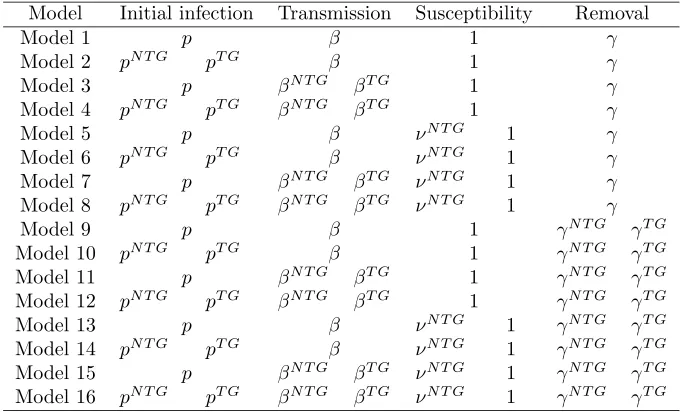
(11) The full list of models considered are characterised in Table2.
In this particular situation we have four independent experiments, and thus we can run the APF for each data set in turn, with an unbiased estimator of the likelihood being given by:
ˆ
f(y|θ,) =
K
k=1
Tk
t=1
Nk
nkt−1
, (12)
wherek= 1, . . . , K denotes the data sets (withK= 4 here),Nkis the number of
parti-cles used in thekthparticle filter, andn
ktis the number of simulations required to obtain
Nk+ 1 matches in time period (t−1, t]. Since there are two different genotypes (NTG
and TG birds), the different experiments have different numbers of removal curves. Experiments 1 and 4 have a single curve each (for NTG and TG birds respectively), whereas experiments 2 and 3 both have two removal curves—one for each genotype. (In the parlance of Section2.1, we have thatG= 1 for experiments 1 and 4, andG= 2 for experiments 2 and 3.) We simplify matters by choosing a common tolerance,across all time-points and all curves. Therefore in experiments 1 and 4 a ‘match’ is obtained if the simulated number of removals matches the data shown in Figure1, whereas for experi-ments 2 and 3 a ‘match’ is obtained if the simulated number of removals forboth geno-types matches each corresponding curve in Figure1 simultaneously—see equation (3).
Data augmentation and censoring
Model Initial infection Transmission Susceptibility Removal
Model 1 p β 1 γ
Model 2 pN T G pT G β 1 γ
Model 3 p βN T G βT G 1 γ
Model 4 pN T G pT G βN T G βT G 1 γ
Model 5 p β νN T G 1 γ
Model 6 pN T G pT G β νN T G 1 γ
Model 7 p βN T G βT G νN T G 1 γ
Model 8 pN T G pT G βN T G βT G νN T G 1 γ
Model 9 p β 1 γN T G γT G
Model 10 pN T G pT G β 1 γN T G γT G
Model 11 p βN T G βT G 1 γN T G γT G
Model 12 pN T G pT G βN T G βT G 1 γN T G γT G
Model 13 p β νN T G 1 γN T G γT G
Model 14 pN T G pT G β νN T G 1 γN T G γT G
Model 15 p βN T G βT G νN T G 1 γN T G γT G
[image:12.612.135.479.120.326.2]Model 16 pN T G pT G βN T G βT G νN T G 1 γN T G γT G
Table 2: Competing model specifications. Model 1 corresponds to the model defined in equation (10), where there are no differences between NTG and TG birds. Model 16 corresponds to the model defined in equation (11), where each component of the model (probability of infection following challenge, transmission, susceptibility and recovery) differ between NTG and TG birds. Intermediate models can be derived by equating different components between the genotypes (e.g. Model 15 can be derived from Model 16 by settingpN T G=pT G=pand so on).
have non-zero weight at a time pointt, but will never produce particles with non-zero weights at time points > t. This can happen, for example, if the number of infectives is zero at time t, but there are additional infections at a time point t∗ > t. In the
SIRframework, the probability of any further infection events is zero if the number of infectives I = 0. In this manuscript, we follow the approach of Drovandi et al. (2016) and augment the data at each time point to include the information regarding whether further infections happen at later time points. For = 0, then this is equivalent to requiring thatIt>0 at time pointtif there are additional infections at later time points.
For >0 we require that It >0 if the cumulative number of infections CtI < NI−,
whereNI is the maximum number of infections observed in the data. Simulations that
do not adhere to these constraints are rejected. We only built in information on censoring for exact matching, at which point we randomly removed an animal at the end of the corresponding time period, and before the matching criteria was employed.
4
Improving the efficiency of the APF in ABC-PMMH
algorithms
thus could result in a huge computational burden, particularly since the filter needs to be run for a large number of MCMC iterations. This is further compounded when esti-mating the marginal likelihood where many more evaluations of the APF are required. Finally we must repeat this process for multiple models. However, in development terms the ABC-PMMH approach is attractive, since the method is fairly straightforward to code and adapt to different models. Therefore methods for improving the efficiency of the APF in the context of ABC-PMMH can help to alleviate the computational burden of the models and increase the size and complexities of systems that can be modelled using this technology.
One way to stop excessive runtimes in the APF is to put a cap on the total number of simulations that the filter is allowed to evaluate (see Drovandi et al.,2016). Therefore if, at some time pointj≤T,
j
t=1
nt> Ns, (13)
then the estimate ˆf(y|θ) is set to 0, where Ns is some arbitrary (large) integer. If
implemented in an ABC-PMMH routine, then this would result in proposals being automatically rejected if the total number of simulations exceeds Ns. This introduces
bias into the estimated posterior distribution, but the bias will decrease as Ns→ ∞.
Thus choosing a suitable value forNsis a trade-off between efficiency and bias; it needs
to be large enough that few proposals result in Ns being exceeded, but small enough
that it doesn’t result in excessively long runtimes. In small systems this may not be an issue, but in larger systems, especially in poor regions of parameter space, or for a poorly specified model, then this can have much more of an impact on the efficiency of the ABC-PMMH routine. (Note that since the filtering is done over different time points, we define the total number of ‘simulations’ to aggregate over the time points, rather than a single simulation being a single realisation across all time points.)
We term the proportion of iterations where the proposal is rejected due to the particle filter failing to complete within Ns simulations (i.e. failing the criteria in 13) as the skip rate. A major challenge is that as the tolerances get small, the skip rate naturally increases, and this will induce more bias in the estimated posterior unless
Nsis also increased. We now introduce an idea that aims to mediate this problem, by
noting that it is possible to reject proposals without necessarily having to evaluate the APF to completion. This reduces both the computational load of the standard APF and the bias introduced by the cut-offNs.
To formulate this idea, consider that at a given iteration i of the ABC-PMMH algorithm (Algorithm2), we accept a proposal,θ, with probability:
α= min
1,
ˆ
f(y|,θ)f(θ)qθ(i)|θ ˆ
fy|,θ(i)fθ(i)qθ|θ(i)
. (14)
Computationally, this is equivalent to simulating a random numberu∼U(0,1), and then acceptingθifu < α. Usually we calculate ˆf(y|,θ), and thusαbefore we simu-lateu. However, sinceuis independent ofα, there is no reason why we cannot simulate
rejectθ if:
u >
ˆ
f(y|,θ)f(θ)qθ(i)|θ
ˆ
fy|,θ(i)fθ(i)qθ|θ(i)
⇐⇒ log fˆ(y|,θ)
< log(u)−A(i), (15)
whereA(i)= log[f(θ)q(θ(i)|θ)]−log[ ˆf(y|,θ(i))f(θ(i))q(θ|θ(i))]. From (5) we can re-write the inequality (15) as
T
t=1
log (nt−1)> Tlog(N)−log(u) +A(i). (16)
Now the only unknown is on the left-hand side of equation (16), and this is a monoton-ically increasing function with respect tont, where the sum must be conducted in order
from t= 1, . . . , T. Hence, for some time pointj ≤T, ifnj reaches a point such that
log (nj−1)> Tlog(N)−log(u) +A(i)−
j−1
t=1
log (nt−1)
, (17)
then the proposal can be rejected with no loss-of-information. This places a finite upper bound on the number of simulations required to reject the proposal that depends only on the previous iteration and the simulation of the random variableu. If all time points eval-uate such thatTt=1log(nt−1)< Tlog(N)−log(u)+A(i)then the proposal is accepted.
We note that this idea to swap the order of evaluations in MCMC accept-reject steps has been employed before in other contexts, notably Beskos et al. (2006) and Pa-paspiliopoulos and Roberts (2008), who employed a similar approach in diffusion pro-cesses and Dirichlet propro-cesses respectively, to evaluate an infinite dimensional function in finite time. They termed their approaches “retrospective sampling”. More recently, Solo-nen et al. (2012) used these ideas when evaluating the likelihood function in complex climate models, and termed their approach “early rejection sampling”. This was ex-tended into the ABC framework by Picchini (2014). Similar ideas of early stopping of simulations were used in early ABC papers such as McKinley et al. (2009), though these did not invert the accept-reject step, but exploited the evaluation of specific non-decreasing summary measures to stop simulations once it was known that it would be rejected. There are also links to ideas of squeezing approaches to rejection sampling (see e.g. Devroye,1986), in the sense of rejecting proposals without having to evaluate com-plex functions to completion. However, these ideas have not been employed on the APF, and are important since the evaluation of the APF could take theoretically infinite time.
each iteration of the MCMC chain, then these approaches can be used to reduce the number of particles needed in order to obtain efficient mixing. Whilst these approaches look promising, we do not explore them further here due to the need to keep track of the random variables used for each simulation, regardless of whether or not the simulation is accepted, which can be prohibitively large. In addition, the correlated methods for updating random variables work best when the observation process is continuous, and in our case this is a binary indicator based on whether the simulations match the observed data according to a pre-defined tolerance. Thus small changes in the non-centred random variables can lead to a previously accepted simulation being rejected or visa-versa, which may affect the performance of the resulting MCMC algorithm.
4.1
Further efficiency savings
We note that for a given time period j, the value of log (nj−1) increases slowly with
respect to increasingnj. For example, for a fixed computational effort,a+bsimulations
say (witha >1 andb >1), then log(a+b)≤log(a) + log(b). Hence it makes sense to split computational effort across multiple time points if possible (since we are summing a set of logged counts), rather than focus on individual time points one at a time (where we are logging a single count). However, since the simulation order cannot be changed in the particle filter, we can instead try an alternative, but related approach, by considering writing (16) as:
j−1
t=1
log (nt−1)
+log (nj−1)+
⎡ ⎣ T
t=j+1
log (nt−1)
⎤
⎦> Tlog(N)−log(u)+A(i). (18)
If we are currently evaluating time point j, then the term in the first set of square brackets in equation (18) has already been calculated. The term in the second set of square brackets in equation (18) has yet to be evaluated and so is ignored in terms of whether we reject the proposal based on the current value of nj. However, we know
that there is a minimum value that the future termsTt=j+1log (nt−1) can take. This
corresponds to every simulation at future time points being accepted first time. Under that scenario,nt=N+1 fort=j+1, . . . , T. Substituting this into (18) and re-arranging
means that at time point j we canreject the proposal if
log (nj−1)> Tlog(N)−log(u) +A(i)−(T−j) log(N)−
j−1
t=1
log (nt−1)
. (19)
The term of the right-hand side of (19) is now smaller than the term of the right-hand side of (17), and thus we have reduced the upper bound onnj.
evaluated is still very high, and hence in practice it is still necessary to place some fixed upper boundNson the total number of simulations to reduce the overall computational
burden. However, in general the proposed approach reduces both the skip rateand the computational load of the algorithms.
In Supplementary Section S1 (McKinley et al., 2019) we discuss additional exten-sions to this idea that worked well for our specific data. The first, which we denote APF∗, extends the ideas outlined above to incorporate the fact that the data come from multiple independent experiments. The second, which we denote APF∗∗ exploits the independence of the different experiments to enable us to split the computational load across the different experiments in order to improve efficiency further.
These approaches only work as part of an MCMC algorithm, and for calculating the marginal likelihood in (9) one has to use the standard APF. We also note that the general idea of simulatingufirst could also be used in other routines, such as PMMH algorithms using the standard bootstrap filter, or even exact MCMC where the computation of the likelihood function is expensive. However, we expect the efficiency savings to be higher in the APF case, since there is greater variability in runtimes of the filter.
4.2
Efficiency of methods
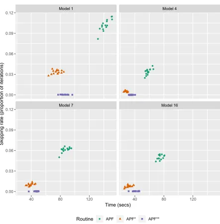
We compare these approaches by fitting four different models (Models 1, 4, 7 and 16 from Table2) to the Avian Influenza Virus (AIV) experimental data in Figure1. We produced 15 runs of the ABC-PMMH algorithm, using the standard APF (with no efficiency adjustments), as well as the APF∗and APF∗∗approaches. Initial values were randomly sampled from the priors in each case, and each run consisted of 10,000 iterations burn-in, followed by a further 10,000 iterations. We used N = 100 particles and a tolerance of = 4 for all data points, with the skip condition Ns set to 2,000×N = 200,000
simulations. The results are shown in Figure 2, and the timings were taken from the final 10,000 iterations (to try to alleviate any bias that might be caused by individual chains being initialised far away from the area of high posterior mass).
We can see that both the APF∗ and APF∗∗ filters have a much lower skip rate in general than the standard APF. This corresponds to shorter run times. We note that the efficiency savings will depend greatly on the computational burden of the simulation model. Here the simulator is fast to evaluate, so the savings are not perhaps as pronounced as they would be for more computationally intensive models. In some cases the APF∗approach was slightly quicker than the APF∗∗ approach, which results from the higher overheads of the APF∗∗approach switching between the different time-series. However, we note that these differences are not large, and furthermore the APF∗∗ routine has a negligible skip rate in nearly all cases (for these settings), and so we think this represents the optimal option going forwards.
4.3
Using the APF for model choice using importance sampling
Figure 2: Comparative runs of the ABC-PMMH algorithm using each of the APF, APF∗ and APF∗∗ approaches.
given in (9). One challenge that arose during the simulation study was that poor models often had higher skip rates than good models. This results in biased posterior estimates from the ABC-PMMH algorithm. However, as long as the bias is not too great, then we can still obtain a suitable approximation to the posterior to use as a proposal distribution in the marginal likelihood calculation. Nonetheless, the requirement to use overdispersed proposal distributions in (9), meant that often skip rates during the marginal likelihood calculations (i.e. the proportion of the R proposals that were skipped) were higher than those obtained from the ABC-PMMH algorithm. This was exacerbated by the fact that since the R replicates are sampled independently it was necessary to use the standard APF for the marginal likelihood calculations. Hence an approach for dealing with skipped simulations is required.
One option is to set ˆf(y|θr) = 0 for skipped proposals. However, this will
little support under the data and priors compared to better models (e.g. Madigan and Raftery, 1994; Kass and Raftery, 1995).
Bounding the marginal likelihood estimates
We note that since the proposals are independent, then (9) can be written:
ˆ
f(y|) = 1
R R 1 r=1 ˆ
f(y|θr)f(θr)
q(θr)
+
R
r=R1+1 ˆ
f(y|θr)f(θr)
q(θr)
, (20)
where indices r = 1, . . . , R1 correspond to the non-skipped proposals, and r = R1+ 1, . . . , Rto theskipped proposals. A lower bound for (9) can then be given by
ˆ
fL(y|) =
1 R R1 r=1 ˆ
f(y|θr)f(θr)
q(θr)
, (21)
which is equivalent to setting the likelihood estimates for the skipped proposals to zero.
An upper bound for (9) can be found by considering that if the APFs for each of theKexperiments are evaluated sequentially, then the log of the estimator (12) can be written:
log fˆ(y|θ,)
= l−1
k=1
j−1
t=1
{log (Nk)−log (nkt−1)}
+ log (Nl)−log (nlj−1)
+ ⎡ ⎣ Tl
t=j+1
{log (Nl)−log (nlt−1)}
⎤ ⎦
+
K
k=l+1
Tk
t=1
{log (Nk)−log (nkt−1)}
.
(22)
Similarly to Supplementary Section S1 we note that if the proposal skips during time pe-riodjin experimentl, then the terms in the first line in (22) have already been evaluated; the second line has been partially evaluated; and the third and fourth line have yet to be evaluated. The maximum value that the third and fourth lines can take is zero, and the maximum value that the second line can take is log (Nl)−log (nlj+ [Nl+ 1−n∗]−1)
where n∗is the number of particles with non-zero weight in the current time periodj. This bound follows from the fact that we need to continue simulating until we obtain an extraNl+ 1−n∗ matches, which would take at leastNl+ 1−n∗additional simulations.
Hence an upper bound for log[ ˆf(y|θ,)] can be given by:
log fˆU(y|θ,)
=
l−1
k=1
j−1
t=1
{log (Nk)−log (nkt−1)}
+log (Nl)−log (nlj+Nl−n∗),
and therefore an upper bound for (9) can be given by:
ˆ
fU(y|) =
1
R
R
1
r=1 ˆ
f(y|θr)f(θr)
q(θr)
+
R
r=R1+1 ˆ
fU(y|θr)f(θr)
q(θr)
. (24)
Hence, ˆfL(y|)≤fˆ(y|)≤fˆU(y|) where ˆfL(y|) = ˆfU(y|) = ˆf(y|) when
no proposals are skipped (i.e. whenR1=R).
Problem specific extension
We can also perform a similar trick to Supplementary Section S1 where we split the computational effort amongst the different time series and iterate through them until we either complete the calculation or skip the proposal. In the ABC-PMMH algorithm the aim of this approach was to reduce the number of simulations required to reject proposals. In the marginal likelihood calculation the aim is instead to reduce the upper bound estimate ˆfU(y|).
Appealing to pragmatism
In practice the upper bounds ˆfU(y|) can be large, particularly when proposals are
skipped at early points in the time series. This means that particles in poor regions of the parameter space can still require very large values ofNsin order to reduce the upper
bound enough for us to make reasonable inference. For example, if we pick a particle with a very low transmission rate in a high transmission setting, then the probability of matching at each time point is very low, and thus we can use up ourNssimulations at
the first couple of time points, but still have a high upper bound due to having evaluated only a few time points (since for a fixed computational effort, a+b simulations say— witha >1 and b >1—then log(a+b)≤log(a) + log(b)). Given that the proposals are evaluated independently, if we saved the state of the system for the skipped proposals then we could restart the simulations with a higher Ns for the skipped particles. Here we chose a simpler solution, and just re-ran the skipped simulations with a higher Ns
until the upper bound was sufficiently close to the lower bound.
There is also a relationship between the number of particles N used in the APF, and the variance of the importance sampling estimate (9), such that higher values ofN
required lower numbers of proposals R to get the same variance in the estimator. We chose to run the APF using the value of N optimised for the ABC-PMMH algorithm (see Supplementary Section S2) for each model, but note that it is not a requirement of the importance estimate to use a fixed N. For skipped proposals in the marginal likelihood calculation, we opted to reduceN to a single particle when re-running since this meant we could increase Nsto high values but control the computational burden
for the subset of very poor proposals.
the upper and lower bounds. Thus if the bootstrapped confidence intervals for the upper and lower bound estimates were similar then we would conclude that we didn’t have to re-run any more skipped proposals; whereas the size of the confidence intervals help to inform about whether or not we need to increase the number of proposalsR.
Sequential Occam’s Window
To decide on how to remove models, we calculated the maximum lower bound estimate across the competing models:
ˆ
fLM(y|) = max fˆL(y|, M1), . . . ,fˆL(y|, MW)
.
We then set the minimum difference between the best fit model for model w (on the log-scale) as:
log fˆ∗(y|, Mw)
= log fˆLM(y|)
−log fˆU(y|, Mw)
,
before selecting all modelswsuch that log[ ˆf∗(y|, Mw)]≤log(20). This will provide a
conservative way to select models that reduces to an exact Occam’s Window criterion when the skip rate for all models is zero.
The key point here is that we may not have to increase Ns for poor models, as
long as the upper bound is sufficiently far away from the best model, so this method allows us a pragmatic way to understand the impact of the skip rate on the marginal likelihood estimates. We found that once Occam’s Window has been employed, then the remaining models tended to fit the data better and thus had lower skip rates, whereas poor models took a disproportionate share of the computational burden and often ended up with negligible posterior weight. Since both the number of simulations and the skip rate can be reduced by using larger tolerances, we chose to employ a sequential Occam’s Window approach (across a series of waves) to efficiently remove poor models from the analysis. Initially, we performed model selection at some valuetarget, chosen such that the models were required to fit the data reasonably well, but so that the skip rate for the worst models was not too high. We then removed models where the marginal likelihood was less than a factor of 20 away from the best model using the conservative Occam’s Window routine described previously. We then repeated the whole fitting process again, using only those models selected at the previous wave, with starting tolerancesiniequal to the original target tolerance and a new target tolerancetarget≤ini. The cut-offNs
our cut-off following Kass and Raftery,1995, however this could be made more or less stringent if desired.)
We note that this approach improves efficiency greatly, since the computational load tends to be spread disproportionately across poor models, given that the probability that they produce a match is much lower and thus they require a much larger number of simulations and/or particles in order to evaluate. Removing these models earlier allows us to focus computational effort on models that are more likely to produce good fits to the data and thus reduces the computational burden.
The complete training pipeline that we used is described in detail in the Supple-mentary Section S2. We optimised the number of particles N at each stage using the approach of Sherlock et al. (2015), and used an adaptive MCMC proposal distribution from Roberts and Rosenthal (2009)—see Supplementary Section S3.
5
Simulation study
To test the performance of the algorithms we conducted a simulation study. We picked a series of models in Table2 (Models 1, 4, 7, 16) and a set of parameter values (listed in Supplementary Table S1). For each model we ran 1,000 replicate simulations. Hence for each time point we obtained a discrete distribution of counts, from which we could estimate the mode count. We then picked the individual simulation that was closest to the mode (according to its L2 norm across all time points). These provided a series of simulated data sets on which we could test our algorithms. All simulations were aggregated to counts of infection and removals at daily time intervals.
In Section 5.1 we explore these approaches in large population sizes (scaling the cohorts in Lyall et al.,2011by 4, providing 20 challenge birds and 48 in-contact birds in each experiment). We then ran the simulated experiments for 30 days. This was in order to test the scalability of these techniques in larger populations and their performance in data-rich situations. Section 5.2 then provides analogous simulation studies where the experimental setup mirrors that of Lyall et al. (2011) (shown in Table1).
For each model we chose uniform U(0.01,1) priors for any parameters bounded between zero and one, and gamma Exp(1) priors for any other parameters. In all cases we used the same tolerance,, around each data point. We ran each simulation study twice, the first time requiring that simulations matched both infection and removal curves within each experiment, and the second time requiring that simulations matched just the removal curves.
5.1
Large-population simulations
Pseudo-code for the training pipeline described in Section4.3is given in Algorithm S1. To summarise: in the first wave we start by producing a short training run of Mtrain MCMC iterations using a “large” initial toleranceini and an initial number of particles
procedure is provided in Algorithm S2.) We repeat this process multiple times using smaller tolerances each time until we hit some value target. At this point we then produce longer MCMC runs for each model, from which we can calculate the marginal likelihood estimates and apply the conservative Occam’s Window approach described in the previous section to remove poor models. We repeat this whole procedure for a series of subsequent waves, using the remaining models from the previous wave, with the initial toleranceini set equal totarget from the previous wave, before updatingtarget< ini.
For each simulation scenario we ran a single initial wave at a fixed threshold of
ini = 20, starting with N = 100 particles. We sampled initial values, θini, from the prior(s). Since the optimal number of particles,N, varied between the different models, we chose to define the skip cut-off, Ns, as a multiple of the number of particles, such
that Ns = 10,000×N. In practice we found that these default choices were usually
sufficient to provide good mixing, although occasionally we tweaked them if we couldn’t find suitable starting values.
At each stage we used two chains ofMtrain= 10,000 iterations for each training run, and reduced the tolerance such that→−1 each time. As described in Supplementary Section S2 we sometimes needed to extend the training runs for longer depending on the mixing. We used Nrep = 500 replicates when optimising the number of particles (see Algorithm S2 for details), and chose default ranges of between 1 and 200 particles across which to optimise. After training, the final run produced two chains of 50,000 (approximate) posterior samples assuming thattarget= 20.
We then used an approximation to this posterior distribution from this longer run to calculate the marginal likelihood estimates for each model using the method described in Section 4.3, with R = 20,000 samples. The proposal distribution was chosen to be a truncated multivariate normal distribution, with a covariance matrix equal to the empirical covariance matrix of the posterior samples, but with the diagonals scaled by 1.05 (to make the proposals overdispersed compared to the posterior). The truncation was necessary to ensure that the proposals were on the correct scale (bounded in (0,1) for proportions, or>0 for all other parameters). We chose prior probabilities for each model to be equal, such thatP(Mw) = 1/W, whereW is the number of competing models. To
get a feel for the uncertainty in the estimates, we generated 95% confidence intervals for the posterior probabilities and marginal likelihoods using 100 bootstrapped replicates.
Subsequent waves assumed values ofini= 19 andtarget= 12, followed byini= 11 andtarget= 5, and finallyini= 4 andtarget= 1. The simulated removal curves, along with the target regions defined bytarget= 20, 12, 5 and 1 are shown in Supplementary Figure S1. For brevity we do not show the infection curves. When it was necessary to re-run the skipped simulations during the marginal likelihood calculations, we used
N = 1 particle and a cut-offNs>1,000,000 for the re-runs.
with larger weights on the correct model in the case where we match to both infection and removal information, relative to the case where we match to removal curves only. The only exception is for Scenario 16 when fitting to removal curves only. In this case there is preferential support for the simpler M15 over M16, which corresponds to the loss-of-information due to matching to removal curves only.
The corresponding weighted posterior distributions for the parameters are shown in Supplementary Figures S3 and S5, and again we see an improvement in inference if we include more information in the data, though in all cases the approximate posteriors capture the true values for the parameters. One point to note is that when we have set the probability of initial infection to 1, such as for the pN T G parameter in scenarios 4
and 16, then this value sits on the upper bound of the prior distribution, and hence by definition the bulk of posterior mass lies below this point. We chose to stop at
= 1, and hence the degree-of-approximation to the exact posteriors should be small here.
5.2
Small-population simulations
In the small-scale case we used a similar approach to Section 5.1, using an initial tol-erance of ini = 5 and a target tolerance oftarget = 2 in the first wave, with ini = 1 and target = 0 in the final wave. The simulated removal curves, along with the target regions defined by target= 2 and 0 are shown in Supplementary Figure S6. Again, for brevity we do not show the infection curves.
We can see the log-marginal likelihood estimates from the intermediate waves in Supplementary Figure S7 for the case where we match to both infection and removal curves, and Supplementary Figure S9 for the case where we match to the removal curves only. For brevity we show the posterior weights for each remaining model from the final waves in Figure4.
In contrast to the larger study, although the true model is always contained in the subset of final models, it is not always associated with the largest posterior weight. This is because there is much less information in the data, due to smaller sample sizes. In this case the Bayesian model choice paradigm will tend to naturally favour more parsimonious models where the model fits are comparable, though in some cases a lack of detailed information in the data can allow parameters to trade-off against each other. (This can be seen for Scenario 4 in Figure 4a, where the preferred model isM8 rather than M4. In this case the difference between these two models is simply that M8 has an additional susceptibility term, which in this case allows it to fit the particular data set better than the simpler model.)
The corresponding weighted posterior distributions for the parameters are shown in Supplementary Figures S8 and S10, and again we see an improvement in inference if we include more information in the data, though in all cases the approximate posteri-ors adequately capture the true values for the parameters. We note that since = 0 here, the final weighted posteriors and marginal likelihoods are estimates of the exact
Parameter Mean
βN T G 1.45
βT G 0.48
γN T G 0.53
γT G 0.51
pN T G 0.49
pT G 0.50
[image:26.612.241.373.119.219.2]νN T G 1.05
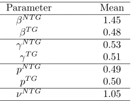
Table 3: Model averaged posterior summaries from the models fitted to the experimental data.
Parameter Number of parameters Posterior probability
β 1 0.21
2 0.79
γ 1 0.72
2 0.28
ν 0 0.7
1 0.3
p 1 0.58
2 0.42
Table 4: Model averaged posterior weights for the number of parameters of each type, from the models fitted to the experimental transmission data. Bold font highlights the specification with highest posterior support.
6
Application to experimental transmission study of AIV
We now apply our approach to the experimental transmission data from Lyall et al. (2011), shown in Figure1 and Table1. These data are openly available from the Uni-versity of Exeter’s institutional repository at:https://doi.org/10.24378/exe.1644. (Note that the measurements are now at half-day intervals, rather then daily intervals as per the simulation study.)
We used the same approach as in the Section5, using an initial tolerance ofini= 5 and a target tolerance of target = 2 in the first wave, and a fixed tolerance of ini =
target= 1 in the second wave. The target regions defined bytarget= 2 and 1 are shown in Supplementary Figure S11.
[image:26.612.170.440.256.365.2]