The cataclysmic variable QZ Lib : a period bouncer

warwick.ac.uk/lib-publications

Manuscript version: Author’s Accepted Manuscript

The version presented in WRAP is the author’s accepted manuscript and may differ from the

published version or Version of Record.

Persistent WRAP URL:

http://wrap.warwick.ac.uk/108942

How to cite:

Please refer to published version for the most recent bibliographic citation information.

If a published version is known of, the repository item page linked to above, will contain

details on accessing it.

Copyright and reuse:

The Warwick Research Archive Portal (WRAP) makes this work by researchers of the

University of Warwick available open access under the following conditions.

Copyright © and all moral rights to the version of the paper presented here belong to the

individual author(s) and/or other copyright owners. To the extent reasonable and

practicable the material made available in WRAP has been checked for eligibility before

being made available.

Copies of full items can be used for personal research or study, educational, or not-for-profit

purposes without prior permission or charge. Provided that the authors, title and full

bibliographic details are credited, a hyperlink and/or URL is given for the original metadata

page and the content is not changed in any way.

Publisher’s statement:

Please refer to the repository item page, publisher’s statement section, for further

information.

The cataclysmic variable QZ Lib: a period bouncer

A. F. Pala

1

?

, L. Schmidtobreick

2

†

, C. Tappert

3

, B. T. G¨

ansicke

1

and A. Mehner

2

1_{Department of Physics, University of Warwick, Coventry, CV4 7AL, UK} 2_{European Southern Observatory, Casilla 19001, Santiago 19, Chile}

3_{Institute of Physics and Astronomy, Universidad de Valpara´ıso, Av. Gran Bretana 1111, Valparaiso, Chile}

Accepted 2018 September 03. Received 2018 September 03; in original form 2018 January 17.

ABSTRACT

While highly evolved cataclysmic variables (CVs) with brown dwarf donors, often called “period bouncers”, are predicted to make up '40−70% of the Galactic CV population, only a handful of such systems are currently known. The identification and characterization of additional period bouncers is therefore important to probe this poorly understood phase of CV evolution. We investigate the evolution of the CV QZ Lib following its 2004 super–outburst using multi–epoch spectroscopy. From time– resolved spectroscopic observations we measure the orbital period of the system,Porb=

0.06436(20)d, which, combined with the superhump period PSH = 0.064602(24)d, yields the system mass ratio, q =0.040(9). From the analysis of the spectral energy distribution we determine the structure of the accretion disc and the white dwarf effective temperature, Teff = 10 500±1500 K. We also derive an upper limit on the effective temperature of the secondary,Teff .1700 K, corresponding to a brown dwarf of T spectral type. The low temperature of the white dwarf, the small mass ratio and the fact that the donor is not dominating the near–infrared emission are all clues of a post bounce system. Although it is possible that QZ Lib could have formed as a white dwarf plus a brown dwarf binary, binary population synthesis studies clearly suggest this scenario to be less likely than a period bouncer detection and we conclude that QZ Lib is a CV that has already evolved through the period minimum.

Key words: stars: dwarf novae, binaries: close, brown dwarfs – stars: individual: QZ Lib

1 INTRODUCTION

Cataclysmic variables (CVs) are close interacting binaries composed by a white dwarf (the primary) and a low–mass star (the donor or secondary). The secondary star fills its Roche–lobe and is therefore losing mass through the inner Lagrangian point. In the absence of strong magnetic fields, this matter is then accreted onto the white dwarf via an accretion disc (seeWarner 1995for a comprehensive review). For the mass transfer process to be stable, the system needs to lose angular momentum in order to continuously shrink and keep the secondary in touch with its Roche– lobe. Therefore, during their life, CVs evolve from long to short orbital periods (Porb) while angular momentum is

re-moved from the system by two mechanisms: magnetic brak-ing and gravitational wave radiation (Rappaport et al. 1983;

Paczynski & Sienkiewicz 1983;Spruit & Ritter 1983). The evolution proceeds towards shorter periods until the sys-tem reaches the “period minimum”, which theory predicts

? _{[email protected]} † [email protected]

to be Porb ' 70 min (Goliasch & Nelson 2015; Kalomeni

et al. 2016). At this stage the timescale at which the sec-ondary star loses mass becomes much shorter than its ther-mal timescale and thus the secondary stops shrinking in re-sponse to the mass loss. Consequently, systems that have passed the period minimum evolve back towards longer or-bital periods and, for this reason, are called “period bounc-ers”.

Although this standard model of CV evolution is widely accepted, a number of discrepancies between theory and ob-servations suggest that our current understanding of CV evolution remains incomplete. One of the major disagree-ments is found near the period minimum. The time that a CV spends at a given orbital period (and thus its detection probability at thatP_orb) is inversely proportional to the rate at whichPorbvaries. The evolution of CVs approaching the

2005,2006, 2007, 2009,2011), G¨ansicke et al.(2009) con-firmed the existence of this predicted pile–up of CVs at the period minimum. However, they also demonstrate that the observed period minimum ('83 min) is actually longer than the theoretically predicted ('70 min). Second,'40%( Go-liasch & Nelson 2015) to '70%(Kolb 1993;Knigge et al. 2011) of the present Galactic CV population is expected to have evolved past the period minimum. However, despite there are now more than 1400 CVs with an orbital period determination (Ritter & Kolb 2003), only a handful of period bouncercandidates have been so far identified (e.g. Patter-son et al. 2005b;Unda-Sanzana et al. 2008;Littlefair et al. 2006; Patterson 2011; Kato et al. 2015, 2016; McAllister et al. 2017; Neustroev et al. 2017). Therefore the identifi-cation of additional period bouncers and the determination of their physical parameters is important for a direct com-parison between the current models of CV evolution and observations in a region of the parameter space where very few objects are known.

One of the best parameters to identify a period bouncer is the mass ratio q=Msec/MWD. During the system

evolu-tion, donor stars in CVs continuously lose mass and, since the mass distribution of CV white dwarf is comparatively narrow and centred at'0.8 M(Zorotovic et al. 2011), the

mass ratio reflects the evolutionary stage of the system ( Pat-terson et al. 2005b;Knigge et al. 2011). In particular, for sys-tems with Porb'90 minthat have not yet evolved through

the period minimum (pre–bounce CVs), the expected mass ratio is q'0.13 while period bouncers at the same orbital period are expected to haveq'0.03 (Knigge 2006). Given the bifurcation of the CV evolutionary track at the period minimum, this difference further increases for longer period CVs (see for example figure 6 from Howell et al. 2001). Therefore the mass ratio is a discriminant between pre and post–bounce systems and provides a powerful tool to suc-cessfully identify period bouncer candidates when a direct spectroscopic detection of the secondary is not possible ( Pat-terson 2011;Kato et al. 2015,2016).

A measurement of the mass ratio can be obtained from superhumps, i.e. low–amplitude modulations observed in the light curve of short–period CVs during superoutbursts. These are sudden increases in the system brightness origi-nating from the combination of a thermal instability in the disc and the tidal interaction of its outer edge with the secondary (Osaki 1996). Below a critical mass ratio value (q'0.3,Whitehurst 1988), owing to the strong secondary tidal torque, the disc becomes elliptical and starts precess-ing, giving rise to the superhumps. Superhumps have peri-ods (PSH) typically a few percent longer than the orbital one.

Patterson et al.(2005a) andKato & Osaki(2013) calibrated an empirical relationship that allows to measure the system mass ratio from this period excess.

In February 2004, Pojmanski (VSNET–alert 7982) de-tected the outburst of a new eruptive star in Libra, QZ Lib (aka ASAS 153616–0839.1). Light curves taken worldwide re-vealed that the object showed periodic variability with a probably increasing period (Kiyota 2004), which was in-terpreted as growing superhumps with a final period of

P_sh = 0.06501(3)d (Kato 2004). QZ Lib was then spectro-scopically confirmed of being a dwarf nova into outburst by

Schmidtobreick et al.(2004).

QZ Lib was included byPatterson (2011) in his list of

Figure 1.SMARTSV–band finding chart of QZ Lib (circle,RA= 15h₃₆m_16.s_{0, Dec. = −08°39}0₀₇s_{.6) and the nine reference stars} used for the differential photometry (squares). The field of view is40×30, north is up, east to the left.

period bouncer candidates (see his table 3 and table 5) owing to its estimated low mass ratio (q=0.035±0.020,Patterson et al. 2005b). However, Patterson et al. (2005b) obtained this measurement from unpublished CBA (Center for Back-yard Astrophysics) data which where characterised by low signal–to–noise ratio (SNR). Here, we present new phase– resolved photometric and spectroscopic observations of this system, from which we derive a more reliable mass ratio that, combined with the spectral energy distribution analy-sis, demonstrates the period bouncer nature of the system.

2 OBSERVATION AND DATA REDUCTION

2.1 Spectroscopic observations

Spectroscopic observations of QZ Lib were obtained at sev-eral epochs in 2004 using EFOSC2 (ESO Faint Object Spec-trograph and Camera 2) at the 3.6–meter telescope on La Silla Observatory, Chile.

A set of three low resolution spectra, covering the wave-length range3860−8070˚A, were acquired on three different nights, one (2004 Mar 15), two (2004 May 1) and six (2004 Aug 27) months after the superoutburst, using grism # 6. Additional medium resolution spectra, covering the wave-length range 6280−8200˚A, were obtained in March 2004 and August 2004 using grism #10. These observations con-sisted of a series a consecutive spectra with exposure times varying between 300 s and 400 s.

The standard reduction of the data was performed us-ing IRAF1 (Tody 1986,1993). The bias level has been sub-tracted and the data have been divided by a flat field, which was normalised by fitting Chebyshev functions of high order

1 _{IRAF is distributed by the National Optical Astronomy}

Table 1.Summary of the observational details. The last column reports the time range spun by the individual dataset for a comparison with the orbital period of QZ Lib, 1.54 h.

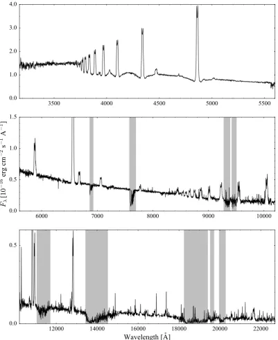
Date (UT) Tel./Inst. Grism/Slit/Filter R=λ/∆λ NExp tExp[s] ∆t[h]

2004-03-15 3.6/EFOSC2 Gr #6, 1.0” 323 3 600 0.53

2004-03-16 3.6/EFOSC2 Gr#10, 1.0” 915 30 400 3.62

2004-03-17 3.6/EFOSC2 Gr#10, 1.0” 915 15 300 1.40

2004-05-01 3.6/EFOSC2 Gr#6, 1.0” 323 3 600 0.53

2004-08-27 3.6/EFOSC2 Gr#6, 1.0” 323 3 900 0.78

2004-08-28 3.6/EFOSC2 Gr#10, 1.0” 915 6 400 0.72

2004-08-29 3.6/EFOSC2 Gr#10, 1.0” 915 26 400 3.14

2004-08-30 3.6/EFOSC2 Gr#10, 1.0” 915 11 400 1.33

2005-02-07 1.0–m SMARTS V 12 300 1.08

2005-02-09 1.0–m SMARTS V 19 300 1.71

2005-02-10 1.0–m SMARTS V 21 300 1.90

2005-02-11 1.0–m SMARTS V 17 300 1.53

2005-02-12 1.0–m SMARTS V 20 300 1.80

2005-02-13 1.0–m SMARTS V 22 300 1.99

2005-02-13 3.6/EFOSC2 V 145 20 2.13

2012-08-13 VLT/X–shooter UVB,VIS,NIR 1.0”, 0.9”, 0.9” 5400, 8900, 5600 6,6,7 244,252,249 0.50 2012-08-15 VLT/X–shooter UVB,VIS,NIR 1.0”, 0.9”, 0.9” 5400, 8900, 5600 4,4,4 244,252,249 0.33 2013-04-21 VLT/X–shooter UVB,VIS,NIR 1.0”, 0.9”, 0.9” 5400, 8900, 5600 24,24,24 244,252,249 1.98 2015-05-12 VLT/X–shooter UVB,VIS,NIR 1.0”, 0.9”, 0.9” 5400, 8900, 5600 9,7,7 410,465,510 1.11

Notes.∆t includes the overhead times:'34s for EFOSC2 imaging and spectroscopy,'25s for SMARTS imaging and '45s for X–shooter spectroscopy.

to remove the detector specific spectral response. All spec-tra have been optimally exspec-tracted following the method of

Horne (1986) and the low resolution spectra of each night have been averaged. Wavelength calibration yielded a final FWHM (full width at half–maximum) resolution of 12.8 ˚A for the low resolution data (grism # 6) and 5.5 ˚A for the medium resolution data (grism #10). All further analysis has been done using the ESO–MIDAS toolkit.

For the low resolution data, the instrument response function was corrected using spectroscopic standards. Since the nights have been clear but not photometric, we per-formed differential photometry on the acquisition files to de-termine the relative flux values of our object with respect to four comparison stars. The spectra were scaled accordingly. Hence, while the absolute zero–point is more uncertain, the relative flux calibration of the individual spectra and the flux differences between the three average spectra have an accuracy of about 4%.

High spectral resolution time–series spectroscopy was obtained with X–shooter at four epochs in 2012, 2013, and 2015. X–shooter is a medium–resolution ´echelle spectro-graph available at the Very Large Telescope (VLT) in Cerro Paranal (Chile,Vernet et al. 2011) since 2009. The instru-ment has been designed to cover in one exposure the wave-length range from ' 3 000˚A up to ' 25 000˚A. In order to do so, X–shooter is equipped with three arms: blue (UVB, λ ' 3000−5595˚A), visual (VIS, λ ' 5595−10 240˚A) and near–infrared (NIR,λ'10 240−24 800˚A). Spectra were ob-tained with slit widths of 1.000 in the UVB arm, 0.900 in the VIS arm, and 0.900 in the NIR arm and a 1×2 bin-ning yielding spectral resolving powers of R ∼ 5000−9000. The data processing was performed with the ESO Reflex X–shooter pipeline (version 2.4.0), which includes the stan-dard reduction steps of bias and dark current removal, order identification and tracing, flat-fielding, dispersion solution,

correction for instrument response and atmospheric extinc-tion, and merging of all orders.

QZ Lib is located at a galactic latitude of36.4◦ and at a distance of d=187±12pc, as determined from the Gaia parallax ($=5.3±0.3mas,Gaia Collaboration et al. 2016,

2018). This implies an interstellar extinction of E(B−V) =

0.09, based on the three–dimensional map of interstellar dust reddening based on Pan–STARRS 1 and 2MASS photome-try (Green et al. 2018). Such a small amount of interstellar extinction is negligible for the analysis presented here, and we hence show the spectra as observed, i.e. without redden-ing correction.

2.2 Photometric observations

Ma

r '04

Apr '

04

_Ma

y '04 Jun '

04

Jul '

04

Aug '

04

Sep '

04

10

12

14

16

18

20

22

Vi

sua

l m

agni

tude

(

V

)

Jan '

12

Jan '

13

Jan '

14

Jan '

15

Jan '

16

AAVSO

CRTS

ASAS

Figure 2. Light curve of QZ Lib from its first detection (superoutburst in February 2004) up to 2016. The grey arrows highlight the epochs of the EFOSC2 observations one month (grism # 6 and # 10), two months (grisms # 6) and six months (grisms # 6 and # 10) after the superoutburst. The black arrows highlight the three epochs in which X–shooter spectroscopy has been acquired.

0

2

4

6

8

10

12

14

16

JD [+2 456 400 days]

14

15

16

17

18

19

20

21

Vi

sua

l m

agni

tude

(

V

)

6.80

6.85

6.90

6.95

18.5

19.0

19.5

20.0

20.5

Figure 3. Ligthcurve of QZ Lib in a period of particular intense monitoring (17 April 2013 – 5 May 2013). The inset shows a sample close–up of the night of 24–04–2013: the system variability is dominated by flickering and no periodic variation is detected.

3 THE LIGHT CURVE

During the SMARTS and EFOSC2 observations, the bright-ness of QZ Lib is clearly varying, however, this variation is more of an irregular nature, with flickering and long–time variation dominating the light curves. We searched for peri-odic modulation using various Fourier techniques but did not find any persistent signal. Similar results can be derived from the photometric observations in the AAVSO (American As-sociation of Variable Star Observers) and CRTS (Catalina Real-time Transient Survey, Drake et al. 2009) databases (Figure 2): no orbital variation is detected even for those nights that are covered with ample data points (Figure3).

4 TIME RESOLVED SPECTROSCOPY

4.1 The orbital period

Time–resolved spectroscopic observations of QZ Lib were ob-tained with the EFOSC2 medium resolution grism # 10 on

2004 March 16-17 and 2004 August 28-30. Each set of ob-servation covered about 1.5 orbits. The system had retuned to the quiescent state by the time of the August observa-tions, as can be inferred from the additional low resolution EFOSC2 spectroscopic observations described in Section5. The average spectrum obtained during the August EFOSC2 grism # 10 observations is shown in Figure4. The Hα emission line shows a double-peaked morphology, aris-ing from the Keplerian velocity distribution of the gas in the disc (Marsh & Horne 1988). Since the disc is centred on the white dwarf, the Doppler shift of the Hαline traces the mo-tion around the centre of mass of the system and provides a measurement of the orbital period. We therefore measured the radial velocity of the Hαemission line by fitting a sin-gle broad Gaussian to it. A more complex fitting procedure, e.g. using multiple Gaussians (Shafter 1983), may provide a better fit to the double-peaked structure, but will not result in a more accurate determination of the orbital period.

6500

6550

6600

6650

Wavelength [

]

0.0

0.2

0.4

0.6

0.8

1.0

Norm

ali

sed fl

ux

Figure 4.EFOSC2 average spectrum of QZ Lib around theHα

emission line, obtained with the grism # 10 six months after its 2004 superoutburst. As shown by the additional spectroscopic observations presented in Section5, the system had returned to the quiescent level at the time of these observations.

Figure 5.Scargle periodograms for the March (top) and August (middle) EFOSC2 datasets. The power is shown on the y-axis, where an arbitrary scale is used for illustration purposes. The EFOSC2 datasets shows one strong peak in common, which we assumed to belong to the orbital period (vertical solid line and dashed lines for the related uncertainties). The same peak is also identified in the periodogram computed using all the EFOSC2 and the X–shooter observations (bottom). These observations are more than ten years apart and therefore the inclusion of the X– shooter data does not allow to improve the precision of the orbital period.

of both data sets show several alias peaks but only one fre-quency yields a strong signal in both, which we concluded to belong to the orbital period (see Figure 5). Since the August dataset has higher SNR and is slightly longer than the March dataset, we used it to determine the orbital pe-riod, which results inPorb=0.06436(20)d or1.545±0.005h,

in good agreement with the measurement by Thorstensen et al.(2017), Porb=0.06413(8)d. Unfortunately, the March

and August sets are too far apart in time to allow the

com-0.0 0.5 1.0 1.5 2.0

Orbital phase [

,

]

−50 0 50

Ra

dia

l V

eloc

ity [km

/s]

Figure 6.The EFOSC2 August data are plotted in phase using the orbital periodPorb=0.06436(20)d; the zero-phase corresponds toHJD=2 453 246.5050. Two phases are plotted for clarity, the first one has the uncertainties of the individual measurements overplotted. The grey line gives the best sinusoidal fit to the data.

bination of the data to increase the accuracy. In addition, some time–series spectroscopy at higher spectral resolution was taken with X–shooter during three epochs in 2012, 2013 and 2015 which we used to verify the orbital period. How-ever, the longest X–shooter dataset from April 2013 covers less than two orbits and therefore does not allow to improve the precision of the orbital period. Moreover, the X–shooter and EFOSC2 data sets are too far apart in time to be com-bined and improve the uncertainty of the period determina-tion.

In a circular orbit, the radial velocity, V, of the Hα

emission line varies in a sinusoidal way during one orbital cycle:

V =γ+KEsin(2πφ) (1)

where γ is the systemic velocity of the system, KE is the

radial velocity amplitude of the emission lines andφ is the orbital phase of the spectrum. Given the higher quality of the August EFOSC2 dataset, we used these time–resolved observations to computeγand KE. From a sinusoidal least

squares fit to the data, we foundγ=−1.6±1.5km s−1 and

KE = 37±2km s−1. The uncertainties on these quantities

were determined by computing Monte–Carlo simulations of the fit. The best fit returns the following ephemeris for the red to blue crossing of the emission lines:

HJD=2 453 246.5050(6)+0.06436(20) E (2) We then used this ephemeris to calculate the orbital phase for all data points of the August 2004 data set (Figure6).

4.2 Doppler Tomography

Doppler tomography makes use of the orbital variation of the emission line profiles. Each point of the emission line can be attributed to a radial velocity, which can be transformed to (vx,vy)for a given phase. The Doppler mapsI(vx,vy)display the flux emitted by gas moving with the velocity(vx,vy)and thus show the emission distribution in velocity coordinates with the centre of mass at (0,0). We used the code ofSpruit

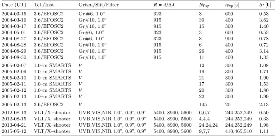
Figure 7.Diagnostic diagram for the Hαemission line, showing the parameters of the radial velocity fit as function of the Gaus-sian separation. For separations between 17˚A and 28˚A, where σ(K1)is minimal, the outer wings of the lines are sampled.

routines (Tappert et al. 2003) and the largest contiguous data set with the highest spectral resolution – the X–shooter data from April 2013 – for these computations.

The spectral resolution of the X–shooter data (R '

7000) allows to accurately trace the motion of different parts of the disc which can be used to calculate the diagnostic di-agram of the system (Shafter 1983) and better constrain the Doppler maps. This method allows to measure the orbital velocity of the white dwarf (KWD) by probing the wing of

the emission lines. This because the wings arise from the inner region of the accretion disc and therefore trace more accurately the motion of the white dwarf than the core of the emission line, which instead originates in the outer disc. In the case of the line emission originating exclusively in a perfectly circular disc, the full emission line profile would re-flect the motion of the white dwarf, i.e.KE=KWD. Instead,

the symmetry of the outer disc is usually perturbed by the impact of the accretion stream, and additional emission com-ponents from this region and/or the potentially irradiated secondary star often contribute to the centre of the emission line, so that different parts of the emission line may corre-spond to different radial velocity amplitudes and phases (e.g.

Horne & Marsh 1986). In consequence, for measurements of the full line profile, usuallyKE,KWD.

We therefore measuredKWDin an iterative way,

adopt-ing the orbital period as determined from the analysis of the EFOSC2 data (see Section 4.1) and using two Gaus-sians of 4 ˚A of FWHM to fit the Hα emission lines in the phase resolved X–shooter observations from April 2013. The separation of the two Gaussians was varied between 1 ˚A and

500

0

500

vel_x [km/s]

500

0

500

vel_y [km/s]

H

500 0

500

v_rad [km/s]

0.0

0.5

1.0

1.5

orbital phase

500

0

500

vel_x [km/s]

500

0

500

vel_y [km/s]

H

500 0

500

v_rad [km/s]

0.0

0.5

1.0

1.5

orbital phase

Figure 8.The Doppler maps show the emission line distribution in velocity coordinates for Hα(upper plot) and Hβ(lower plot). In the panel on the right, the trailed spectra of the respective emission line are plotted in velocity coordinates. Two phase cycles are plotted for clarity.

42 ˚A to gradually exclude the core of the line. For each sepa-ration, a radial velocity curve was produced and fitted with a sinusoidal function as defined in Equation1. The resulting velocity amplitudes K1 as a function of the separations of

the two Gaussians are shown in Figure7. Once the separa-tion of the Gaussians is sufficient to exclude the perturbed core of the emission line, the velocity amplitude and the or-bital phase remain roughly constant, and the most robust measurements of these two parameters is taken from the range of separations whereσ(K1) is minimal. In this case,

this corresponds to separations between 17 ˚A and 28 ˚A, con-sistent with those values where the uncertainty σ(K₁) has a minimum. To determine the zero-phase as input for the Doppler tomography, as well as the radial velocity ampli-tude of the white dwarf, we calculated the average values for this range of separations. For the white dwarf, we thus derivedKWD=20±4 km s−1.

as emission from the bright spot, the point where the accre-tion stream hits the disc. The emission from the bright spot is also visible as a thin S–curve with a velocity amplitude consistent with the outer disc velocity in the trailed spectra shown in the right–hand side panels.

The presence of this isolated emission source explains the variation ofK₁within the diagnostic diagram as well as the difference between KE =37 kms−1 as determined from fitting a broad Gaussian andKWD=20 kms−1as determined

from the diagnostic diagram. The fit of a single broad Gaus-sian to the complicated structure of the emission line is influ-enced by the isolated emission source and does not represent the motion of the white dwarf.

4.3 The mass ratio

From the orbital period Porb = 0.06436(20)d and the

re-ported superhump periodPSH=0.064602(24)d (Kato 2015),

we derived a period excess of=(PSH−Porb)/Porb=0.0038.

Using the empirical formula = 0.18q+0.29q2 (Patterson et al. 2005a), we find the mass ratioq=0.020±0.017. This value is consistent with the previously determined one by

Patterson et al.(2005b,q=0.035±0.020). We consider our measurement a more reliable result since their orbital period was tentatively derived from photometric variations (Patter-son, private communication) which we consider problematic due to strong non–periodic contributions like flickering and long-term variations.

Since PSH varies with time, the −q relationship can

be applied at different stages (i.e. using different superhump periods) of the superoutburst.Kato et al. (2009) identified three superhump stages: (A) an early phase where PSH has

the highest value; (B) an intermediate phase with a sta-bilised PSH and (C) a final phase with a shorter PSH. In

the traditional way of determiningqfrom the period excess (Patterson et al. 2005a; Kato et al. 2009;Patterson 2011),

PSHdetermined during stage B is commonly used. However,

Kato & Osaki(2013) argue that thisPSHsystematically

un-derestimates q for low mass–ratio systems (q . 0.09) and they present an alternative−qrelationship calibration from stage A superhumps. The mass–ratio we derived for QZ Lib lies in the range affected by this systematic effect and there-fore we re–computed the value of q using equation 5 from

Kato & Osaki(2013), using the stage A superhump period of QZ Lib fromKato et al.(2015,PSH=0.06557(14)d), finding q=0.048±0.010.

The mass ratios derived with the two−qcalibrations, respectively q =0.020±0.017 (obtained using the method byPatterson et al. 2005a) andq =0.048±0.010(obtained using the method byKato & Osaki 2013) agree within the uncertainties (on a'1.4σ level). Assuming one instead of the other does not affect the conclusions drawn in the fol-lowing Sections, in which we assume the weighted average of the two:q=0.040±0.009.

5 THE SPECTRA

5.1 The model

In the optical spectrum of a CV, three main light sources contributes to the emission of the system: the white dwarf,

4000 4500 5000 5500 6000 6500 7000 7500

Wavelength [

]

0.0

0.5

1.0

1.5

2.0

Fλ

[

10

−

15

erg c

m

−

2

s

−

1Å

−

1

]

2004

03

15

2004

05

01

2004

08

27

Figure 9. EFOSC2 spectrophotometric calibrated spectra of QZ Lib obtained one (black), two (dark grey) and six (light grey) months after its 2004 superoutburst. The regions contaminated by telluric absorption bands are highlighted in grey.

Table 2. Range of variations for the free parameters in the slab model describing the emission from accretion disc.

Parameter Value

Effective temperature (K) 5700−8000

Pressure (dyn cm−2) 0−1000

Radial velocity (km s−1) 0−2000

Inclination (°) 0−60

Geometrical height (cm) 0−1010

Notes.The upper limit on the inclination is set by the fact that no eclipse is detected in the light curve of QZ Lib.

the secondary star and the accretion disc. The white dwarf, which is heated by the energy released by the compres-sion of the accreted material (Sion 1995;Townsley & Bild-sten 2003), is usually hot with an effective temperature

T_eff &10 000K (Sion 1999), and thus dominates in the blue part of the spectrum. The donor is typically a cold low– mass star which starts contributing in the near–infrared (λ & 7000˚A). Finally, strong emission lines, whose shape and width are determined by the Keplerian velocity distri-bution of the accreting material, reveal the presence of the disc.

From a spectral fit to a CV spectrum with synthetic models accounting for the contribution from these three sources, it is possible to determine the effective temperatures of the white dwarf and the secondary star. We usedtlusty andsynspec(Hubeny 1988;Hubeny & Lanz 1995) to com-pute a grid of white dwarf atmosphere models covering the rangeTeff =9000−40 000K in steps of 100K and assuming

a metallicity ofZ =0.01Z, (as determined from the

Table 3. Cooling sequence for the white dwarf in QZ Lib after its 2004 super–outburst.

Date Teff(K)

2004–03–15 17 000±2000

2004–05–01 14 000±600

2004–08–27 11 700±250

correlates with its surface gravity: strong gravitational fields translate into pressure broadening of the lines; this effect can be balanced by higher temperatures that increase the frac-tion of ionised hydrogen, resulting in narrower absorpfrac-tion lines. Moreover, in CVs, the Balmer line cores, commonly used to simultaneously constrain the effective temperature and the surface gravity of isolated white dwarfs (see for ex-ample Gianninas et al. 2011), are often contaminated by strong disc emission lines. For these reasons, it is not possible to constrain bothTeff andloggof the white dwarf in QZ Lib

from the analysis of optical data and we therefore generated our grid of models assuming logg =8.35, corresponding to the average mass of CV white dwarfs (MWD=0.83±0.23 M,

Zorotovic et al. 2011). Assuming the mass–radius relation-ship fromHamada & Salpeter(1961), this value oflogg cor-respond to a white dwarf radius of RWD =0.01 R (the

as-sumption of the zero-temperature mass–radius relationship is sufficient given the low temperature of the white dwarf).

As discussed byPala et al.(2017), the correlation be-tween the white dwarf logg and T_eff introduces a system-atic uncertainty in the effective temperature measurement (see figure 8 from Pala et al. 2017) which is of the order of '200K forTeff '11 000K and increases up to'1000K

forTeff '17 000K. In order to account for its effect, in the

following, we assumed as uncertainty on our effective tem-perature determinations the largest between (i) the statis-tical uncertainty returned by our fitting procedure and (ii) the corresponding systematic uncertainty related to the un-known mass of the white dwarf (as determined from equa-tion 2 from Pala et al. 2017). In this way, our analysis ac-counts also for the uncertainty of the mass distribution of CV white dwarfs.

To approximate the disc emission, we used an isother-mal and isobaric pure–hydrogen slab model, as described inG¨ansicke et al.(1997,1999). The free parameters of this model and their allowed ranges are reported in Table2.

Finally, the last contribution that needs to be taken into account is the emission from the donor star. From the knowledge of the system mass ratio and from our previous assumption ofMWD=0.8 M, we determined the mass of the

secondary star, Msec=0.032±0.012 M. The orbital period

of the system and Kepler’s third law return a measurement of the orbital separation, a=0.63±0.05 R. Since the

sec-ondary is filling its Roche–lobe, its radius is defined by the relationship (Eggleton 1983):

Rsec=

a0.49q2/3

0.6q2/3+ln(1+q1/3) (3) and results in Rsec = 0.10 ± 0.01 R. The combination

Msec and Rsec returns the surface gravity of the donor,

log(g[cm s−2])=4.9±0.2. The typical effective temperature of donor stars in short–period CVs are 500 K.Teff . 3000 K

(Knigge 2006). The metallicity of the white dwarf

repre-4000

4500

5000

5500

6000

Wavelength [

Å

]

0.0

0.2

0.4

0.6

0.8

1.0

1.2

F

[

10

−

15

erg c

m

−

2

s

−

1

Å

−

1

]

H

β

H

γ

H

δ

H

ǫ

He

I

He

I

2004

−

08

−

27

T =

11 700 ± 250

K

Figure 10.EFOSC2 spectrum of QZ Lib (light grey) taken on 2004–08–27. The #6 grism is affected by a second–order contam-ination which reduces the useful wavelength range to6200˚A. At these wavelengths the possible contribution of the donor is negli-gible and thus we fitted the data including the contribution of a white dwarf (dotted line) and an isothermal and isobaric pure hy-drogen slab (dashed line) to approximate the disc emission. The sum is given by the black solid line.

sents a lower limit on the metallicity of the accreted mate-rial, which is stripped from the secondary photosphere. We therefore assumed that the secondary has the same metal-licity as the white dwarf, Z=0.01Z. However, at present,

none of the available model grids for late–type stars for

Z = 0.01Z cover the required range in temperature. We

therefore retrieved a grid of BT–Dusty (Allard et al. 2012) models for late–type stars from the Theoretical Spectra Web Server2, extending from Teff = 1000K (T6 spectral type)

up toTeff = 3600K (M2 spectral type), for logg = 5 and Z=0.3Z, which is the widest grid of available models with

the lowest metallicity value.

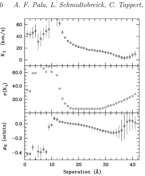
Fixing the distance to the system tod=187pc, as de-rived from the Gaia parallax, we then used a χ2 minimi-sation routine to fit our grid of models to the optical spec-tra. In the fitting procedure, we did not include the wave-length ranges of the telluric absorption features arising in the Earth’s atmosphere and, to better constrain the contri-bution of the disc to the overall emission, we allowed as free parameters the areas of the emission lines Hβ, Hγ, Hδand H. In the case of the X–shooter spectra we included also the areas of the emission lines Hα, Paδand Paζ.

We present the results of the fit to the different datasets in the following Sections.

2

Wavelength [

Å

]

F

[

10

−

16

erg c

m

−

2

s

−

1

Å

−

1

]

3500

4000

4500

5000

5500

0.0

1.0

2.0

3.0

4.0

6000

7000

8000

9000

10000

0.0

0.5

1.0

1.5

12000

14000

16000

18000

20000

22000

0.0

0.5

Figure 11.Averaged X–shooter spectrum of QZ Lib (UVB, top panel; VIS middle panel; NIR, bottom panel). The white dwarf signature is recognisable in the broad Balmer lines in the UVB arm. Strong emission lines arise from the accretion disc. No features from the secondary are detected in the near–infrared, which is contaminated by broad telluric absorption bands (highlighted in grey) and residuals from the sky line removal.

5.2 The spectra during the cooling towards

quiescence

The spectrophotometric calibrated low resolution EFOSC2 spectra of three epochs are plotted in Figure 9. The white dwarf is dominating the continuum in all of them, as seen from the clear presence of its broad Balmer absorption lines. The spectrum taken on 2004–03–15 still has a noticeable contribution of the accretion disc which then decreases at the later epochs.

Unfortunately, we noticed after the observations that

the grism # 6 of EFOSC2 is affected by a second–order con-tamination starting around 6000 ˚A. Hence, no conclusions can be made for the cool donor star and only the blue part of the spectrum was used for the fit of the white dwarf and the accretion disc.

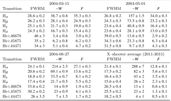
effec-Table 4.The evolution of FWHM (in ˚A), equivalent widthW(in ˚A), and line fluxF(in10−15_{erg cm}−2_s−1_{) for the main Balmer and He} i emission lines in the spectra of QZ Lib. Note that the uncertainty of the line flux accounts for the uncertainty of the relative flux in the line but does not include the errors introduced in our spectrophotometric flux calibration procedure (see Section2.1).

2004-03-15 2004-05-01

Transition FWHM −W F FWHM −W F

Hα 28.6±0.2 38.7±0.8 35.3±0.3 26.8±0.2 157±1.5 34.0±0.3

Hβ 26.2±0.3 28.1±0.4 24.9±0.3 24.3±0.3 73.5±0.8 23.2±0.3

Hγ 25.1±0.3 21.7±0.3 19.0±0.3 23.6±0.4 40.8±0.9 16.4±0.3

Hδ 24.5±0.2 16.7±0.3 15.4±0.2 23.6±0.4 28.1±0.9 13.0±0.5

Heiλ6678 46±3 3.4±0.6 3.0±0.2 39.0±0.5 13.6±0.5 2.9±0.2

Heiλ5875 35±2 6.2±0.8 6.2±0.3 34.3±0.6 23.3±0.8 6.3±0.4

Heiλ4471 34±3 5.1±0.4 4.7±0.2 31.5±0.8 9.7±0.5 4.3±0.3 2004-08-27 X–shooter average (2011-2015)

Transition FWHM −W F FWHM −W F

Hα 24.1±0.1 214±2.5 27.1±0.3 21.4±0.1 288±7 12.8±0.1

Hβ 20.6±0.2 69.1±0.9 13.6±0.2 17.5±0.2 82±3 5.6±0.1

Hγ 18.8±0.3 33.5±0.7 8.1±0.2 16.4±0.5 43±2 3.5±0.1

Hδ 17.4±0.4 21.7±0.5 5.5±0.2 15.6±0.4 26±2 2.3±0.1

Heiλ6678 33.6±0.2 14±0.9 1.9±0.2 26.5±0.4 13±1 0.6±0.1

Heiλ5875 30.2±0.2 23±0.9 4.1±0.3 25.5±0.2 23±2 1.3±0.1 Heiλ4471 26±3.5 7±1.5 1.7±0.2 18.2±0.5 4±1 0.5±0.1

tive temperature of17 000±2000K. The strong continuum contribution arising from the disc and the contamination from the emission lines in the 2004–03–15 spectrum prevent a more accurate measurement of the white dwarf effective temperature.

For the 2004–08–27 we measured a white dwarf effec-tive temperature of'11 700K (Figure10). From the best fit model we found that the isothermal hydrogen slab is opti-cally thin with a temperature of about6200K. These values are consistent with the accretion disc model of quiescent dwarf novae (Williams 1980;Tylenda 1981).

5.3 The quiescence spectra

The X–shooter average spectrum of QZ Lib, taken about ten years after its super–outburst is shown in Figure 11. We compared the X–shooter spectra from the different years, i.e. 2012, 2013, and 2015 but found no difference and hence combined them to increase the SNR. This late spectrum differs from the spectra obtained within the first year of the outburst, showing stronger Balmer and helium emission lines, typical of a dwarf nova disc in quiescence (Table4).

We inspected the red part of the spectrum for ab-sorption features arising from the secondary photosphere. Typically, when the donor star dominates the near–infrared emission, the most prominent absorption lines are Na_i

11 381/11 403˚A, Ki 11 690/11 769˚A and 12 432/12 522˚A. However we could not identify any of those and therefore we assumed that the companion star contribution is negligible. We performed a spectral fit to the X–shooter data including a white dwarf and an hydrogen slab in the model. The best– fit model is shown in the top panel of Figure12and returns a white dwarf effective temperature ofTeff=10 500±1500 K,

in agreement with the value determined byPala et al.(2017,

Teff =11 303±238 K) from the analysis of ultraviolet data.

The best–fit parameters for the hydrogen slab are listed in Table 5 while the overall system parameters derived from

Table 5.Best fit parameters for the isothermal and isobaric hy-drogen slab describing the emission from accretion disc in QZ Lib.

Hydrogen slab parameter Value

Effective temperature (K) 7100±300

Pressure (dyn cm−2) 110±40

Radial velocity (km s−1) 1150±250

Inclination (°) 30±12

Geometrical height (cm) 1.2(2)×107

the analysis of the EFOSC2 and X–shooter data are listed in Table6.

Although a clear signature of the companion star can-not be identified in the X–shooter data, only accounting for the white dwarf and the slab emission does not allow to ad-equately reproduce the observed flux level forλ&10 000˚A. We therefore subtracted the white dwarf and the slab model to the X–shooter data and fit the grid of low–mass main sequence star (see Section 5.1) to the residual spectrum, constraining the secondary to be at the same distance as the white dwarf. The best–fit model is shown in the bottom panel of Figure12and returns a secondary star effective tem-perature ofT_eff '1700 K. A discussion on the interpretation of this infrared excess is presented in the next Section.

6 DISCUSSION

We used VLT/X–shooter optical and near–infrared spec-troscopy to reconstruct the Spectral Energy Distribution (SED) of QZ Lib, from λ ' 3000˚A out to λ ' 23 000˚A. From a spectral fit to the data, we have shown that the con-tribution from a white dwarf and an isothermal slab cannot adequately reproduce the flux in the red portion of the spec-trum. This infrared excess can be explained by either the accretion disc and/or a brown dwarf secondary star.

0.0 0.2 0.4 0.6 0.8 1.0 0.0

0.2 0.4 0.6 0.8 1.0

F

[erg c

m

−

2

s

−

1

Å

−

1

]

5000

10000

15000

10

10

10

10

⊕

⊕

⊕

X

−

shooter data

White dwarf

Hydrogen slab

Best

−

fit model

5000

10000

20000

Wavelength [

Å

]

10

10

10

10

10

⊕

⊕

⊕

X

−

shooter data

White dwarf

Hydrogen slab

Secondary

Best

−

fit model

Figure 12.X–shooter average spectrum of QZ Lib (grey) along with the best–fit model (red) which is composed of a white dwarf (blue) and an isothermal and isobaric hydrogen slab (cyan) and a brown dwarf companion (magenta, bottom). The Earth’s symbols highlight the position of the strongest telluric absorption bands, which were not included in the fit. A colour version of this figure is available in the electronic version of the manuscript.

in the fit procedure is a good model to account for the emis-sion lines that arise from the optically thin upper layers of the disc. However, if the central and colder regions of the disc are composed of an optically thick gas, they could contribute to the overall SED of the system in the form of an additional blackbody(–like) emission that is not accounted for by our model. At present, not much is known about the spectrum arising from the cool portion of quiescent discs. In the past, this contribution has been modelled by dividing the disc into several annuli and then summing the emission of each annu-lus, approximated as a blackbody with an effective tempera-ture set accordingly to the distance of the annulus from the white dwarf (Howell et al. 2006;Brinkworth et al. 2007; How-ell et al. 2008). Moreover, since this gas has a similar com-position and effective temperature as the secondary, is very

5000

10000

15000

20000

Wavelength [

Å

]

10−19

10−18

10−17

10−16

10−15

F

[erg c

m

−

2

s

−

1

Å

−

1

]

X

−

shooter data

M

−

dwarf companion, d = 187 pc

Figure 13.X–shooter spectrum of QZ Lib (black) in comparison with the expected emission of a M6.5–dwarf companion as typical for a pre–bounce system withPorb'90 minat a distanced=187pc (grey) as derived from theGaiaparallax.

80 85 90 95 100 105 110 115

P

_orb

[min]

0.05 0.10 0.15 0.20

q

80 85 90 95 100 105 110 115

P

_orb

[min]

1500 2000 2500 3000

T

sec

[K

]

0.060 0.065 0.070 0.075

P

_orb

[d]

0.060 0.065 0.070 0.075

P

_orb

[d]

Figure 14.QZ Lib mass ratio (left) and the upper limit on the effective temperature of its donor star (right) in comparison with the CV evolutionary track fromKnigge et al.(2011, solid line, calculated assuming MWD=0.8 Mfor the left panel). These measurements clearly suggests a period bouncer system rather than a pre–bounce CV.

Although we cannot distinguish between the emission of the donor star and that of a possibly optically thick cool accretion disc, given the mass ratio of QZ Lib, q =

0.040(9), we can still conclude that its donor star must be a brown dwarf. In fact, considering a white dwarf mass

0.6 M . MWD . 1.44 M, the secondary star mass

re-sults0.024 M.Msec.0.058 M, i.e. below the hydrogen–

burning limit and clearly in the brown dwarf regime. Fur-thermore the expected spectral type of the donor star in a

pre–bounce CV at P_orb'90 minis M6.5, corresponding to

Msec = 0.096 M,Rsec=0.144 R andTeff =2744 K(Knigge

2006), is not consistent with the observed SED. In fact, such a star would clearly dominate the spectral appearance for λ & 7000˚A (Figure13). Instead, our fit to the X–shooter data shows that the upper limit on the secondary effective temperature isTeff'1700 K, supporting the conclusion of a

brown dwarf donor star (Figure14, right panel).

Table 6.System binary parameters for QZ Lib.

System parameter Value Instrument/Reference

Porb(min) 92.7±0.3 EFOSC2

q 0.040±0.009 EFOSC2

d(pc) 187±12 Gaia

i(°) 30±12 X–shooter

Teff(K) 10 500±1500 X–shooter

Tsec(K) .1700 X–shooter

γ(km s−1_{) −1.6±1.5 EFOSC2}

KWD(km s−1) 20±4 X–shooter

logg 8.35 fixed

MWD(M) 0.8 fixed

RWD(R) 0.01 fixed

Msec(M) 0.032 fixed

Rsec(R) 0.10 fixed

the system mass ratio, is one of the strongest discriminants between pre and post–bounce systems (see e.g. figure 6 from

Howell et al. 2001). Inspecting the location of QZ Lib in the

Porb−q distribution shown in the left panel of Figure 14

strongly suggests that it is in the regime of potential period bouncers, rather than on the pre–bounce evolutionary track. Owing to its low mass ratio QZ Lib has been previously sug-gested as a potential period bouncer by Patterson (2011) and, subsequently, also byPala et al. (2017) because of its cool white dwarf. Our fit to the SED of QZ Lib provides ad-ditional support in favour of the period–bouncer nature of QZ Lib.

Alternatively, QZ Lib could have been born with a brown dwarf donor star. These kind of binaries start mass transfer below the period minimum and then evolve to-wards longer orbital periods, finally merging into the stan-dard track of period bouncers (figure 1 fromKolb & Baraffe 1999). Even if this scenario cannot be ruled out, the popu-lation synthesis study fromPolitano(2004) has shown that CVs hosting brown dwarf donors with orbital periods above the period minimum are four times more likely to have fol-lowed the standard path of CV evolution (i.e. the donor has become substellar as a consequence of mass erosion during the CV evolution) than being born as a white dwarf plus brown dwarf binary, suggesting that QZ Lib is more likely a period bouncer CV.

7 CONCLUSIONS

We present photometric and spectroscopic time–resolved ob-servations of the cataclysmic variable QZ Lib. From radial velocity measurements of the Hαemission line, we determine the orbital period Porb=0.06436(20)d that, combined with

the superhump period, PSH =0.06557(14)d, yields the

sys-tem mass ratio,q=0.040±0.009. Assuming the mass of the white dwarf to be in the range0.6 M . MWD . 1.44 M,

we found that the secondary mass is 0.024 M . Msec .

0.058 M, and therefore the donor must be a brown dwarf.

From a spectral fit to the averaged X–shooter spec-trum we measure the white dwarf effective temperature,

Teff=10 500±1500 K. Modelling the data with a white dwarf

and an isothermal and isobaric hydrogen slab does not ad-equately reproduce the observed flux in the reddest portion of the spectrum. Interpreting this weak infrared excess as

the contribution from the donor star implies an upper limit on its effective temperature, Tsec . 1700 K. However, this

excess could also originate from an optically thick accre-tion disc. The limited wavelength range of our observaaccre-tions does not allow to further investigate this possibility but, if the near–infrared excess arises from the disc, it would im-ply the presence of an even colder secondary star, bringing our results into an even better agreement with the predicted evolutionary track of the period bouncer CVs.

Although we cannot exclude that QZ Lib is born with a brown dwarf donor, this scenario would be four times less likely than the detection of a period bouncer CV. We there-fore argue that QZ Lib is a CV that has evolved through the period minimum. In fact, QZ Lib meets all the requirements for being a period bouncer: it has a brown dwarf companion, a low mass ratio and hosts the coolest white dwarf at the longest orbital period (see its position in figure 21 fromPala et al. 2017). This is the first CV for which all these require-ments have been spectroscopically confirmed, ruling out a pre–bounce system still on its way to the period minimum and, instead, making QZ Lib the strongest period bouncer candidate identified so far.

The detection of period bouncer CVs is an important test for the theoretical prediction of the standard model of CV evolution, accordingly to which'40−70%(Kolb 1993;

Knigge et al. 2011;Goliasch & Nelson 2015) of the present Galactic CV population is expected to have evolved past the period minimum. However, despite more than 40 years of in-tense research on CVs which has led to the identification of over 1400 systems with an orbital period determination ( Rit-ter & Kolb 2003), only a handful of period bouncer have so far been identified. QZ Lib illustrates how some of these elu-sive systems could be hiding among the known CVs but have not been identified as such owing to the limited wavelength range in which they have been studied so far. We illustrated how multi–wavelength observations, extending from the ul-traviolet to the infrared, are one of the most powerful tool to unveil this major component of the present day Galactic CV population.

ACKNOWLEDGEMENTS

Based on observations made with ESO Telescopes at La Silla and Paranal Observatories under programme ID 60.A-9013(A), 089.D-0421(A), 095.D-0802(A).

This work has made use of data from the European Space Agency (ESA) mission Gaia (https://www.cosmos.esa. int/gaia), processed by the Gaia Data Processing and Analysis Consortium (DPAC, https://www.cosmos.esa. int/web/gaia/dpac/consortium). Funding for the DPAC has been provided by national institutions, in particular the institutions participating in the Gaia Multilateral Agree-ment.

The research leading to these results has received funding from the European Research Council under the European Union’s Seventh Framework Programme (FP/2007–2013) / ERC Grant Agreement n. 320964 (WDTracer).

Val-para´ıso (CAV).

We acknowledge with thanks the variable star observations from the AAVSO International Database contributed by ob-servers worldwide and used in this research.

REFERENCES

Allard F., Homeier D., Freytag B., 2012, Philosophical Transac-tions of the Royal Society of London Series A, 370, 2765 Brinkworth C. S. et al., 2007, ApJ, 659, 1541

Drake A. J. et al., 2009, ApJ, 696, 870 Eggleton P. P., 1983, ApJ, 268, 368

Gaia Collaboration, Brown A. G. A., Vallenari A., Prusti T., de Bruijne J. H. J., Babusiaux C., Bailer-Jones C. A. L., 2018, ArXiv e-prints

Gaia Collaboration et al., 2016, A&A, 595, A1

G¨ansicke B. T., Beuermann K., Thomas H.-C., 1997, MNRAS, 289, 388

G¨ansicke B. T. et al., 2009, MNRAS, 397, 2170

G¨ansicke B. T., Sion E. M., Beuermann K., Fabian D., Cheng F. H., Krautter J., 1999, A&A, 347, 178

Gianninas A., Bergeron P., Ruiz M. T., 2011, ApJ, 743, 138 Goliasch J., Nelson L., 2015, ApJ, 809, 80

Green G. M. et al., 2018, ArXiv e-prints Hamada T., Salpeter E. E., 1961, ApJ, 134, 683 Horne K., 1986, PASP, 98, 609

Horne K., Marsh T. R., 1986, MNRAS, 218, 761 Howell S. B. et al., 2006, ApJ, 646, L65

Howell S. B., Hoard D. W., Brinkworth C., Kafka S., Walentosky M. J., Walter F. M., Rector T. A., 2008, ApJ, 685, 418 Howell S. B., Nelson L. A., Rappaport S., 2001, ApJ, 550, 897 Hubeny I., 1988, Computer Physics Communications, 52, 103 Hubeny I., Lanz T., 1995, ApJ, 439, 875

Kalomeni B., Nelson L., Rappaport S., Molnar M., Quintin J., Yakut K., 2016, ApJ, 833, 83

Kato T., 2004, vsnet-campaign-dn, 4126,7,8 Kato T., 2015, PASJ, 67, 108

Kato T. et al., 2015, PASJ, 67, 105 Kato T. et al., 2016, PASJ, 68, 65 Kato T. et al., 2009, PASJ, 61, S395 Kato T., Osaki Y., 2013, PASJ, 65, 115 Kiyota S., 2004, vsnet-campaign-dn, 4123,4 Knigge C., 2006, MNRAS, 373, 484

Knigge C., Baraffe I., Patterson J., 2011, ApJS, 194, 28 Kolb U., 1993, A&A, 271, 149

Kolb U., Baraffe I., 1999, MNRAS, 309, 1034

Littlefair S. P., Dhillon V. S., Marsh T. R., G¨ansicke B. T., South-worth J., Watson C. A., 2006, Science, 314, 1578

Marsh T. R., Horne K., 1988, MNRAS, 235, 269 McAllister M. J. et al., 2017, MNRAS, 467, 1024 Neustroev V. V. et al., 2017, MNRAS, 467, 597 Osaki Y., 1996, PASP, 108, 39

Paczynski B., Sienkiewicz R., 1983, ApJ, 268, 825 Pala A. F. et al., 2017, MNRAS, 466, 2855 Patterson J., 2011, MNRAS, 411, 2695 Patterson J. et al., 2005a, PASP, 117, 1204

Patterson J., Thorstensen J. R., Kemp J., 2005b, PASP, 117, 427 Politano M., 2004, ApJ, 604, 817

Rappaport S., Joss P. C., Verbunt F., 1983, ApJ, 275, 713 Ritter H., Kolb U., 2003, A&A, 404, 301

Schmidtobreick L., Galli L., Whiting A., Tappert C., 2004, Inf. Bull. Variable Stars, 5508, 1

Shafter A. W., 1983, ApJ, 267, 222 Sion E. M., 1995, ApJ, 438, 876 Sion E. M., 1999, PASP, 111, 532

Spruit H. C., 1998, ArXiv Astrophysics e-prints

Spruit H. C., Ritter H., 1983, A&A, 124, 267

Stetson P. B., 1992, in ASP Conf. Ser. Vol. 25, Astronomical Data Analysis Software and Systems I, Worrall D. M., Biemesderfer C., Barnes J., eds., p. 297

Szkody P. et al., 2002, AJ, 123, 430 Szkody P. et al., 2011, AJ, 142, 181 Szkody P. et al., 2009, AJ, 137, 4011 Szkody P. et al., 2003, AJ, 126, 1499 Szkody P. et al., 2006, AJ, 131, 973 Szkody P. et al., 2004, AJ, 128, 1882 Szkody P. et al., 2005, AJ, 129, 2386 Szkody P. et al., 2007, AJ, 134, 185

Tappert C., Mennickent R. E., Arenas J., Matsumoto K., Hanuschik R. W., 2003, A&A, 408, 651

Thorstensen J. R., Ringwald F. A., Taylor C. J., Sheets H. A., Peters C. S., Skinner J. N., Alper E. H., Weil K. E., 2017, Research Notes of the American Astronomical Society, 1, 29 Tody D., 1986, in Proc. SPIE, Vol. 627, Instrumentation in

as-tronomy VI, Crawford D. L., ed., p. 733

Tody D., 1993, in Astronomical Society of the Pacific Conference Series, Vol. 52, Astronomical Data Analysis Software and Sys-tems II, Hanisch R. J., Brissenden R. J. V., Barnes J., eds., p. 173

Townsley D. M., Bildsten L., 2003, ApJ, 596, L227 Tylenda R., 1981, Acta Astron., 31, 127

Unda-Sanzana E. et al., 2008, MNRAS, 388, 889

Vernet J., Dekker H., D’Odorico, et al., 2011, A&A, 536, A105 Warner B., 1995, Cataclysmic Variable Stars. Cambridge

Univer-sity Press, Cambridge

Whitehurst R., 1988, MNRAS, 232, 35 Williams R. E., 1980, ApJ, 235, 939

Zorotovic M., Schreiber M. R., G¨ansicke B. T., 2011, A&A, 536, A42