1
Mapping paddy rice fields by applying machine learning algorithms to
multi-temporal Sentinel-1A and Landsat data
Alex O. Onojeghuo a,*, George A. Blackburn a, Qunming Wang a,b, Peter M. Atkinson c,d,e, Daniel Kindred f, Yuxin Miao g
a Lancaster Environment Centre, Lancaster University, Lancaster LA1 4YQ, United Kingdom
b Department of Land Surveying and Geo-Informatics, The Hong Kong Polytechnic University, Kowloon, Hong Kong
c Faculty of Science and Technology, Engineering Building, Lancaster University, Bailrigg, Lancaster LA1 4YR, United Kingdom
d Geography and Environment, University of Southampton, Highfield, Southampton SO17 1BJ, UK
e School of Geography, Archaeology, and Palaeoecology, Queen's University Belfast, BT7 1NN, Northern Ireland, United Kingdom
f ADAS UK Limited, Boxworth, Cambridge CB23 4NN, United Kingdom
g Department of Plant Nutrition, College of Resource and Environmental Sciences, China Agricultural Univers ity, Beijing 100094, China
* Corresponding author e-mail: [email protected]
Abstract
Sentinel-1A Synthetic Aperture Radar (SAR) data present an opportunity for acquiring crop information without these restrictions, at a spatial resolution appropriate for individual rice fields and a temporal resolution sufficient to capture the growth profiles of different crop species. This study investigated the use of multi-temporal Sentinel-1A Synthetic Aperture Radar (SAR) data and Landsat-derived normalised difference vegetation index (NDVI) data to map the spatial distribution of paddy rice fields across parts of the Sanjiang plain, in Northeast China. The satellite sensor data were acquired throughout the rice crop growing season (May to October). A co-registered set of ten dual polarisation (VH/VV) SAR and NDVI images depicting crop phenological development were used as inputs to support vector machine (SVM) and random forest (RF) machine learning classification algorithms in order to map paddy rice fields. The results showed a significant increase in overall classification when the NDVI time-series data were integrated with the various combinations of multi-temporal polarisation channels (i.e. VH, VV, and VH/VV). The highest classification accuracies overall (95.2%) and for paddy rice (96.7%) were generated using the RF algorithm applied to combined multi-temporal VH polarisation and NDVI data. The SVM classifier was most effective when applied to the dual polarisation (i.e. VH and VV) SAR data alone and this generated overall and paddy rice classification accuracies of 91.6% and 82.5%, respectively. The results demonstrate the practicality of implementing RF or SVM machine learning algorithms to produce 10m spatial resolution maps of paddy rice fields with limited ground data using a combination of multi-temporal SAR and NDVI data, where available, or SAR data alone. The methodological framework developed in this study is apposite for large scale implementation across China and other major rice-growing regions of the world.
2
1. Introduction
With China accounting for 28% of global paddy rice production, its strategic role as a major exporter to over 50% of the world’s population is key to the global supply of this staple food produce (FAOSTAT, 2014; Kuenzer and Knauer, 2013). Although existing Chinese policies encourage domestic production with the goal of promoting self-sufficiency, current statistics show a decline in rice production and corresponding rise in importation of rice into China (a rise of over 1,814,369 metric tonnes of rice import between 2011 and 2013) (China Import Export, 2014; Ewing and Zhang, 2013; Fred et al., 2014). Ewing and Zhang (2013) attribute this trend to a rapid upsurge in consumer demand, overestimation of domestic rice production by government, lack of adequate transportation links between rice-producing and consuming regions, and over-fertilisation which in turn, causes high levels of soil or water contamination and subsequent decline in crop yield. To this end, understanding how agricultural land is managed is crucial due to influences from population increases (Tao et al., 2009), rapid economic development, intensified urbanisation, conversion of farmlands to forest and grasslands under ecological restoration projects, agricultural restructuring, and land degradation (Ding, 2003; Liu et al., 2014; Smil, 1999; Tan et al., 2005; Yang and Li, 2000). Amidst these challenges, Cheng et al. (2012) further notes that over the past decades the northeast region of China has experienced a rapid expansion of paddy rice cultivation. This transition into paddy rice cultivation has contributed greatly to China’s grain yield and made the region a new centre of rice production in the country (Cheng et al., 2012).
3
monitoring (particularly Landsat). To this end, having a system in place to effectively map and accurately determine the spatial distribution of rice fields at a reasonably moderate spatial resolution over large areas is crucial. Such information on rice field distribution at fine spatial resolutions of around 10 m is currently lacking, hence making this study of great importance to the research community.
The all-weather capability of microwave active sensing makes Synthetic Aperture Radar (SAR) a useful tool for rice crop mapping. SAR observations at different points during the rice crop growing season are sensitive to growth stages, biomass development, plant height, leaf-ground double bounce, soil moisture, and inundation frequency and duration (Bouvet et al., 2009; Chen and McNairn, 2006; Inoue et al., 2002; Inoue et al., 2014; Kuenzer and Knauer, 2013). At the early stage of rice crop growing season (i.e. flooding/transplanting phase), the fields are characterised by low backscatter intensity. This backscatter intensity increases as the plant canopy height and stem volume increase over the vegetative and reproductive phases. When the rice crop attains ripening and harvest phases, the plant canopy reaches its peak and the interaction of backscatter decreases owing to more interaction and volume scattering. These dynamic trends in backscatter intensity due to interaction of the signal with rice plants over its growth stages are valuable inputs in distinguishing these crops from the various surrounding land-cover classes. In this study, we investigated the changes in temporal backscatter profiles for each polarisation and the influence of such information in the classification process was evaluated.
In the past, several studies have explored the integration of optical and microwave satellite data for accurate crop classification. Most have employed a range of simple traditional classifiers (such as maximum likelihood classification) to more complex machine learning algorithms like support vector machines (SVM), random forests (RF) and classification and regression trees (Kussul et al., 2012; Kussul et al., 2014; Mansaray et al., 2017; McNairn et al., 2009; Torbick et al., 2017). Kussul et al. (2012) investigated the integration of EO-1 and RADARSAT-2 for crop classification using the SVM classifier. The authors successfully optimised SAR parameters to provide accurate crop maps and area estimates for the study region. SVM algorithms are known for producing higher accuracy than traditional classifiers whilst using a smaller amount of training data. In a recent study Torbick et al. (2017) developed a rice-monitoring framework using multiscale moderate resolution imagery to map the spatial extent of rice fields with a RF classifier.
4
i. Evaluate the performance of two machine learning algorithms (RF and SVM) for rice crop mapping using a varied combination of muti-temporal Sentinel-1A SAR images and Landsat-derived NDVI images,
ii. Establish from the results of objective (i) the optimal combination of Sentinel-1 single or dual polarisation channels that best complemented the Landsat NDVI time-series data for paddy rice field mapping, and
iii. Design a framework for combining microwave- and optically-derived indices for rice crop mapping.
2. Materials and methods
2.1. Study site
The study site was centred on the town of Jiansangjiang (longitude 132 ̊43′22.7′′E and latitude 47 ̊13′06.2′′N), situated in the Sanjiang Plain, Heilongjiang Province, Northeast China (Figure 1). The area is an alluvial plain derived from three rivers (Heilong, Songhua, and Wusuli) and bordered by Siberia in the north and east. The dominant soil type in the area is Albic soil, classified in the FAO-UNESCO system as mollic planosol and Typical Argialbolls in Soil Taxonomy (Xing et al., 1994). The area of the study site to be mapped was approximately 233,429 ha. The area is characterised by a sub-humid continental monsoon climate with a warm summer and cold winter. The mean annual precipitation is approximately 550 mm (Wang et al., 2008) of which approximately 70% occurs from June through to September (Gnyp et al., 2014). The typical land cover classes in the area are croplands, forests, natural wetlands and some urban areas (Zhang et al., 2011). The abundance of water resources and fertile soil along the flat topography makes the Sanjiang plain suitable for paddy rice cultivation (Dong et al., 2015; Jin et al., 2016). In this area a single rice crop is cultivated per year and the rice growth cycle duration is approximately 140 to 150 days (Jin et al., 2016). Between mid-April and early May, the rice fields are prepared for pre-planting and flooding. This is followed by transplanting of rice seedlings from mid-to-late May. The rice fields during these two phases are usually dominated by water. From mid-June to late-June / early-July the rice canopy reaches the tillering and stem elongation phases. After this is the reproductive stage which occurs in mid-July. The vegetation-to-water ratio reaches its maximum value in late July and remains stable or slightly decreases during the ripening phase (i.e., late August to September). From late September to early October, rice fields are usually harvested. The study site is a highly mechanised agricultural region with a vast distribution of field sizes, thence making moderate resolution satellite sensor data from Sentinel-1 and Landsat suitable for the study. In addition to paddy rice cultivation, other main crop species grown in the area include soybean, corn, and wheat (Zhang et al., 2015).
2.2. Rice crop calendar in study area
5
[image:5.596.70.524.111.382.2]harvesting. The dates for the growth stages for paddy rice fields in the Jiansanjiang STB experimental site are presented in table 1.
Figure 1. Map showing (a) location of the study site, Jiansanjiang in the Sanjiang Plain, Heilongjiang Province China and (b) a false colour composite image generated with 2015 multi-temporal Sentinel-1A SAR imagery covering Jiansangjiang site (projected to UTM Zone 53N).
Table 1. Records of typical dates for rice crop growth stages for Jiansanjiang STB experimental site.
Stages Phases Date range
Pre-transplanting / flooding April 15 – May 10
Vegetative Transplanting May 10 – May 25
Tillering June 1 – June 20
Stem elongation June 21 – June 25 Reproductive Panicle initiation June 28 – July 15
Heading July 15 – August 1
Flowering August 1 – August 10
Ripening Milking August 10 – September 10
Dough September 10 – September 20
Mature grain September 20 – October 10
2.3. Optical and microwave SAR satellite sensor data
[image:5.596.80.517.473.616.2]6
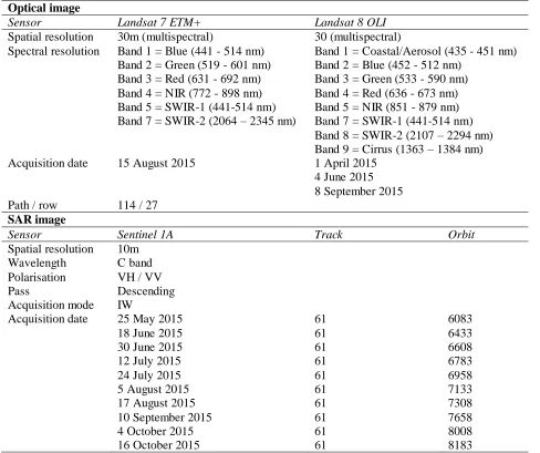
and that the dates of acquisition were within the rice-growing season (i.e., April to October). Four Landsat images free of cloud and snow contamination were available over the study site for 2015 (Table 2). With the available Landsat images, an NDVI image stack comprising four bands for each date was used as complementary phenology information in the classification experiments performed.
For this study, the available 12-day repeat cycle Sentinel-1A data covering the 2015 growing season from 25 May to 16 October 2015 was downloaded from the European Space Agency (ESA) Sentinels Scientific Data Hub website (https://scihub.copernicus.eu/classic/). The downloaded Sentinel-1A data were from a dual-polarisation radar, indicating that the system transmits and receives signals in both the horizontal (H) and vertical (V) polarisations. The dual polarisation SAR product allows measurement of polarisation properties for terrestrial surfaces, in addition to the backscatter intensity. The collection mode for the Sentinel-1A data used in this study was interferometric wide swath (IW), the primary operational mode over land. All downloaded SAR data used in the study were Ground Range Detected (GRDH), which meant the data had been detected, multi-looked and projected to the ground range using the World Geodetic System 1984 ellipsoidal model. The Level 1 GRDH products have the thermal noise removed to enhance the quality of the detected images. However, the Sentinel-1A products were not radiometrically corrected, thereby retaining radiometric bias, which necessitated image pre-processing. At the time of downloading, the dates listed in table 2 were the only available Sentinel-1A data covering the study area in 2015.
2.4. Training and validation data
The Jiansangjiang STB site provided a major source of land cover reference data for training and validation in the image classification experiments. This survey was complemented with additional land cover data extracted from fine spatial resolution Google Earth images dated 2012 to 2014. The land cover reference data were divided randomly in half for training and validation, respectively. In this study, four broad land cover classes were used during image classification. These classes were built-up areas (bare surfaces, industrial and commercial buildings, paved surfaces, roads, and fallow or open fields), non-rice fields (other crop species), vegetated (forest, wetlands, shrubs or plants with considerable density and height), and paddy rice fields.
Using the land cover reference data a total of 2000 points depicting the four broad land-cover classes were selected spatially randomly in a stratified manner. These point samples were used for accuracy assessment. For training of the satellite images to be classified, 464 polygons (each containing over 5000 pixels), depicting the target land-cover classes were digitised from the georeferenced fine-resolution Google Earth imagery. Considering that the paddy rice fields were the focus of the study, more training data depicting this class were extracted for the training process during image classification as adopted in Mansaray et al (2017).
2.5. Temporal backscatter profile of paddy rice fields
7
Table 2. Characteristics of optical and SAR data used in the study. Optical image
Sensor Landsat 7 ETM+ Landsat 8 OLI
Spatial resolution 30m (multispectral) 30 (multispectral)
Spectral resolution Band 1 = Blue (441 - 514 nm) Band 1 = Coastal/Aerosol (435 - 451 nm) Band 2 = Green (519 - 601 nm) Band 2 = Blue (452 - 512 nm)
Band 3 = Red (631 - 692 nm) Band 3 = Green (533 - 590 nm) Band 4 = NIR (772 - 898 nm) Band 4 = Red (636 - 673 nm) Band 5 = SWIR-1 (441-514 nm) Band 5 = NIR (851 - 879 nm) Band 7 = SWIR-2 (2064 – 2345 nm) Band 7 = SWIR-1 (441-514 nm)
Band 8 = SWIR-2 (2107 – 2294 nm) Band 9 = Cirrus (1363 – 1384 nm) Acquisition date 15 August 2015 1 April 2015
4 June 2015 8 September 2015 Path / row 114 / 27
SAR image
Sensor Sentinel 1A Track Orbit
Spatial resolution 10m Wavelength C band Polarisation VH / VV
Pass Descending
Acquisition mode IW
Acquisition date 25 May 2015 61 6083
18 June 2015 61 6433
30 June 2015 61 6608
12 July 2015 61 6783
24 July 2015 61 6958
5 August 2015 61 7133
17 August 2015 61 7308
10 September 2015 61 7658
4 October 2015 61 8008
16 October 2015 61 8183
2.6. Image pre-processing
2.6.1. Landsat imagery
8
relief displacements with only spacecraft ephemeris data. The downloaded Landsat images used in the study were L1T products. However, as a precutionary measure checks for geometric alignment for all input image datasets were performed as to ensure sufficiently accurate co-registration.
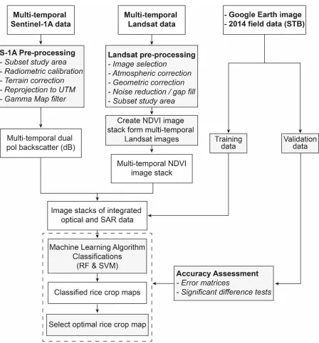
The Landsat image pre-processing stages included image selection, atmospheric correction, geometric correction of misaligned scenes, gap filling of Landsat 7 ETM+ images affected by failed Scan Line Correctors (SLC) and image sub-setting to include the study area (Figure 2). The Landsat images were atmospherically corrected to increase the quality of the images used for analysis. This correction was performed using atmospheric correction module FLAASH (Fast Line-of-sight Atmospheric Analysis of Spectral Hypercubes) in ENVI 5.3 (ENVI, 2016). All the bands of Landsat 7 ETM+ and Landsat 8 OLI images were atmospherically corrected using the FLAASH module. The downloaded Landsat metadata file contains descriptions of Level 1 data product characteristics and values for enhancing Landsat data (such as conversion to reflectance and radiance). All necessary information contained in the metadata file was used in the pre-processing of all downloaded Landsat data.
Geometric correction of misaligned Landsat images was performed using the polynomial geometric model in the ERDAS Imagine software (ERDAS, 2014). The Landsat 7 ETM+ image was affected by gaps resulting from SLC-off issues. The gaps were filled using the Landsat Gap fill pre-processing tool made available by ENVI (Yale Center for Earth Observation, 2013). The single file gap fill (triangulation) uses a linear transformation that adjusts the image based on the mean and standard deviation of each band contained in the scene (Scaramuzza et al., 2004).
After pre-processing, the red and NIR bands were used to calculate the NDVI images for all four dates downloaded. The NDVI has been applied widely in monitoring a variety of vegetation covers and is often used as a proxy for plant growth and productivity as the amount of solar radiation reflected off the vegetation canopy is related to wavelength, chlorophyll content, plant water content and canopy structure (Dong et al., 2015; Dorigo et al., 2012). NDVI was calculated using the formula:
𝑁𝐷𝑉𝐼 = (𝑁𝐼𝑅 − 𝑅𝑒𝑑)
(𝑁𝐼𝑅 + 𝑅𝑒𝑑) (1)
2.6.2. Sentinel-1A SAR data
The Sentinel-1A data were pre-processed using the Sentinel Application Platform (SNAP) open source software (http://step.esa.int/main/toolboxes/snap/). The pre-processing stages included radiometric calibration, range Doppler terrain correction, re-projection of the calibrated radar image to Universal Transverse Mercator (UTM) projection, and application of a speckle filter.
While uncalibrated Sentinel-1A SAR data may be sufficient for use in some circumstances, the process of SAR calibration is critical in harnessing the full information contained. The essence of SAR calibration is to provide imagery in which the pixel values could be related directly to radar backscatter of the scene. The conversion of SAR data to radiometrically-calibrated backscatter requires the use of metadata information downloaded with the Sentinel-1A data. The calibration process is realised by undoing the application output scaling and applying the desired scale. Using any of the four Look Up Tables (LUT) provided with level-1 products, the pixel values are returned as either of the following: sigma0 band ( ), gamma0 band ( ), beta0 band ( ) or the original DN band. Equation 2 shows the formula for radiometric calibration:
0
i
0
i
0
i
9
(2)
where, depending on the LUT = , , or original
The radiometrically corrected polarisation channels were then exported as sigma0 band values with unit dB. To compensate for geometric distortions introduced from the side-looking geometry of the images, the range Doppler terrain orthorectification was applied to radiometrically corrected Sentinel-1A images using the tools available in the SNAP software. The orthorectification algorithm uses the available metadata information on the orbit state vector, the radar timing annotations, slant to ground range conversion parameters and a reference digital elevation model dataset to derive the precise geolocation information. The orthorectified SAR image was further resampled to a spatial resolution of 10 m using bilinear interpolation and re-projected to the Universal Transverse Mercator system Zone 53 North, WGS 84.
After orthorectification, the presence of granular noise in the form of speckles across SAR images was removed using the Gamma-MAP (Maximum A Posteriori) filter (Frost et al., 1982; Mansourpour et al., 2006). The Gamma-MAP filter is a multiplicative noise model with non-stationary mean and variance parameters (Frost et al., 1982). In this study, a 7x7-gamma map filter with three looks (Chen et al., 2007) was applied to all the Sentinel-1A images.
2.7. Machine learning algorithms: SVM & RF
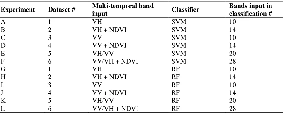
As presented in figure 2, different combinations of multi-temporal polarisation bands and Landsat-derived NDVI time-series data were used for the image classification experiments. Table 3 summarises the fused multi-temporal SAR and NDVI datasets used in classification experiments. The machine learning algorithms evaluated were the SVM and RF. SVM and RF classifiers are known to be capable of producing significantly higher classification accuracy in comparison to traditional classifiers, such as the maximum likelihood classifier, while using a limited number of training samples. The SVM and RF classifications were performed using the Segmentation and Classification tool in ESRI ArcGIS 10.4 Desktop application
[image:9.596.77.532.522.704.2](www.esri.com).
Table 3. Fused multi-temporal Sentinel-1A SAR and Landsat NDVI time-series used in study. Experiment Dataset # Multi-temporal band
input Classifier
Bands input in classification #
A 1 VH SVM 10
B 2 VH + NDVI SVM 14
C 3 VV SVM 10
D 4 VV + NDVI SVM 14
E 5 VH/VV SVM 20
F 6 VV/VH + NDVI SVM 28
G 1 VH RF 10
H 2 VH + NDVI RF 14
I 3 VV RF 10
J 4 VV + NDVI RF 14
K 5 VH/VV RF 20
L 6 VV/VH + NDVI RF 28
2 2 i i i DN value A i value 0 i 0 i 0 i
10
Figure 2. Framework for combining multi-temporal SAR and NDVI data for rice crop mapping in the study area.
2.7.1. Support Vector Machine
11
minimization (Mountrakis et al., 2011). Under this system, SVMs minimise classification error on unseen data without prior assumptions made on the probability distribution of the data. One advantage of SVMs is that they are relatively insensitive to training sample size and can be used with limited quantity and quality of training samples (Mountrakis et al., 2011). This ability to generalise well from a limited amount and/or quality of training data makes SVMs a well-used machine-learning algorithm in remote sensing. In contrast to alternative classification models such as neural networks, SVMs offer additional benefits. The SVM model supports multiple kernels, including the popular linear and radial basis function (RBF) kernels. A major challenge of using the SVM is the choice of kernel. Mountrakis et al. (2011) observed that although numerous options are available for kernel selection in SVMs some of these might not be optimal for remote sensing. As demonstrated in Zhu and Blumberg (2002), the RBF and polynomial kernels applied in the SVM-based classification of satellite sensor image data produced different results. In this study, we tested the RBF and polynomial kernels of the SVM in order to establish the best model for the input datasets.
2.7.2. Random Forest
The RF is a decision tree ensemble classifier proposed by Breiman (2001) which is built to handle high data dimensionality effectively and has demonstrated to be an improvement over traditional decision trees (Immitzer et al., 2012). The RF algorithm consists of a collection of tree-based classifiers. Each decision tree is constructed using a deterministic algorithm by a bootstrap, leaving the remaining data points for validation and casts a unit vote for the most popular class. To enhance the diversity of the classification trees, RF uses the bootstrapping procedure with replacement to allocate each pixel to a class in accordance with the maximum number of votes from the collection of trees (Son et al., 2017). The Gini index is used to define splitting thresholds and is a measure of the child node class homogeneity relative to the distribution of classes in the parent node (Balzter et al., 2015). The RF algorithm allows analysis of the variable importance with the Gini coefficient with a range of 0 to 1 depicting completely homogeneous and completely heterogeneous, respectively. The key parameters required to define the RF are the number of decision trees to create (k) and the number of randomly selected variables (m) considered for splitting each node in a tree. Several studies have investigated the use of RF for classifying SAR datasets (Balzter et al., 2015; Fu et al., 2017; Son et al., 2017).
2.8. Accuracy assessment
Using the error matrices, accuracies of the SVM and RF classified images were calculated. The performance of the classified outputs was further assessed using the overall classification accuracy, producer’s accuracy, user’s accuracy, and Kappa statistic. A test for levels of significant difference for all classifications was assessed using the McNemar’s test (Agresti, 1996; Bradley, 1968) as implemented in recent vegetation analysis studies (Onojeghuo and Onojeghuo, 2017; Son et al., 2017). The McNemar’s test is a non-parametric test applied to generated confusion matrices that have a 2x2 dimension. The test is based on the standardised normal statistic z:
𝑧 = (𝑓12− 𝑓21) √(𝑓12+ 𝑓21)
(3)
where f12 and f21 are the off-diagonal entries in the matrix. The classification accuracies are
12
3. Results
3.1. Interpretation of paddy rice backscatter temporal profile
13
Figure 3. Temporal backscatter profiles of paddy rice fields for both polarisations (VH and VV) of Sentinel-1A imagery acquired within the 2015 rice-growing season for selected sites in Jiansanjiang, Sanjiang Plain, Heilongjiang Province, China.
3.2. SVM classification results
14
significantly increased by approximately 17% and 8%, respectively (Table 4). Both SVM based experiments (i.e. B v. C and E v. F) had increases in the overall accuracies that were significant at the 99% level with Z-score values of 18.7 and 12.6, respectively (Table 5). The inclusion of NDVI time-series as complementary information in the classifications substantially increased the overall classification accuracies (Mansaray et al., 2017; Torbick et al., 2017). However, with the inclusion of NDVI data the paddy rice class accuracies experienced a significant decline, a result similar to Mansaray et al. (2017). The accuracy results showed that for the paddy rice class, the Kappa statistic declined from 0.86 to 0.85 when the NDVI time-series data was added to the VH polarisation data (Table 4, Table 5 – A v. B). Similarly, paddy rice Kappa statistic values for VV and VH/VV polarisations integrated with NDVI time-series significantly declined from 0.83 to 0.77 (Table 5, significant difference at 95% level for experiments C v. D) and 0.89 to 0.82 (Table 5, significant difference at 95% level for experiments E v. F).
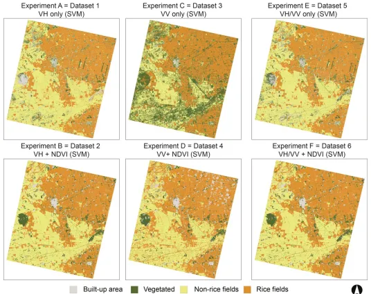
Results of the SVM classifications presented in Table 6 indicate that the per-class accuracies were not completely even in identifying each land-cover class. The user’s accuracy (UA) for the paddy rice class declined from 89.8% in experiment A to 88.5% in experiment B (Table 6). In a similar manner, the UA of the paddy rice class for experiments C and D declined from 87.5% to 82.9%. For the multi-temporal dual polarisation dataset (dataset 5), UA for experiment E declined from 91.6% to 86.4% when NDVI time-series data was introduced in the SVM classification process. However, of all the SVM-based classifications the highest accuracy for the paddy rice class was generated in experiment E (i.e dataset 5 dual polarisation bands - VH/VV) with a UA of 91.6%. Results of the McNemar’s test revealed that for the paddy rice class the result of experiment E was significantly higher than experiments B, C, D, and F with the exception of experiment A (which had a Z-score of 1, Table 5). Hence, for the SVM-based classifications the optimal dataset was identified as dataset 5 (experiment E, with overall classification accuracy = 82.5%, overall Kappa = 0.77, and paddy rice Kappa = 0.89 – Table 4). Figure 4 presents the SVM classified maps generated using a combination of multi-temporal Sentinel-1A SAR data and NDVI time-series images.
3.3. RF classification results
To execute RF image classification the number of trees and number of predictors are vital parameter settings required to maximise the model accuracy. Several tests to determine the best number of trees (k) needed for implementing RF classification were undertaken using values within the range of 50 to 300 at an interval of 50. The k value equal to 100 produced the highest classification accuracy for paddy rice classification. All RF-based experiments in this study had their settings made to 50. The maximum number of tree depth and samples per class were set to 30 and 1000, respectively.
15
However, unlike the SVM classifications, the accuracy of the paddy rice class in the RF classifications increased significantly when the single and dual polarisation channels were fused with NDVI time-series in the classification process. The paddy rice UA of experiment G increased from 91.7% to 95% (experiment H) when NDVI time-series data were introduced. Similarly, UA of experiments I and K increased from 91.3% to 93.8% in experiment J and 92.4% to 94.8% in experiment L, respectively. Results of the McNemar’s test showed a significant improvement in paddy rice classification accuracy when the NDVI time-series was integrated with dataset 1 (multi-temporal VH polarisation) and dataset 3 (multi-temporal VV polarisation) with Z-scores of 2 and 2.65, respectively (Table 5, experiments G v. H and I v. J). For the paddy rice class, the experiments that generated the highest UA were experiments H (dataset 2 - VH) and L (dataset 6 - VH/VV + NDVI) both having 96.7% (Table 7). In a similar manner, the highest overall classification accuracies were for experiments H (Table 4, 95.2%) and L (Table 4, 95.3%), respectively. Results of the McNemar’s test for significant difference indicated that for the paddy rice class and overall class there was no significant difference in the results (Table 5, H v. L for overall and paddy rice class). In terms of practical use and computational needs, dataset 2 (i.e. VH + NDVI, 14 bands) was a better option for mapping in comparison to dataset 6 (i.e. VH/VV + NDVI, 28 bands). Hence, the optimal dataset for paddy rice mapping based on the RF classifier was dataset 2 (i.e. VH + NDVI, 14 bands). Figure 5 presents the RF classified maps generated using a combination of multi-temporal SAR and NDVI images.
3.4. Comparison of optimal SVM and RF classified outputs
[image:15.596.82.497.602.787.2]Based on the classification results in the previous sections, the optimal SVM and RF classified results were produced in experiment E (dataset 2 - VH/VV) and experiment H (dataset 2 – VH + NDVI). The overall classification accuracy of RF-based experiment H was 12.7% higher than the SVM classified output (experiment E), a significant difference at the 99% level. For the paddy rice class the SVM classification significantly declined in accuracy (user’s accuracy, producer’s accuracy, and Kappa statistic) when NDVI data were included in the process, results consistent with Mansaray et al. (2017). For the RF classification, there was a substantial increase in paddy rice classification accuracy when the NDVI images were integrated into the classification process (Table 7, Table 5 – G v. H and I v. J). For the paddy rice class, the user’s accuracy and Kappa statistic of the RF-based experiment H (Tables 4 and 7, 95% and 0.93) were significantly higher than the optimal SVM-based experiment E (Tables 4 and 7, 0.89 and 91.6%). Figure 6 shows the optimal SVM and RF classified outputs generated in the study.
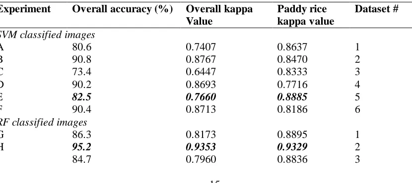
Table 4. Classification accuracy results of Support Vector Machine and Random Tree classifications (best results in bold italic).
Experiment Overall accuracy (%) Overall kappa Value
Paddy rice kappa value
Dataset #
SVM classified images
A 80.6 0.7407 0.8637 1
B 90.8 0.8767 0.8470 2
C 73.4 0.6447 0.8333 3
D 90.2 0.8693 0.7716 4
E 82.5 0.7660 0.8885 5
F 90.4 0.8713 0.8186 6
RF classified images
G 86.3 0.8173 0.8895 1
H 95.2 0.9353 0.9329 2
16
Experiment Overall accuracy (%) Overall kappa Value
Paddy rice kappa value
Dataset #
J 95.3 0.9373 0.9179 4
K 89.9 0.8647 0.8990 5
[image:16.596.76.554.203.681.2]L 95.3 0.9367 0.9304 6
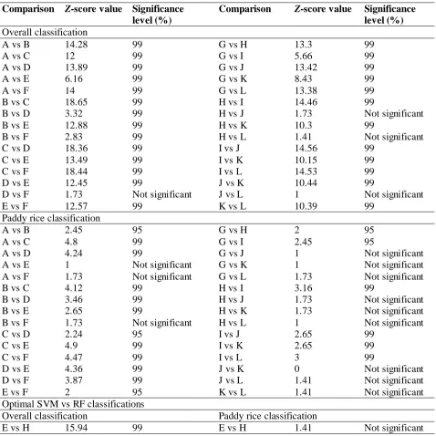
Table 5. Results of McNemar’s test for significant differences in overall and paddy rice accuracies for SVM and RF classified outputs.
Comparison Z-score value Significance level (%)
Comparison Z-score value Significance level (%) Overall classification
A vs B 14.28 99 G vs H 13.3 99
A vs C 12 99 G vs I 5.66 99
A vs D 13.89 99 G vs J 13.42 99
A vs E 6.16 99 G vs K 8.43 99
A vs F 14 99 G vs L 13.38 99
B vs C 18.65 99 H vs I 14.46 99
B vs D 3.32 99 H vs J 1.73 Not significant
B vs E 12.88 99 H vs K 10.3 99
B vs F 2.83 99 H vs L 1.41 Not significant
C vs D 18.36 99 I vs J 14.56 99
C vs E 13.49 99 I vs K 10.15 99
C vs F 18.44 99 I vs L 14.53 99
D vs E 12.45 99 J vs K 10.44 99
D vs F 1.73 Not significant J vs L 1 Not significant
E vs F 12.57 99 K vs L 10.39 99
Paddy rice classification
A vs B 2.45 95 G vs H 2 95
A vs C 4.8 99 G vs I 2.45 95
A vs D 4.24 99 G vs J 1 Not significant
A vs E 1 Not significant G vs K 1 Not significant
A vs F 1.73 Not significant G vs L 1.73 Not significant
B vs C 4.12 99 H vs I 3.16 99
B vs D 3.46 99 H vs J 1.73 Not significant
B vs E 2.65 99 H vs K 1.73 Not significant
B vs F 1.73 Not significant H vs L 1 Not significant
C vs D 2.24 95 I vs J 2.65 99
C vs E 4.9 99 I vs K 2.65 99
C vs F 4.47 99 I vs L 3 99
D vs E 4.36 99 J vs K 0 Not significant
D vs F 3.87 99 J vs L 1.41 Not significant
E vs F 2 95 K vs L 1.41 Not significant
Optimal SVM vs RF classifications
Overall classification Paddy rice classification
17
Table 6. Error matrix of SVM classified outputs (where BU=Built-up, VG=Vegetated, NRC=Non-rice crops, PR=Paddy rice, PA=Producer’s accuracy, and UA=Users accuracy). Best results in bold italic.
VH Reference data VV+NDVI Reference data
Classified
data BU VG NRC PR
Row total PA (%) UA (%) Classified
data BU VG NRC PR
Row total PA (%) UA (%)
BU 277 29 29 2 337 55.4 82.2 BU 439 12 10 8 469 87.8 93.6
VG 140 421 40 1 602 84.2 69.9 VG 14 449 16 2 481 89.8 93.4
NRC 67 20 421 5 513 84.2 82.1 NRC 10 10 442 16 478 88.4 92.5
PR 16 30 10 492 548 98.4 89.8 PR 37 29 32 474 572 94.8 82.9
Column
total 500 500 500 500 1611
Column
total 500 500 500 500 1804
VH + NDVI Reference data VH/VV Reference data
Classified
data BU VG NRC PR
Row total
PA (%)
UA
(%) Classified data BU VG NRC PR
Row total PA (%) UA (%)
BU 433 4 14 1 452 86.6 95.8 BU 300 23 28 1 352 60 85.2
VG 16 458 30 5 509 91.6 90 VG 111 430 40 3 584 86 73.6
NRC 30 14 438 8 490 87.6 89.4 NRC 75 22 426 3 526 85.2 81
PR 21 24 18 486 549 97.2 88.5 PR 14 25 6 493 538 98.6 91.6
Column
total 500 500 500 500 1815
Column
total 500 500 500 500 1649
VV Reference data VH/VV+NDVI Reference data
Classified
data BU VG NRC PR
Row total
PA (%)
UA
(%) Classified data BU VG NRC PR
Row total PA (%) UA (%)
BU 211 0 2 0 213 42.2 99.1 BU 427 4 12 1 444 85.4 96.2
VG 174 421 125 25 745 84.2 56.5 VG 16 456 30 5 507 91.2 89.9
NRC 89 45 366 6 506 73.2 72.3 NRC 28 15 435 5 483 87 90.1
PR 26 34 7 469 536 93.8 87.5 PR 29 25 23 489 566 97.8 86.4
Column
total 500 500 500 500 1467
Column
18
Table 7. Error matrix of RF classified outputs (where BU=Built-up, VG=Vegetated, NRC=Non-rice crops, PR=Paddy rice, PA=Producer’s accuracy, and UA=Users accuracy). Best results in bold italic.
VH Reference data VV+NDVI Reference data
Classified
data BU VG NRC PR
Row total PA (%) UA (%) Classified
data BU VG NRC PR
Row total PA (%) UA (%)
BU 376 51 27 7 461 75.2 81.6 BU 480 6 13 7 506 96 94.9
VG 73 412 17 0 502 82.4 82.1 VG 10 468 15 1 494 93.6 94.7
NRC 37 12 451 6 506 90.2 89.1 NRC 4 2 470 4 480 94 97.9
PR 14 25 5 487 531 97.4 91.7 PR 6 24 2 488 520 97.6 93.8
Column
Total 500 500 500 500 1726
Column
total 500 500 500 500 1906
VH + NDVI Reference data VH/VV Reference data
Classified
data BU VG NRC PR
Row total
PA (%)
UA
(%) Classified data BU VG NRC PR
Row total PA (%) UA (%)
BU 471 8 14 5 498 94.2 94.6 BU 417 42 17 7 483 83.4 86.3
VG 15 472 12 1 500 94.4 94.4 VG 39 427 15 0 481 85.4 88.8
NRC 11 2 469 3 485 93.8 96.7 NRC 30 8 465 5 508 93 91.5
PR 3 18 5 491 517 98.2 95 PR 14 23 3 488 528 97.6 92.4
Column
Total 500 500 500 500 1903
Column
total 500 500 500 500
VV Reference data VH/VV+NDVI Reference data
Classified
data BU VG NRC PR
Row total
PA (%)
UA
(%) Classified data BU VG NRC PR
Row total PA (%) UA (%)
BU 373 43 29 9 454 74.6 82.2 BU 472 6 13 7 498 94.4 94.8
VG 71 411 40 3 525 82.2 78.3 VG 13 470 12 1 496 94 94.8
NRC 40 18 429 7 494 85.8 86.8 NRC 11 3 473 2 489 94.6 96.7
PR 16 28 2 481 527 96.2 91.3 PR 4 21 2 490 517 98 94.8
Column
Total 500 500 500 500 1694
Column
19
20
21
22
4. Discussion
The results of this study demonstrate the contribution that Sentinel-1A data can towards delivering crop monitoring systems that operate at fine spatio-temporal resolutions, potentially across regional and global scales (Dong et al., 2015; Mansaray et al., 2017; Nguyen et al., 2016; Shao et al., 2016; Torbick et al., 2017). We employed multi-temporal Sentinel-1 GRDH images and Landsat-derived NDVIs for the 2015 rice-growing season to map paddy rice fields with two machine-learning algorithms – SVM and RF. The radar and multispectral imagery used spanned over the pre-planting / flooding stage to the heading/dough stages of paddy rice, a period at which changes in temporal backscatter of rice are most prominent (Mansaray et al., 2017). Although single-season rice cultivation is common practice in the study area, a large level of inter-field variability in the growth of rice crops is still present, owing to the difference in planting dates and varieties. Toan et al. (1997) noted that in a single-season rice cultivation system, planting dates between adjacent fields could vary up to eight weeks in certain parts of China. In addition to varied planting dates, the influences of varied management practices across fields can lead to remarkable differences in crop growth performance. Thus, the use of single-date SAR (or other) imagery for paddy rice mapping is very limiting and this necessitates the use of multi-temporal data.
In addition to multi-temporal microwave satellite sensor data, the inclusion of optically-derived VIs (such as NDVI time-series) depicting crop phenological information can facilitate more accurate methods of discriminating paddy rice fields from adjoining land-cover classes. As demonstrated in this study, we evaluated the performance of different combinations of multi-temporal single and dual polarisation SAR channels with NDVI time-series images using two machine learning algorithms. The accuracy assessment results for both the SVM- and RF-based classifiers revealed a significant increase in the overall classification accuracy when the NDVI time-series data were integrated with the SAR data. Considering accuracy of the paddy rice class specifically, results of the SVM and RF classifications, revealed the optimal inputs were dataset 5 (for SVM experiment E, paddy rice Kappa = 0.89 – Table 4) and dataset 2 (for RF experiment H, paddy rice Kappa = 0.93 – Table 4). While classification accuracy for rice was higher with RF than SVM, the difference was not statistically significant. However, similar studies have shown that RF classifiers usually outperform SVMs in varied land cover mapping related projects (Onojeghuo and Onojeghuo, 2017; Son et al., 2017). The results of the present study also demonstrated that when multi-temporal single (VH and VV) and dual (VH/VV) polarisation SAR bands are integrated with NDVI data there was a significant increase in rice field classification accuracy (Dong et al., 2015; Mansaray et al., 2017).
Although the inclusion of NDVI data significantly increased the overall classification accuracy, for the paddy rice class the effect varied according to the classification algorithm. The NDVI data increased the rice class accuracy with the RF algorithm but decreased the accuracy with the SVM. With the RF -based approach the NDVI time-series data assisted in removing the influence of water bodies and built-up pixels in the classifications, results similar to those obtained by Mansaray et al. (2017).
5. Conclusion
23
The classified outputs generated with both classifiers showed a significant increase in the overall classification accuracies when NDVI data were introduced to the classification process. The results showed that the optimal approach with the best overall and paddy rice classification accuracy was the VH polarisation SAR data combined with NDVI time series (i.e. dataset 2 = VH + NDVI) classified using the RF algorithm. This approach achieved paddy rice and overall Kappa values of 0.94 and 0.93, respectively. The paddy rice user’s accuracy and overall classification accuracy was 96.7% and 95.2%, respectively. The results of the study further validate the relevance of the RF classification approach to monitoring the spatiotemporal dynamics of paddy rice fields.
A step forward from this study would be to implement the RF-approach on operational basis producing fine spatial resolution paddy rice field maps based on Sentinel-1A SAR data combined with additional NDVI-based phenological information. In addition, either of the evaluated classifiers could be implemented with limited ground training data making the use of machine learning algorithms a cost-effective, fast, and robust approach compared to other traditional pixel-based classifiers such as maximum likelihood algorithms. In the absence of optically-derived phenological information, the study further demonstrates the relevance of utilising both multi-temporal polarisation channels (VH and VV) in the classification process with either the SVM or RF machine learning algorithms. Hence, the growing repository of open access, frequent multi-temporal SAR data provided by the Sentinel-1A and 1B satellites holds considerable promise as the basis for rice crop mapping from regional to global scales.
Acknowledgement
The authors would like to thank the graduate students from China Agricultural University for their contribution to conducting field surveys at the study site. The UK Science and Technology Facilities Council (STFC) Newton Agri-Tech programme financially supported this research, under project “Remote Sensing for Sustainable Intensification in China”.
References
Agresti, A., 1996. An introduction to Categorical Data Analysis. Wiley, New York, N.Y.
Balzter, H., Cole, B., Thiel, C., Schmullius, C., 2015. Mapping CORINE land cover from Sentinel-1A SAR and SRTM digital elevation model data using Random Forests. Remote Sensing 7, 14876-14898. Becker-Reshef, I., Justice, C., Sullivan, M., Vermote, E., Tucker, C., Anyamba, A., Small, J., Pak, E., Masuoka, E., Schmaltz, J., Hansen, M., Pittman, K., Birkett, C., Williams, D., Reynolds, C., Doorn, B., 2010. Monitoring Global Croplands with Coarse Resolution Earth Observations: The Global Agriculture Monitoring (GLAM) Project. Remote Sensing 2, 1589.
Bouvet, A., Le Toan, T., Lam-Dao, N., 2009. Monitoring of the rice cropping system in the Mekong Delta using ENVISAT/ASAR dual polarisation data. IEEE Transactions on Geoscience and Remote Sensing 47, 517-526.
Bradley, J.V., 1968. Distribution-Free Statistical Test. Prentice-Hall, Englewood Cliffs, New Jersy. Breiman, L., 2001. Random forests. Machine Learning 45, 5-32.
Chen, C., McNairn, H., 2006. A neural network integrated approach for rice crop monitoring. International Journal of Remote Sensing 27, 1367-1393.
Chen, J., Huang, J., Hu, J., 2011a. Mapping rice planting areas in southern China using the China Environment Satellite data. Mathematical and Computer Modelling 54, 1037-1043.
Chen, J., Lin, H., Pei, Z., 2007. Application of ENVISAT ASAR data in mapping rice crop growth in Southern China. IEEE Geoscience and Remote Sensing Letters 4, 431-435.
24
Cheng, Y., Wang, X., Guo, J., Zhao, Y.-x., Huang, J.-f., 2012. The temporal–spatial dynamic analysis of China rice production. Scientia Agricultura Sinica 45, 3473-3485.
China Import Export, 2014. China Rice Imports Reach Record High. China Import Export.
Clauss, K., Yan, H., Kuenzer, C., 2016. Mapping Paddy Rice in China in 2002, 2005, 2010 and 2014 with MODIS Time Series. Remote Sensing 8, 434.
Ding, C., 2003. Land policy reform in China: assessment and prospects. Land use policy 20, 109-120. Dong, J., Xiao, X., Kou, W., Qin, Y., Zhang, G., Li, L., Jin, C., Zhou, Y., Wang, J., Biradar, C., 2015. Tracking the dynamics of paddy rice planting area in 1986–2010 through time series Landsat images and phenology-based algorithms. Remote Sensing of Environment 160, 99-113.
Dorigo, W., Jeu, R.d., Chung, D., Parinussa, R., Liu, Y., Wagner, W., Fernández‐Prieto, D., 2012. Evaluating global trends (1988–2010) in harmonized multi‐satellite surface soil moisture. Geophysical Research Letters 39.
ENVI, 2016. ENVI Geospatial Solutions. Harris Geospatial Solutions.
ERDAS, 2014. ERDAS Imagine 2014, 2014 ed. Hexagon Geospatial, Peachtree Corners Circle Norcross.
Ewing, J.J., Zhang, H., 2013. China as the World’s Largest Rice Importer: Regional Implications, in: reliefweb (Ed.).
Fan, W., Chao, W., Hong, Z., Bo, Z., Yixian, T., 2011. Rice Crop Monitoring in South China With RADARSAT-2 Quad-Polarization SAR Data. Geoscience and Remote Sensing Letters, IEEE 8, 196-200.
FAOSTAT, 2014. Statistical Database of the Food and Agricultural Organization of the United Nations. Foody, G.M., Mathur, A., 2004. A relative evaluation of multiclass image classification by support vector machines. IEEE Transactions on Geoscience and Remote Sensing 42, 1335-1343.
Fred, G., Hansen, J., Jewison, M., 2014. China’s Growing Demand for Agricultural Imports, U.S. Department of Agriculture, Economic Research Service.
Frost, V.S., Stiles, J.A., Shanmugan, K.S., Holtzman, J.C., 1982. A model for radar images and its application to adaptive digital filtering of multiplicative noise. IEEE Transactions on Pattern Analysis and Machine Intelligence, 2, 157-166.
Fu, B., Wang, Y., Campbell, A., Li, Y., Zhang, B., Yin, S., Xing, Z., Jin, X., 2017. Comparison of object-based and pixel-based Random Forest algorithm for wetland vegetation mapping using high spatial resolution GF-1 and SAR data. Ecological Indicators 73, 105-117.
Gnyp, M.L., Miao, Y., Yuan, F., Ustin, S.L., Yu, K., Yao, Y., Huang, S., Bareth, G., 2014. Hyperspectral canopy sensing of paddy rice aboveground biomass at different growth stages. Field Crops Research 155, 42-55.
Huang, Q., Zhang, L., Wu, W., Li, D., 2010. MODIS-NDVI-Based crop growth monitoring in China Agriculture Remote Sensing Monitoring System, Geoscience and Remote Sensing (IITA-GRS), 2010 Second IITA International Conference on, pp. 287-290.
Immitzer, M., Atzberger, C., Koukal, T., 2012. Tree Species Classification with Random Forest Using Very High Spatial Resolution 8-Band WorldView-2 Satellite Data. Remote Sensing 4, 2661.
Inoue, Y., Kurosu, T., Maeno, H., Uratsuka, S., Kozu, T., Dabrowska-Zielinska, K., Qi, J., 2002. Season-long daily measurements of multifrequency (Ka, Ku, X, C, and L) and full-polarization backscatter signatures over paddy rice field and their relationship with biological variables. Remote Sensing of Environment 81, 194-204.
Inoue, Y., Sakaiya, E., Wang, C., 2014. Capability of C-band backscattering coefficients from high-resolution satellite SAR sensors to assess biophysical variables in paddy rice. Remote Sensing of Environment 140, 257-266.
IRRI, 2016. Important management factors by growth stage. International Rice Research Institute (IRRI),.
Jin, C., Xiao, X., Dong, J., Qin, Y., Wang, Z., 2016. Mapping paddy rice distribution using multi-temporal Landsat imagery in the Sanjiang Plain, northeast China. Frontiers of Earth Science 10, 49-62. Kuenzer, C., Knauer, K., 2013. Remote sensing of rice crop areas. International Journal of Remote Sensing 34, 2101-2139.
25
Kussul, N., Skakun, S., Shelestov, A., Kussul, O., 2014. The use of satellite SAR imagery to crop classification in Ukraine within JECAM project, Geoscience and Remote Sensing Symposium (IGARSS), 2014 IEEE International. IEEE, pp. 1497-1500.
Le Toan, T., Ribbes, F., Li-Fang, W., Floury, N., Kung-Hau, D., Jin Au, K., Fujita, M., Kurosu, T., 1997. Rice crop mapping and monitoring using ERS-1 data based on experiment and modeling results. IEEE Transactions on Geoscience and Remote Sensing 35, 41-56.
Liu, J., Kuang, W., Zhang, Z., Xu, X., Qin, Y., Ning, J., Zhou, W., Zhang, S., Li, R., Yan, C., Wu, S., Shi, X., Jiang, N., Yu, D., Pan, X., Chi, W., 2014. Spatiotemporal characteristics, patterns, and causes of land-use changes in China since the late 1980s. Journal of Geographical Sciences 24, 195-210. Mansaray, L.R., Huang, W., Zhang, D., Huang, J., Li, J., 2017. Mapping Rice Fields in Urban Shanghai, Southeast China, Using Sentinel-1A and Landsat 8 Datasets. Remote Sensing 9, 257.
Mansourpour, M., Rajabi, M., Blais, J., 2006. Effects and performance of speckle noise reduction filters on active radar and SAR images, ISPRS Volume Number: XXXVI-I W: Topographic Mapping fro m Space (with Special Emphasis on Small Satellites), Ankara, Turkey
Mantero, P., Moser, G., Serpico, S.B., 2005. Partially supervised classification of remote sensing images through SVM-based probability density estimation. IEEE Transactions on Geoscience and Remote Sensing 43, 559-570.
McNairn, H., Champagne, C., Shang, J., Holmstrom, D., Reichert, G., 2009. Integration of optical and Synthetic Aperture Radar (SAR) imagery for delivering operational annual crop inventories. ISPRS Journal of Photogrammetry and Remote Sensing 64, 434-449.
Mosleh, M.K., Hassan, Q.K., Chowdhury, E.H., 2015. Application of remote sensors in mapping rice area and forecasting its production: A review. Sensors 15, 769-791.
Mountrakis, G., Im, J., Ogole, C., 2011. Support vector machines in remote sensing: A review. ISPRS Journal of Photogrammetry and Remote Sensing 66, 247-259.
NASA Goddard Space Flight Center, 2011. Landsat 7 science data users handbook. http://landsathandbook.gsfc.nasa.gov/pdfs/Landsat7_Handbook.pdf.
Nguyen, D.B., Gruber, A., Wagner, W., 2016. Mapping rice extent and cropping scheme in the Mekong Delta using Sentinel-1A data. Remote Sensing Letters 7, 1209-1218.
Onojeghuo, A.O., Onojeghuo, A.R., 2017. Object-based habitat mapping using very high spatial resolution multispectral and hyperspectral imagery with LiDAR data. International Journal of Applied Earth Observation and Geoinformation 59, 79-91.
Oyoshi, K., Tomiyama, N., Okumura, T., Sobue, S., 2013. Asia Rice Crop Estimation and Monitoring (Asia-RiCE) for GEOGLAM, AGU Fall Meeting Abstracts.
Scaramuzza, P., Micijevic, E., Chander, G., 2004. SLC gap-filled products phase one methodology. Landsat Technical Notes.
Science and Technology Backyard, 2017. What is Science&Technology Backyard?
Shao, Z., Fu, H., Fu, P., Yin, L., 2016. Mapping Urban Impervious Surface by Fusing Optical and SAR Data at the Decision Level. Remote Sensing 8, 945.
Smil, V., 1999. China's agricultural land. The China Quarterly 158, 414-429.
Son, N.T., Chen, C.F., Chen, C.R., Minh, V.Q., 2017. Assessment of Sentinel-1A data for rice crop classification using random forests and support vector machines. Geocarto International, 1-15.
Tan, M., Li, X., Xie, H., Lu, C., 2005. Urban land expansion and arable land loss in China—a case study of Beijing–Tianjin–Hebei region. Land use policy 22, 187-196.
Tao, F., Yokozawa, M., Liu, J., Zhang, Z., 2009. Climate change, land use change, and China’s food security in the twenty-first century: an integrated perspective. Climatic Change 93, 433-445.
Teng, F., Chen, Z.X., Wu, W.B., Huang, Q., Li, D.D., Tian, X., 2012. Yield estimation of winter wheat in North China Plain by using crop growth monitoring system (CGMS), Agro -Geoinformatics (Agro-Geoinformatics), 2012 First International Conference on, pp. 1-4.
Torbick, N., Chowdhury, D., Salas, W., Qi, J., 2017. Monitoring Rice Agriculture across Myanmar Using Time Series Sentinel-1 Assisted by Landsat-8 and PALSAR-2. Remote Sensing 9, 119.
Vapnik, V.N., Vapnik, V., 1998. Statistical Learning Theory. Wiley New York.
Wang, F.-M., Huang, J.-F., Wang, X.-Z., 2008. Identification of Optimal Hyperspectral Bands for Estimation of Rice Biophysical Parameters. Journal of Integrative Plant Biology 50, 291-299.
26
Yale Center for Earth Observation, 2013. Filling Gaps in Landsat ETM Images.
Yang, H., Li, X., 2000. Cultivated land and food supply in China. Land use policy 17, 73-88.
Zhang, G., Xiao, X., Dong, J., Kou, W., Jin, C., Qin, Y., Zhou, Y., Wang, J., Menarguez, M.A., Biradar, C., 2015. Mapping paddy rice planting areas through time series analysis of MODIS land surface temperature and vegetation index data. ISPRS Journal of Photogrammetry and Remote Sensing 106, 157-171.
Zhang, Y., Wang, Y., Su, S., Li, C., 2011. Quantifying methane emissions from rice paddies in Northeast China by integrating remote sensing mapping with a biogeochemical model. Biogeosciences 8, 1225.