A Markov state modeling approach to
characterizing the punctuated equilibrium
dynamics of stochastic evolutionary games
M. Hallier
∗, C. Hartmann
†February 15, 2016
Abstract
Stochastic evolutionary games often share a dynamic property called punctuated equilibrium; this means that their sample paths exhibit long periods of stasis near one population state which are infrequently inter-rupted by switching events after which the sample paths stay close to a different population state, again for a long period of time. This has been described in the literature as a favorable property of stochastic evolu-tionary games. The methods used so far in stochastic evoluevolu-tionary game theory, however, do not fully characterize these dynamics. We present an approach that aims at exposing the punctuated equilibrium dynamics by constructing Markov models on a reduced state space which approximate well this dynamic behavior. Besides having good approximation proper-ties, the approach allows a simulation-based algorithm, which is appealing in the case of complex games.
∗Free University Berlin, Berlin, Germany †Free University Berlin, Berlin, Germany
1
Introduction
Stochastic evolutionary games often share the punctuated equilibrium property; this means that their sample paths exhibit long periods of stasis near one pop-ulation state which are infrequently interrupted by switching events after which the sample paths stay close to a different population state, again for a long period of time. This punctuated equilibrium property has been characterized in the literature as a favorable property of stochastic evolutionary games (e.g., Young, 1998, 2006), not least because it might lead to a different perspective on modeling conventions and on the problem of equilibrium selection (Jaeger, 2008, 2012).
The methods used so far in stochastic evolutionary game theory, however, do not characterize the dynamics of the evolutionary games with respect to this property. More specifically, the analysis of evolutionary game models exclusively focuses on equilibrium selection, equilibria of mean dynamics, or the determi-nation of stochastically stable states (Benaim and Weibull, 2003; Ellison, 2000; Foster and Young, 1990; Hofbauer and Sigmund, 2003; Kurtz, 1970; Sandholm, 2010, 2011; Weibull, 1995; Young, 1993, 1998, 2006). All of these approaches are not able to thorougly describe punctuated equilibrium dynamic behavior of the considered evolutionary processes.
This is in contrast to physics and chemistry where there has been much research in the last century on the mathematical description and analysis of this dynamic property1(for a short historical overview see, e.g., the introductory
chapter of Bovier, 2009). We build on these existing approaches to present a novel approach to the analysis of stochastic evolutionary games. In particular, after introducing the necessary game theoretical notions (Section 2), we show how to construct Markov models of reduced complexity that approximate their essential dynamic behavior (Section 3). The basic idea behind these so-called
Markov state modelsis to approximate the original Markov process by a Markov chain on a small finite state space. More specifically, a Markov state model is defined as a Markov chain whose state space consists of sets of population states near which the sample paths of the original Markov process reside for a long time and whose transition rates between these macrostates are given by the aggregate statistics of jumps between those sets of population states. An advantage of this approach in the context of complex models with large state spaces is that the transition probabilities between the macrostates can be estimated on the basis of simulated short-term trajectory data. Moreover, it has been shown that it is possible to construct Markov state models with good approximation properties if punctuated equilibrium dynamics characterize the system of interest. Thus, we can construct Markov state models that approximate the original stochastic evolutionary game on the long time scales; the approach therefore complements traditional approaches such as stochastic stability analysis, which studies infinite horizon behavior, or deterministic approximation results, which are valid only on short time intervals. In addition, the approach allows a simulation-based
algorithmic strategy to the construction of Markov state models for stochastic evolutionary games, which is of interest especially for complex games. One limitation of the approach, however, is that the results on the approximation quality of Markov state models depend on the original stochastic evolutionary game to be reversible. We discuss this limitation and give an outlook for further research in this direction (Section 4).
2
Definitions
A stochastic evolutionary game is defined by apopulation game and arevision protocol, which specifies the strategy updating process of the players in the pop-ulation game.
Population game
We consider only games played by a single, finite population, in which each player faces the same set of strategies. More specifically, let apopulation game
consist of a population ofnplayers, a strategy setS={1,· · · , m}, and a a payoff functionF : ∆mn−1 →Rm, where ∆nm−1={x∈Rm≥0 :
P
j∈Sxj = 1 andn x∈
Zm}is the set of population states. Thej-th component ofx∈∆mn−1represents
the proportion of players choosing the strategyj in the population andFi(x)
represents the payoff to playing strategyiwhen the population state isx.
Revision Protocol
The basic idea of the strategy updating process of the players in a given pop-ulation game is the following: at every moment in time, each agent has chosen a strategy in the strategy set S. At times t = kδ, where δ = 1/n, k ∈ N,
exactly one agent is randomly drawn (with equal probability for all players) to reconsider her strategy choice. We assume statistical independence between successive draws.
In this context, arevision protocol2formulates how players choose a strategy given a revision opportunity. It is a function ρ: ∆m−1×Rm → Rm≥0×m with
Pm
j=1ρij(x, π) = 1 for each i ∈ S, all population states x ∈ ∆m−1, and all
possible payoffsπ∈Rm. The revision protocol thus associates to each
popula-tion statex∈∆m−1 and payoffsπ∈
Rm a matrix of transition probabilities3
ρ(x, π) = (ρij(x, π))i,j=1,...,m where ρij(x, π) represents the probability of the
agent to switch from strategyito strategyj given the current population state
xand payoffs π. For simplicity, we assume that all players display the same strategy-updating behavior, i.e., act according to the same revision protocol.
2The definition of a revision protocol given here differs from the one given, e.g., in Sandholm
(2010) in that we consider time-discrete updating processes instead of time-continuous ones.
3The revision protocol is not to be confused with the transition matrix of the aggregate
Aggregate Strategy Updating Process
Given a given population game with payoff function F and revision protocol
ρ, only one agent is drawn from the whole population (with uniform distribu-tion) to reconsider its strategy choice. This means, on the aggregate level, that transitions between population states are only possible, i.e., have a probability greater 0, if they differ in at most one component by at most 1/n. Moreover, the probability of drawing an agent that currently holds strategy i∈S corre-sponds to the sharexi of strategyiin the current population state x, and the
probability that an agent holding strategy ichanges to strategy j when given the chance to reconsider the strategy choice is given byρij(x, F(x)). Assuming
statistical independence, the strategy updating process on the population level is thus a time-discrete Markov chain X = (Xt)t∈T on the set of population
states Z = ∆mn−1, where T = {kδ | k ∈ N, δ = 1/n}. Its transition matrix P= (pxy)x,y∈∆m−1 n is given by pxy= xiρij(x, F(x)) ify=x+n1(ej−ei), i, j∈S, i6=j, 1−P i∈S P j6=ixiρij(x, F(x)) ifx=y, 0 otherwise.
In the special case of games with only two strategies (i.e., m= 2), we can identify the statex∈∆1
n ⊂R2 withχ=x1 (since x2= 1−x1). We can thus
restrict our analysis of the chain (Xt)t∈T to the state space Z ={0,
1
n,· · · ,1}
and we will write (with abuse of notation)F(χ) forF(x) (i.e.,F :Z→R2) and
ρ(χ, F(χ)) forρ(x, F(x)) (i.e.,ρ:Z×R2→
R2≥×02). Moreover, this implies that
stochastic evolutionary games with two strategies are birth-and-death chains with transition matrix
P = 1−α0 α0 0 · · · β1 1−(β1+α1) α1 0 · · · 0 β2 1−(β2+α2) α2 0 · · · .. . 0 · · · 0 βn 1−βn , (2.1)
where the parameters are
αj = 1− j n ρ21 j n, F j n forj= 0,· · ·, n−1 (2.2) βj = j nρ12 j n, F j n forj= 1,· · · , n. (2.3) If 0 < αi, βj <1 for each i = 0,· · · , n−1, j = 1,· · ·, n, birth-and-death
chains are an example ofreversible Markov chains, that is, they fulfill the so-calleddetailed balance condition:
where µ denotes the stationary distribution of the chain. Reversiblity consti-tutes an important property for the analysis of the approximation quality of Markov state models.
Example. Consider players in a population of size nare randomly matched to play the 2x2 pure coordination game with payoff matrixAgiven by
1 2
1 a, a 0,0 2 0,0 b, b
where a, b > 0. Since there are only two strategies, we can represent the set of population states by Z ={0,1
n,· · · ,1}; χ ∈Z represents the proportion of
players in the population playing strategy 1. Forχ∈Z, the payoff functionF is thus given byF(χ) = (aχ, b(1−χ)). This game allows an interpretation of the strategies in term of currencies, e.g., strategy 1 represents “silver” and strategy 2 “gold”. Because of this interpretation of the strategies in terms of currencies, we will call this specific population game with parametersaandbthecurrency game.
A prominent example of a revision protocol is the best response with mu-tations (BRM) revision protocol atmutation rate ε > 0 (Kandori et al., 1993; Young, 1993). A revising agent using the BRM revision protocol updates his strategy choice as follows: with probability (1−ε) he chooses a best response
b∈B(x) to the current population state, while with probabilityεhe chooses a strategys∈S at random (uniform distribution).
Now, let the birth-and-death chain (Xt)t∈Twith state spaceZ ={0,
1
n,· · ·,1}
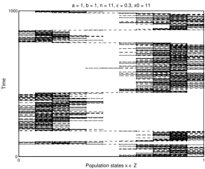
be the stochastic evolutionary game that results from the currency game under the BRM revision protocol with noise parameterε. Figure 1 gives an impres-sion of characteristic sample paths for a resulting evolutionary process with parameters a =b = 1, n= 11, ε= .3. It shows the characteristic punctuated equilibrium behavior, i.e., the sample path usually stays either near the popu-lation stateχ= 0 orχ= 1 for a long time while it switches infrequently to the other population state.
3
Markov State Models
Throughout what follows, let (Xk)k∈Nbe an irreducible, reversible discrete-time
Markov chain on a finite state spaceZ ={1,· · ·, l} with transition matrix P
and letµdenote its unique stationary distribution.
The basic idea of a Markov state models is to approximate the original Markov process by a Markov chain on a small finite state space. Thus, more
0 1000 0 1 Time Population states x ∈ Z a = 1, b = 1, n = 11, ε = 0.3, x0 = 11
Figure 1: Typical sample path of the number of players holding strategy 1 in the
evolutionary game defined by the currency game and the BRM revision protocol (a=b= 1,n= 11,ε=.3).
formally, our goal is to construct a Markov chain ( ˆXk)k∈N on the state space
ˆ
Z={1,· · · , m}withmconsiderably smaller thanlsuch that ( ˆXk) captures the
essential dynamics of the original Markov chain (Xk). In general, each of the
macrostates i ∈ Zˆ corresponds to a subset of states Ci ⊂ Z, called core sets,
where we assume that theCi’s are pairwise disjoint. Roughly speaking, the idea
is cluster the dynamics into core sets that may or may not partition the state space, but that represent the punctuated equilibrium dynamics in that
(i) the core sets carry most of the total statistical weight of the invariant distributionµof the original Markov chain and
(ii) the process resides inside each core set for a long time (relative to the typical time scale of the original chain).
In Section 3.1, we first consider the special case in which the core sets
C1,· · ·, Cm partition the state spaceZ, that is,
Ci∩Cj=∅fori6=j and m [
j=1
Cj=Z. (3.1)
Using this special case, we demonstrate formally the basic idea of the Markov state modeling approach. Subsequently, in Section 3.2, we explain how to gener-alize the special case. Finally, in Section 3.3, we discuss how to actually identify suitable core sets.
3.1
Full partition of state space and least-squares
approx-imation of Markov chains
In the special case in which these sets partition the state spaceZ, each macrostates
idirectly represents the subsetCiand we can define the reduced chain ( ˆXk) on
ˆ
Z={1,· · · , m}with transition matrix ˆP = (ˆpij) by
ˆ
pij =P[ ˜X1=j|X˜0=i], (3.2)
where ( ˜Xk)k∈Nis the discrete-time process on ˆZ that describes the dynamics of
(Xk) between the sets C1,· · ·, Cm, i.e.,
˜
Xk=i⇔Xk ∈Ci. (3.3)
Note that we have to differentiate between ( ˆXk) and ( ˜Xk) because ( ˜Xk) is
in general not Markovian.4 However, we still want to approximate (Xk) by a
Markov chain which is why we consider ( ˆXk).
Example. In our example of the currency game under BRM dynamics with parameters a = b = 1, n = 11, ε = .3, a reasonable partition of the set of population states into subsets such that there are only rare switches between them (see Figure 1) is A = {0,· · · ,5/11}, B = {6/11,· · · ,1}. The resulting matrix ˆP is given by (rounded to four digits)
ˆ P = .9989 .0011 .0011 .9989 . (3.4)
In order to appreciate the approximation properties of the reduced chain ( ˆXk) it is helpful to analyse the relation between the transition probabilities pij and ˆpij. To this end, suppose that the original chain starts in equilibrium, X0∼µ, withµ=PTµbeing the unique stationary distribution of (Xk). Now,
the transition probability ˆpij =Pµ[X1∈Cj |X0∈Ci] in (3.2) can be recast as
ˆ pij= P k,jpklχCi(l)χCj(k)µ(k) P kχCi(k)µ(k) , (3.5)
whereχC: Z → {0,1} denotes the indicator function of a setC ⊂Z, and the
notationPµ indicates thatX0is distributed according toµ.
Let us assume that the indicator functions χC1, . . . , χCm form a partition
of unity, i.e., P
iχCi(x) = 1, which is the case if the C1, . . . , Cm partition our
state space Z. The last equation can then be interpreted as the orthogonal projection onto the span of the functionsχC1, . . . , χCm with respect to the µ
-weighted scalar product
hf, giµ= X
k∈Z
f(k)g(k)µ(k) (3.6)
4The reason why ( ˜X
k) is not Markovian is called therecrossing problem. This name refers
to the issue that transitions between the subsets of state space are much more likely at the boundaries of the sets. This is, however, not such a big issue if the original process shows a strongly punctuated equilibrium dynamic behavior since the probability to be at the boundary is in this case negligible.
onRl. A compact way to write (3.5) thus is ˆ pij = hP χCi, χCjiµ hχCi, χCiiµ , (3.7)
which shows that the corresponding transition matrix ˆP = (ˆpij)i,j∈Zˆ is in fact
the orthogonal projection of P = (pij)i,j∈Z onto span{χC1, . . . , χCm},
under-stood as a linear subspace ofRl endowed with the weighted scalar productµ.
By being an orthogonal projection, ˆP is the best approximation ofP onto the space spanned by the indicator functions of the core setsC1, . . . , Cmin the
sense of least squares where the weighting with the invariant measureµarises naturally as a consequence of the fact that the Markov chain is initialized in its stationary distribution so as to make the macroscopic transition probabilities time-independent. Further notice that, since theχCi are non-negative and form
a partition of unity, the projected transition matrix ˆP is a stochastic matrix and inherits many important properties of the original transition matrixP:
1. IfP is irreducible and aperiodic, then so is ˆP.
2. ˆP has a unique invariant distribution ˆµ = (ˆµ(i))i∈Zˆ that equals the
marginal distribution of the core setsC1, . . . , Cm:
ˆ
µ(i) =hχCi, χCiiµ=µ(Ci), i∈Z.ˆ (3.8)
3. IfP is reversible with respect toµ, then ˆP is reversible with respect to ˆµ. A further advantage of (3.7) is that it tells us that, given a long realization of the original Markov chain (Xt) of lengthT, the expression
ˆ p(ijT)= PT t=1χCi(Xt)χCj(Xt+1) PT t=1(χCi(Xt)) 2 (3.9)
is an unbiased estimator of the macroscopic transition probabilities ˆpij. By the
assumption that µis unique and Z is finite, the law of large numbers implies that ˆp(ijT)converges almost surely to ˆpijasT → ∞for every initial valueX0= 0.
3.2
General core sets and sparse least-squares
approxima-tion
The case of a full partition of state space demonstrates the basic idea of Markov state models as a coarse-grained Markov chain that can be obtained by pro-jection onto suitable ansatz functions. In the general case, however, the sets
C1,· · ·, Cm do not necessarily partition the state space Z; thus, the approach
has to be modified since already the definition of the process ˜X in Eq. (3.3) is not well defined anymore.
In order to construct a reduced Markov chain that best approximates our original Markov chain in this case, the idea is to replace the set of indictator
functions by a clever “mollification”, forming a partition of unity and having support outside the setsC1, . . . , Cm. One such choice is the set of probabilistic
ansatz functions{q1, . . . , qm}, so-calledcommittor functions, defined by qi(x) =Pδx(τ
0
Ci < τ
0
C\Ci), (3.10)
where C = ∪iCi, δx is the point mass on x, and τAk = inf{k0 ≥ k|Xk0 ∈ A}
denotes the k-th hitting time for k ≥ 0. In words, the committor function
qi : Z → [0,1] is the function that gives for a state x ∈ Z the probability
that the Markov chain (Xk) will visit the set Ci first rather than C\Ci. By
construction, each qi is equal to one on Ci, equal to zero on the other sets Cj, j 6=i, and interpolates between these values outside the sets C1, . . . , Cm.
Moreover, since (Xt) is irreducible and positive recurrent (by Z being finite),
the process terminates after finite time with probability one by hitting one of the setsCi, independently of the initial conditionX0=x, and as a consequence
theqi sum up to one and form a partition of unity.
The analysis of the microscopic dynamics that is carried out in Sarich (2011) shows that the reduced Markov chain on ˆZcan be defined in terms of thequasi -transition matrix ˆP W−1, where the matrices ˆP andW are given by
ˆ P(i, j) = P(τCk+1 j < τ k+1 C\Cj | ˜ Xk=i), (3.11) W(i, j) = P(τCkj < τ k C\Cj | ˜ Xk =i), (3.12)
where ( ˜Xk) is themilestoning process defined by
˜
Xk=i⇔Xσ(k)=i, whereσ(k) = max{t≤k|Xt∈C}. (3.13)
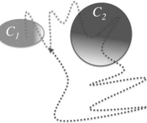
Equation (3.13) means that the milestoning process remains in statei as long as the original Markov chain (Xk) last visited core seti(see Figure 2). Thus, in
words,W(i, j) for j 6=igives the probability that the Markov chain next hits
Cj while being in a state inZ\Cat some timekand last came from core setCi,
whereC=∪m
j=1Cj. Similarly, ˆP(i, j) gives the probability that the next core set
hit isCj conditional on having hit the core setCilast at some timek. Moreover,
each macrostatei∈Zˆ is associated with the respective committor function qi
on the core set Ci and can thus be interpreted as representing the affiliation
with setCi. Note that while the definition of the quasi-transition matrix of our
Markov state model by ˆP W−1might not seem intuitively obvious, it reduces to
the matrix ˆP defined in Eq. (3.2) in the case of a full partition of state space. We call ˆP W−1a quasi-transition matrix since ˆP W−1is not always a
stochas-tic matrix (even thoughP andW are). We only know that its rows sum up to one since this is the case for both ˆP and W, and thus also forW−1 as well as
ˆ
P W−1. In the example given here as well as in the examples studied in Hallier
(2015) the entries of ˆP W−1are also non-negative, but in general the entries can
be negative as has been pointed out in Sarich (2011). It is possible to show, however, that ˆµdefined by
ˆ
µ(j) =X
i∈Z
Figure 2: Illustration of the milestoning process for two core setsC1andC2.
is the unique ergodic stationary distribution of ( ˆXk). Unlike in the case of a full
state space partition, the matrix ˆP W−1 does not trivially inherit all properties of the original chain, such as irreducibility, aperiodicity and reversibility; but ( ˆXk) is reversible with respect to ˆµif ˆP andW−1 commute.
Despite the apparent lack of structure preservation of the sparse core set approximation shows excellent spectral approximation properties, in that the dominant eigenvalues of the original chain are generally well approximated. The latter implies that the projected transition matrix can be used to accurately estimate transition rates between the core sets as well as mean residence times, and hence residence times and rates for the punctuated equilibria. Moreover, both matricesW and ˆP can be estimated from trajectory data in the following way: given a realization (x0,· · ·, xK) of (Xk) of lengthK, we can estimate
W∗,K(i, j) = ( RK ij rK i ifj6=i, 1−P j6=iW∗ ,K(i, j) otherwise, (3.15) ˆ P∗,K(i, j) = R +,K ij rK i , (3.16) whereRK
ij denotes the number of times where the chain came from core setCi,
is in a state in Z\C and hits Cj next, rKi is the total number of time steps
the trajectory was ini; that is, ˜Xk=i, andR
+,K
ij denotes the number of times
where the chain came from core setCi and hitCj next.
Example. Consider again the stochastic evolutionary game given in the last sec-tion. Let (Xt)t∈Tbe the birth-and-death chain with state spacez={0,
1
11,· · · ,1}.
We simulated the Markov chain witha= 1, b= 1, ε=.3, n= 11 to get a trajec-tory of population states (xt) fort= 1/11, . . . ,50000 and thus of length 5.5·105.
the estimated transition matrix ˆP∗W∗,−1 is given by ˆ P∗W∗,−1= .9993 .0007 .0007 .9993 . (3.17)
An analysis of the approximation error made (Hallier, 2015) shows that this is a better approximation of the underlying stochastic evolutionary game than the full partition Markov state model we considered above. In the example given, it shows that the approximation error is considerably smaller for the core set model, especially in the case of smaller population sizes and larger values of the noise parameterε. This is precisely the case where the other approximation approaches of stochastic evolutionary games cannot be applied. This example thus demonstrates that core set Markov state models fill a gap and constitute an important complement to existing approximation approaches.
Remark 3.1. Adopting a slightly more abstract point of the described clustering framework proves useful in deriving systematic error bounds for the Markov chain approximation. The idea is to view the clustering of the original Markov chain as a projection onto a linear subspace of the Hilbert space
H = ( f:Z →R : X k∈Z (f(k))2µ(k)<∞ ) (3.18)
of square summable functions endowed with the weighted scalar producth·,·iµ.
For example, in the first mentioned case, theµ-orthogonal projection of a func-tion f ∈ H onto span{χC1, . . . , χCm} can be understood as the best
approx-imation of f by functions that are measurable with respect to the partition {Ci: i = 1, . . . m}, measured in the natural norm on H that is induced by
h·,·iµ. In other words, the macroscopic transition probabilities ˆpij are the
con-ditional expectation, and hence least squares approximation, of the microscopic transition probabilitiespij, given only information about the macrostatesCi.
In the Markov state modelling approach due to Sch¨utte and co-workers (Deu-flhard and Weber, 2005; Huisinga and Schmidt, 2006; Sch¨utte and Sarich, 2013), the object of interest that is amenable to systematic approximations is the trans-fer operator, a family of linear operatorsPt:M+f → M
+
f that map any finite
non-negative Borel measure to a finite non-negative Borel measures. For our purposes, the transfer operator can be defined by
Ptν = PT t
ν , t∈N0, (3.19)
whereP is the transition matrix of the original Markov chain (Xt) and ν is a
counting density, understood as a non-negative column vector inRl. Note that
Pt preserves theL1 norm, i.e., if ν is a probability density, then so is Ptν for
allt. Given an initial distribution ofXt at t= 0, the transfer operator can be
transfers probability distributions in time and thus encodes information about the law of the process (Xt). Within the finite-state Markov chain framework
considered in this paper, approximating the transfer operator amounts to finding a suitable low-rank approximation of the transition matrixP.
Understanding the approximation of the original dynamics as a projection of the associated transfer operator, it is possible to show that the approximation error made with respect to the propagation of probability distributions as well as in terms of the dominant eigenvalues, which directly relate to the longest timescales of the original Markov chain, crucially depends on the projection error made; a small projection error implies a good approximation quality of our Markov state models (Hallier, 2015; Sarich, 2011).
3.3
Identification of core sets
While we outlined above how to construct Markov state models given core sets
C1,· · ·, Cm, the question remains of how to actually identify suitable core sets.
One approach is to use the results on the relationship between the approximation quality and the projection error. For full partition models, the projection error is as small as possible if the dominant right eigenvectors of the transfer matrix
P are as constant as possible on the sets of the partition. This relationship has been exploited by approaches that partition state space by clustering algorithms (as has, for example, been done in the molecular dynamics context by Krivov and Karplus, 2004; No´e et al., 2007; Rao and Caflisch, 2004). Similarly, in terms of core set Markov state models, finding core setsC1,· · ·, Cmso that the
projection error is as small as possible can be interpreted as a fuzzy clustering problem (Djurdjevac, 2012; Sarich, 2011).
In the case of stochastic evolutionary games with a noise parameter that determines the punctuated equilibrium behavior, we might also use the infor-mation given by its stationary distribution to identify possible core sets. More specifically, if the system under investigation depends on a noise parameter
ε > 0 in such a way that for smaller ε the punctuated equilibrium behavior increases, that is, for smallerεthe sample paths of the process stay even longer in certain subsets of the population state space and the switches between such subsets get more rare – just as in our example. In such a case, we can identify the setC =∪m
i=1Ci by comparing the stationary distributionµ∗ of the system
with noise levelε∗ with its propagated distribution Pθµ∗ = (PT)θµ∗ under a
decreased noise levelε < ε∗for a chosen timescaleθ >0 (see Remark 3.1). Note that thePtµ∗ ofµ∗ converges to the stationary distribution µ associated with
the stochastic evolutionary game at the lower noise levelε. Moreover, both sta-tionary distributionsµandµ∗ have the same form in the sense of local minima and maxima, but the stationary distributionµ∗ with increased noise intensity is less peaked. Now, the basic idea of the identification strategy is that a pop-ulation statexbelongs to the core set regionC if it gets more attractive in the stochastic evolutionary game with the decreased noise parameterε, i.e., if
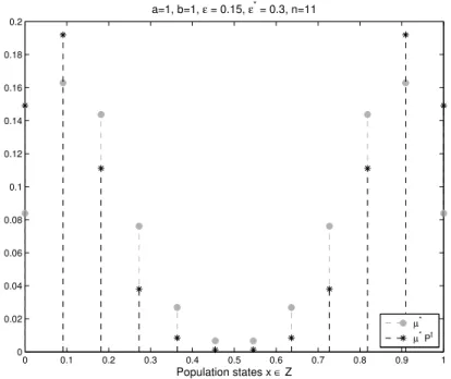
Example. In our example with parameters a = 1, b = 1, ε∗ = .3, ε = .15,
n= 11, this identification approach leads to the setC={0,1/11,10/11,1}for allθ∈T, which suggests the core setsC1={0,1/11}andC2={10/11,1}, see
also Figure 3.
As in this example, the clustering of C into core sets is usually straight-forward as the core sets are dynamically well separated. An advantage of the just sketched approach is that the necessary quantities can be estimated from trajectory data as well. Thus, it allows for a simulation-based approach to the construction of Markov state models. For more details, see Hallier (2015).
0 0.1 0.2 0.3 0.4 0.5 0.6 0.7 0.8 0.9 1 0 0.02 0.04 0.06 0.08 0.1 0.12 0.14 0.16 0.18 0.2 Population states x ∈ Z a=1, b=1, ε = 0.15, ε* = 0.3, n=11 µ* µ* Pt
Figure 3:Weights of the stationary distributionµ∗for the stochastic evolutionary
game of our running example with parametersa= 1, b= 1, ε∗ =.3, n= 11 and its propagationPt(µ∗) under the stochastic evolutionary game with parameters a= 1, b= 1, ε=.15, n= 11, t= 10/11.
4
Discussion and Outlook
We presented the Markov state modeling approach to extract the aggregated long term dynamics of stochastic evolutionary games. The approach is especially interesting for large, complex games in order to see the wood for the trees. In essence, Markov state models approximate the original Markov chain on a reduced state space. The transition probabilities between the macrostates can be estimated on the basis of short-term trajectory data. While this basic idea behind Markov state models has informally been used before (e.g., Kandori
et al., 1993), it is for the first time that the approach is formally considered and its approximation quality can be assessed.
Apparent advantages of a reduced state space are that it is easier to com-pute eigenvalues and eigenvectors as well as other properties such as waiting times. In addition, as our example demonstrates, the approximation of stochas-tic evolutionary games with punctuated equilibrium dynamics by Markov state models is especially interesting for small population sizes and larger mistake probabilities as traditional approximation techniques such as deterministic ap-proximation or stochastic stability analysis are not applicable or are of limited informative value.
One limitation is, however, that the approach and its analysis depends on the original Markov chain that captures the aggregated dynamics of the stochas-tic evolutionary game to be reversible. This is the case for the example we presented. More generally, stochastic evolutionary games that result from pop-ulation game with two strategies and full support revision protocols as well as those that result from finite-population games with clever agents under a logit choice revision protocol can be shown to have reversible dynamics (see Sandholm, 2010, Chapter 11.5.3, in addition, provides more general conditions on revision protocols under which finite-population potential games with clever agents result in reversible dynamics).
In general, it will be difficult to say whether it is reasonable to assume that a stochastic evolutionary game results in a reversible Markov chain. One reason for this difficulty is that, if we estimate the transition matrix from simulated trajectory data, it does not need to fulfill the detailed balance equation, even if the underlying Markov chain is reversible (No´e, 2008; Prinz et al., 2011). In the context of molecular dynamics, however, it was possible to derive approxima-tive models that can be proven to be reversible although the original model is not. An example is the diffusion model, which represents an approximation to the Langevin model in the limit of high friction (see, e.g., Sch¨utte and Sarich, 2013, Chapter 2 and references therein). As a future research question, it seems worthwhile to explore whether similar results can be obtained for stochastic evo-lutionary games; that is, whether there are approximations of certain stochastic evolutionary games that can be shown to be reversible.
Beyond that, we would like an approach that applies also to non-reversible Markov dynamics. Notice that it is not difficult to derive a construction of a matrix representation of the core set Markov state models for given core sets in the case of non-reversible Markov chains (see, e.g., Djurdjevac, 2012; Djurdjevac et al., 2010). However, we neither have results with respect to their approximation quality nor an approach to the identification of core sets for non-reversible Markov chains. One fundamental problem is that the eigenvalues and eigenvectors of the transfer matrices corresponding to non-reversible Markov chains need not be real anymore. In this case, the interpretation of the spectral information is unclear. Up to now, there are few approaches that apply also to non-reversible Markov chains (Eckhoff, 2002; Gaudilli`ere and Landim, 2011; Horenko, 2011; Sarich and Sch¨utte, 2014). A graph-theoretical framework for constructing reversible surrogates of non-reversible dynamics, based on a cycle
decomposition of the underlying Markov chain, has been suggested in Banisch (2015), however the applicability to evolutionary games is yet open.
The identification of Markov state models for general stochastic evolutionary games is therefore an open problem and will be a topic of future research.
References
Banisch, R. (2015).Markov Processes Beyond Equilibrium and Optimal Control. PhD thesis, Fachbereich Mathematikund Informatik, FU Berlin.
Benaim, M. and Weibull, J. (2003). Deterministic approximation of stochastic evolution in games. Econometrica, 71:873–903.
Bovier, A. (2009). Metastability. In Koteck´y, R., editor, Methods of Contem-porary Mathematical Statistical Physics, Lecture Notes in Mathematics 1970. Springer-Verlag Berlin Heidelberg.
Deuflhard, P. and Weber, M. (2005). Robust perron cluster analysis in confor-mation dynamics. Linear Algebra and its Applications, 398:161184.
Djurdjevac, N. (2012). Methods for analyzing complex networks using random walker approaches. PhD thesis, Fachbereich Mathematikund Informatik, FU Berlin.
Djurdjevac, N., Sarich, M., and Sch¨utte, C. (2010). On Markov state models for metastable processes. In Proceedings of the International Congress of Mathematicians, Hyderabad, India.
Eckhoff, M. (2002). The low lying spectrum of irreversible, infinite state Markov chains in the metastable regime. Preprint.
Ellison, G. (2000). Basins of attraction, long-run stochastic stability, and the speed of step-by-step evolution. The Review of Economic Studies, 67(1):17– 45.
Foster, D. and Young, P. (1990). Stochastic evolutionary game dynamics. The-oretical Population Biology, 38:219–232.
Gaudilli`ere, A. and Landim, C. (2011). A Dirichlet principle for non reversible Markov chains and some recurrence theorems.Probability Theory and Related Fields, 158:55–89.
Hallier, M. (2015). Formalization and Metastability Analysis of Agent-Based Evolutionary Models. PhD thesis, Fachbereich Mathematikund Informatik, FU Berlin.
Hofbauer, J. and Sigmund, K. (2003). Evolutionary game dynamics. Bulletin (New Series) of the American Mathematical Society, 40(4):479–519.
Horenko, I. (2011). Parameter identification in nonstationary Markov chains with external impact and its application to computational sociology. SIAM Multiscale Modeling & Simulation, 9(4):1700–1726.
Huisinga, W. and Schmidt, B. (2006). Metastability and dominant eigenvalues of transfer operators. In Leimkuhler, B., Chipot, C., Elber, R., Laaksonen, A., Mark, A., Schlick, T., Sch¨utte, C., and Skeel, R., editors,New Algorithms for Macromolecular Simulation, volume 49 ofLecture Notes in Computational Science and Engineering, pages 167–182. Springer.
Jaeger, C. (2008). Mathematics and the social sciences: The challenge ahead. Introductory contribution to the Dahlem Conference: ”Is There a Mathe-matics of Social Entities”?, December 2008, Berlin, Germany. Unpublished manuscript.
Jaeger, C. C. (2012). Scarcity and coordination in the global commons. In Jaeger, C. C., Hasselmann, K., Leipold, G., Mangalagiu, D., and T´abara, J. D., editors, Reframing the Problem of Climate Change: From Zero Sum Game to Win-Win Solutions, pages 85–101. Routledge.
Kandori, M., Mailath, G. J., and Rob, R. (1993). Learning, mutation, and long run equilibria in games. Econometrica, 61(1):29–56.
Krivov, S. V. and Karplus, M. (2004). Hidden complexity of free energy surfaces for peptide (protein) folding.Proceedings of the National Academy of Sciences of the United States of America, 101:1476614770.
Kurtz, T. (1970). Solutions of ordinary differential equations as limits of pure jump Markov processes. Journal of Applied Probability, 7:49–58.
No´e, F. (2008). Probability distributions of molecular observables computed from Markov models. The Journal of Chemical Physics, 128:244103.
No´e, F., Horenko, I., Sch¨utte, C., and Smith, J. C. (2007). Hierarchical anal-ysis of conformational dynamics in biomolecules: Transition networks of metastable states. The Journal of Chemical Physics, 125:155102.
Prinz, J.-H., Wu, H., Sarich, M., Keller, B., Senne, M., Held, M., Chodera, J. D., Sch¨utte, C., and No´e, F. (2011). Markov models of molecular kinetics: Generation and validation. The Journal of Chemical Physics, 134(174105). Rao, F. and Caflisch, A. (2004). The protein folding network. Journal of
Molecular Biology, 342(1):299306.
Sandholm, W. H. (2010). Population Games and Evolutionary Dynamics. MIT Press, Cambridge.
Sandholm, W. H. (2011). Stochastic evolutionary game dynamics: foundations, deterministic approximation, and equilibrium selection. Sigmund, Karl (ed.), Evolutionary game dynamics. American Mathematical Society short course,
January 4–5, 2011, New Orleans, Lousiana, USA. Providence, RI: American Mathematical Society (AMS). Proceedings of Symposia in Applied Mathe-matics 69, 111-141 (2011).
Sarich, M. (2011).Projected Transfer Operators. PhD thesis, Fachbereich Math-ematikund Informatik, FU Berlin.
Sarich, M. and Sch¨utte, C. (2014). Utilizing hitting times for finding metastable sets in non-reversible Markov chains. Technical Report 14-32, Konrad-Zuse-Zentrum f¨ur Informationstechnik Berlin.
Sch¨utte, C. and Sarich, M. (2013). Metastability and Markov State Models in Molecular Dynamics: Modeling, Analysis, Algorithmic Approaches, volume 24 ofCourant Lecture Notes. American Mathematical Society.
Weibull, J. W. (1995). Evolutionary Game Dynamics. MIT Press, Cambridge. Young, H. P. (1993). The evolution of conventions. Econometrica, 61(1):57–84. Young, H. P. (1998). Individual Strategy and Social Structure. Princeton
Uni-versity Press.
Young, H. P. (2006). Social dynamics: Theory and applications. In Tesfatsion, L. and Judd, K. L., editors,Handbook of Computational Economics: Agent-Based Computational Economics, volume 2, chapter 22, pages 1081–1108. North-Holland.