Original citation:
Gironacci, Elia, Mousavi Nezhad, Mohaddeseh, Rezania, Mohammad and Lancioni, Giovanni. (2017) A non-local probabilistic method for modeling of crack propagation. International Journal of Mechanical Sciences
Permanent WRAP URL:
http://wrap.warwick.ac.uk/96298
Copyright and reuse:
The Warwick Research Archive Portal (WRAP) makes this work by researchers of the University of Warwick available open access under the following conditions. Copyright © and all moral rights to the version of the paper presented here belong to the individual author(s) and/or other copyright owners. To the extent reasonable and practicable the material made available in WRAP has been checked for eligibility before being made available.
Copies of full items can be used for personal research or study, educational, or not-for-profit purposes without prior permission or charge. Provided that the authors, title and full
bibliographic details are credited, a hyperlink and/or URL is given for the original metadata page and the content is not changed in any way.
Publisher’s statement:
© 2017. This manuscript version is made available under the CC-BY-NC-ND 4.0 license
http://creativecommons.org/licenses/by-nc-nd/4.0/
A note on versions:
The version presented here may differ from the published version or, version of record, if you wish to cite this item you are advised to consult the publisher’s version. Please see the ‘permanent WRAP URL’ above for details on accessing the published version and note that access may require a subscription.
A non-local probabilistic method for modelling of crack propagation
1Elia Gironacci1, Mohaddeseh Mousavi Nezhad1, Mohammad Rezania1, Giovanni Lancioni2 2
3
1Computational Mechanics, Civil Research Group, School of Engineering, University of Warwick, 4
Coventry, CV4 7AL, UK
5
2Department of Civil Engineering and Architecture (DICEA), Polytechnic University of Marche 6
(UNIVPM), Via Brecce Bianche, 60131, Ancona, Italy
7
8
9
ABSTRACT 10
Damage process in engineering systems is strongly affected by spatial heterogeneity and local 11
discontinuities in the materials, which are significantly influencing the reliability and integrity 12
of the systems. In this paper, we present a new stochastic approach as a tool for performing 13
uncertainty quantification in simulating damage evolution in heterogeneous brittle materials. 14
One of the advantages of the proposed method is its ability to capture the influence of 15
uncertainty in the mechanical properties of whole simulation domain, not just the properties of 16
the immediate neighbourhood around the crack tip, on direction of crack propagation. In fact, 17
through this approach the direction of crack propagation at a specified point of localised 18
damage can be probabilistically determined based on nonlocal mechanics theory, in which the 19
influence of local discontinuities and weak points located at further distances from the crack 20
tip, in addition to those located at the immediate neighbourhood of the local damage, are 21
incorporated into the model. The reliability and performance of the methodology are examined 22
through simulation of numerical examples and comparison with analytical results and 23
experimental data. The case studies show how the crack initiation angle can be reasonably 24
estimated with this methodology and how this approach provides realistic values of fracture 25
toughness KIC and fracture energy Gf.
26
Key Words: stochastic crack initiation angle; fracture toughness; mixed-mode fracture; nonlocal approach;
non-27
Gaussian random field 28
1. Introduction 33
In recent years, many researchers have focused on the problem of modelling heterogeneous 34
material systems containing discontinuities. Numerous methodologies for inclusion of 35
heterogeneity in numerical frameworks for simulating material failure behaviour have been 36
developed, which can be grouped into two main categories: multi-scale models and stochastic 37
approaches. 38
Multi-scale methods have offered a significant progress in explicitly describing local 39
heterogeneities [1]. In fact, for the heterogeneous materials, like concrete, rocks or composites, 40
often a local fine-scale definition of micro-structure of the materials that influence their 41
macroscopic mechanical response is needed [2]. Developed understanding of multiple phase 42
concepts is used in multi-scale techniques, where it is aimed to predict the joint multi-phase 43
response of structures. Although multi-scale modelling has been proved to be a powerful 44
method for incorporation of the heterogeneity, difficulties may arise when a detailed 45
knowledge of the material micro-structure for identifying the representative elementary 46
volume, is not available. For this reason, an increasing interest has now been directed towards 47
stochastic approaches, as they allow probabilistic estimation of degree of heterogeneity in the 48
materials by quantifying fluctuations of mechanical properties [3-6, 46]. 49
50
The two main processes for brittle failure of materials are crack initiation and crack 51
propagation. From a physical point of view, when a body is deformed, the corresponding stored 52
strain energy increases. If there is a high enough imbalance in the energy of the system is high 53
enough, fracturing occurs due to progressive degradation of material strength. The failure 54
process can be therefore broken down into a number of steps based on the level of material 55
degradation and stiffness softening. [7]. Within these steps, crack initiation denotes the stress 56
level in which micro-fracturing is occurring [8]. Crack growth happens at the instance of 57
critical energy release and lasts until when the micro-cracks have joined and the structure can 58
no longer support an increase in the load. 59
60
One of the elements appreciably influenced by the material heterogeneity, is the crack initiation 61
angle, in particular for those systems that are subjected to mixed-mode loading conditions [9-62
11]. In a recent work, Lin and his co-workers [12] proved, with experimental measurements on 63
acoustic emissions of mortar materials, that the crack angle is correlated with the magnitude of 64
recognised by Park and Lange [13], in which a new fracture parameter, named critical crack 66
opening angle, describing the crack opening resistance, has been introduced for cement-based 67
materials. Yang et al. [14] studied the effect of loading type and heterogeneity on the crack 68
geometry, initiation and propagation processes, and concluded that local stresses control crack 69
initiation process, while the loading configuration is responsible for crack inclination and 70
curving. Evangelatos and Spanos [15] used the peridynamic theory to study the effect of the 71
inclination of crack initiation angle on the total energy of a system, estimation of its reliability 72
and its probability of failure. 73
Another crucial material property, influencing crack initiation and propagation process, is 74
fracture toughness, which represents the critical stress intensity factor (SIF) at crack tip, that 75
can introduce catastrophic crack growth. Fracture toughness is a function of applied loading, 76
crack size and structural geometry, and it is representative of the level of “stress” at the tip of 77
the crack [11]. A high value of fracture toughness makes materials resistant to catastrophic 78
crack extension; alternatively, it may be considered as requiring a large amount of strain energy 79
to create new surfaces. 80
An accurate and rigorous evaluation of fracture toughness is therefore indispensable for 81
application of fracture mechanics methods in structural integrity assessment. The American 82
Society for Testing and Materials (ASTM) provides standard terminology and formulations 83
with regards to experimental measurements of fracture toughness [16-17]. In parallel with the 84
experimental methods, closed form solutions for analytical calculation of fracture toughness, 85
for determined geometries and loading configurations, have also been developed, and they are 86
expressed as linear combination of SIFs for different crack opening modes [18-24]. 87
If for a given problem that has to be examined, no experimental measurement of fracture 88
toughness is conducted, often values for fracture toughness are chosen from the literature. 89
However, not necessarily a specific value can be used for specific case studies, as fracture 90
toughness depends not only on the constituents of the material, but also on other factors such 91
as geometrical configurations and loading conditions. This assumption may therefore lead to 92
erroneous results and, possibly, to an overestimation of the material resistance. 93
One of the analytical criteria, which is most frequently used for investigating mixed mode 94
fracture toughness, is the maximum tangential stress (MTS) criterion, where fracture toughness 95
is explicitly expressed as a function of mode I and II SIFs and of the crack initiation angle. 96
Several studies (e.g. [25-26]) revealed that this method, which considers the tangential stresses 97
in the vicinity of the crack tip, especially in the case of mixed mode fracture may not provide 98
detailed study on this matter, reporting experimental values of fracture toughness of four 100
different types of rock materials and comparing them with the analytical results from the MTS 101
method; they showed that if the effect of a non-singular stress term, called T-stress, is 102
considered, then a better agreement between analytical and experimental results can be 103
achieved. This modified criterion, called generalised maximum tangential stress (GMTS) 104
method, has been applied for several specimens subjected to mixed-mode loading, but none of 105
them includes the effect of material heterogeneity in the calculation of the fracture toughness. 106
The aim of this study is therefore to extend and implement the definition of the GMTS criterion 107
for materials with heterogeneous structure. 108
The computational framework used in this study for extracting a probabilistic distribution of 109
the crack initiation angle, employs a phase-field formulation [27], in which the initiation and 110
evolution of crack are described by a scalar damage variable assuming values in the range (0,1), 111
where 1 means sound material, and 0 means totally broken material. The non-local analysis of 112
the damage field evolution in an area in proximity of the crack initiation point allows to 113
determine in which direction crack is most likely to propagate. Crack propagation direction is 114
predicted using a probabilistic approach which includes a linear combination of different 115
Probability Density Functions (PDF) of crack initiation angle. 116
Finally, in the context of stochastic modelling, energy release rate is defined as a function of 117
the randomly variable fracture toughness and a probabilistic distribution of the damage 118
initiation in the fracturing body is sought. Therefore, the damage state in proximity of the crack 119
initiation point is considered to define realistic values of fracture toughness, which is a function 120
of initial crack angle, loading condition and geometry. A probabilistic distribution for crack 121
propagation direction is then defined and used for sampling the angle and calculating fracture 122
toughness for the heterogeneous materials. 123
The main advantage of the method proposed in this work is the possibility to simply and 124
practically quantify the uncertainty in the fracture toughness value evaluation as a function of 125
other mechanical properties of the material which are directly introduced in a phase-field theory 126
based framework for crack propagation. The material length scale, representative of the size of 127
the damage zone, contributes in defining the degree of heterogeneity of the material. In this 128
way, the statistical information (mean value, standard deviation and correlation length) needed 129
for sampling random values for crack initiation angle will be automatically provided by the 130
numerical simulations using the phase-field theory. Furthermore, it will be proved that the non-131
Gaussian nature of the fracture toughness and fracture energy can be automatically captured 132
any translation function for sampling random values of these material properties [4-5]. 134
135
2. Fracture advancement methodology and damage state of the body 136
In this section, the basic ingredients of the phase-field model used to determine the initiation 137
and propagation of fracture are presented. The variational model proposed in [27-28] is 138
considered, where smeared fracture in an elastic body is described by means of a scalar 139
damage field s, which assumes values in the range (0, 1); when s = 1 the material is sound, and, 140
when s = 0, it is totally damaged. The internal energy assigned to is 141
142
𝐸(𝐮, 𝑠) = ∫ {𝑘12 tr−(∇𝐮)2+ 𝑠2[𝑘1
2 tr+(∇𝐮)2+ 𝜇 (∇𝐮𝟐− 2
3tr(∇𝐮)2)]} 𝑑𝑥
𝛺
+𝐺𝑓
2 ∫ (𝜀∇𝑠𝟐+
(1 − 𝑠)𝟐
𝜀 ) 𝑑𝑥
𝛺
(1)
143
which depends on the displacement field u and on the damage s. The first integral in Eq. (1) 144
represents the bulk energy, where 𝑘 = 𝜆 + 2𝜇/3 is the bulk modulus, and are the Lame’s 145
coefficients, and the decomposition tr+(∇𝐮) = max{tr(∇𝐮), 0} and tr−(∇𝐮) = {tr(∇𝐮), 0} in 146
positive and negative parts of the trace of ∇𝐮 is used. The second integral is the fracture energy, 147
which is the sum of a local and a non-local contributions. Gf is the unit fracture energy, and
148
is an internal length associated to damage non-locality. The length is related to the size of the 149
process zone, as discussed in the following. The energy (1) is minimised under the 150
irreversibility condition 𝑠̇ ≤ 0, introduced to forbid material self-healing. 151
By using the energy (1), different fracture processes are reproduced when tensile or 152
compressive loadings are applied. Indeed, in regions of subjected to tensile states, where 153
volume changes are positive, the opening and evolution of brittle fractures are allowed; while, 154
in compressed regions, where volume changes are negative, cracks are partially forbidden, and 155
only shear fractures can develop, when shear stresses are generated by compressive loadings. 156
When a fracture forms, the damage parameter s assumes the value s = 0 on the fracture surface, 157
and it increases by moving away from that surface. The optimal profile of s in the direction 158
normal to the fracture surface was determined in [29], and its expression is 159
𝑠(𝑥) = 1 − e−|𝑥−𝑥0|𝜀 , (2)
161
where x is the coordinate in the direction normal to the surface, and x0 is the intersection point
162
between the normal axis and the surface. From Eq. (2), at distances larger than 2.5 from the 163
surface (|x-x0| > 2.5), damage attains values s > 0.9, and the material can be considered
164
practically sound. Thus the damaged band around the fracture surface has a thickness of about 165
5, which represents the size of the process zone. 166
The functional (1) is numerically minimised by using the incremental procedure first proposed 167
in [30], and described in the following. We denote with t the loading parameter of the problem 168
(load or displacement applied on a portion of the body boundary), which is monotonically 169
increased from 0 by means of finite increments. At each loading step, an iterative procedure is 170
performed. Let (ui1,si1) be the solution at the (i-1)th loading step, the pair (ui,si) at the ith step
171
is evaluated by solving the iterative double minimisation procedure shown below. 172
1. Initiation. Set (ui0, si0)=(ui-1,si-1)
173
2. Iteration j. For given (ui j-1, si j-1)
174
i. compute ui j by minimizing (, si j-1)
175
ii. compute si j by minimizing (ui j , )
176
iii. Irreversibility condition: set si j(x)=min{ si j(x) , si-1(x)}, x
177
3. Iterate step 2 until | si j - si j-1|L∞<smax, with smax being a fixed tolerance.
178
At the step i = 0 it is set that (u0,s0) = (0,1), so the body is assumed undeformed and uncracked
179
in the initial configuration. 180
The minimizations at steps i. and ii. are performed by finding the stationarity point of (1), 181
keeping s and u fixed, respectively. The corresponding problems are linear elliptic and 182
solutions are numerically found by means of the finite element method. Within the Matlab 183
environment, an in-house code is developed based on triangular elements with affine shape 184
functions. To improve the accuracy in the determination of the field s, the program includes a 185
mesh refinement algorithm, which automatically subdivides those elements at which the values 186
of s become smaller than a given threshold. As a result, within each loading step, in the 187
algorithm an iterative macro-scheme, which includes the process described above, allows for 188
the mesh refinement. While the convergence of the developed algorithm has not been proven 189
In the next sections, two dimensional simulations are performed by assuming the hypothesis 191
of plane strain state. 192
193
3. Fracture toughness calculation: the GMTS criterion 194
In the context of linear elastic fracture mechanics, elastic stresses in proximity of the crack tip 195
can be written as linear combinatio of angular functions expanded according to infinite series 196
[25]. Based on the GMTS criterion, for a brittle material, crack propagates radially and 197
perpendicular to the direction of maximum tangential stress; the crack initiation point is where 198
the tangential stress 𝜎𝜃𝜃 reaches its critical value, and along this direction crack initiates at rc
199
defined as the critical distance from the crack tip. It is considered that rc is a constant material
200
property; it is usually considered to be equal to the radius of the process zone. Several methods, 201
both experimental and numerical, have been proposed to estimate the size of this zone for brittle 202
materials [25, 31]. In this work, rc is considered to be compatible with the size of the process
203
zone estimated on the basis of the theory discussed in the Section 2, therefore, equal to 204
5Formulation of the tangential stress in the vicinity of crack tip is therefore explicitly given 205
as series expansion in [25] as 206
207
𝜎𝜃𝜃= 1 √2𝜋𝑟cos
𝜃
2[𝐾𝐼cos2 𝜃 2−
3
2𝐾𝐼𝐼sin 𝜃] + 𝑇 sin2𝜃 + 𝑂(√𝑟) (3)
208
where r and 𝜃 are the polar coordinates of a point with respect to the crack tip, KI and KII are
209
the SIFs for mode I and II respectively and T is the T-stress, which is a constant term defining 210
the stress parallel to the crack and independent of r, the higher order term 𝑂(√𝑟) of the 211
expansion can be neglected in proximity of the crack tip. 212
Recalling that crack initiates and propagates in the direction of maximum tangential stress, the 213
crack initiation angle 𝜃0 (angle that indicates the direction with respect to the direction of the 214
initial notch, where the maximum stresses are found) can be calculated by imposing the 215
condition 216
217
𝜕𝜎𝜃𝜃
𝜕𝜃 |𝜃=𝜃0 = 0. (4)
218
The calculated angle is used for obtaining the value of the fracture toughness of mixed-mode 219
provides the following expression [25] 221
222
√2𝜋𝑟𝑐 𝜎𝜃𝜃𝑐 = cos
𝜃0
2 [𝐾𝐼cos2 𝜃0
2 − 3
2𝐾𝐼𝐼sin 𝜃0] + 𝑇 sin2𝜃0. (5) 223
If now the pure mode-I fracture case is considered, 𝐾𝐼𝐼, 𝑇 and 𝜃0 all become equal to zero. 224
Therefore, when fracture occurs 𝐾𝐼 reaches its critical value 𝐾𝐼𝑐 which corresponds to the
225
mode-I fracture toughness 226
227
√2𝜋𝑟𝑐 𝜎𝜃𝜃𝑐 = 𝐾𝐼𝑐. (6)
228
Eq. (5) can be rewritten using Eq. (6) to obtain the value for fracture toughness 𝐾𝐼𝑐
229
230
𝐾𝐼𝑐 = cos𝜃0
2 [𝐾𝐼cos2 𝜃0
2 − 3
2𝐾𝐼𝐼sin 𝜃0] + 𝑇 sin2𝜃0. (7) 231
The expression in Eq. (7) represents the final form of the GMTS criterion. Closed form 232
solutions for 𝐾𝐼, 𝐾𝐼𝐼 and 𝑇 have been calculated for defined geometries and loading 233
configurations [25-26, 32-37]. 234
General expression for 𝐾𝐼 and 𝐾𝐼𝐼 takes the general form 235
236
𝐾𝐼= 𝜎∗√𝜋𝑎 𝐹 𝐼(
𝑎
𝑊) (8)
𝐾𝐼𝐼 = 𝜎∗√𝜋𝑎 𝐹 𝐼𝐼(
𝑎
𝑊), (9)
237
where 𝜎∗ represents the stress field in correspondence of the crack tip, a provides information 238
about the position and the length of the crack, W is a measure of the body geometry, 𝐹𝐼(𝑊𝑎) 239
and 𝐹𝐼𝐼(𝑊𝑎) are dimensionless functions of the geometry of the notched body and of the 240
experimental setup. For calculating the values for 𝑇, one of the most common methods is based 241
on its calculation from finite element analysis as shown by Ayatollahi et al. [26]. 242
243
4. Uncertainty quantification: the spectral representation method 244
In this work, uncertainty is included in the model by sampling random values of 𝜃0 using the
spectral representation method. With this method, a stochastic field of a two dimensional 246
problem is expressed as [5] 247
𝜃𝑔(𝑖)(𝑥, 𝑦) =𝜃0+√2 ∑ ∑ [𝐴𝑛1𝑛2 (1) cos (𝜅
1𝑛1𝑥 + 𝜅2𝑛2𝑦 + 𝜙𝑛1𝑛2 (1)(𝑖)) 𝑁2−1
𝑛2=0 𝑁1−1
𝑛1=0
+ 𝐴𝑛(2)1𝑛2cos(𝜅1𝑛1𝑥 − 𝜅2𝑛2𝑦 + 𝜙𝑛(2)(𝑖)1𝑛2)]
(10)
248
where 𝜙𝑛(1)(𝑖)1𝑛2 and 𝜙𝑛(2)(𝑖)1𝑛2 are the realisation for the ith simulation of the independent random
249
phase angles which follow a uniform distribution. Furthermore, 250
𝐴𝑛(1)1𝑛2= √2𝑆𝑔𝑔(𝜅1𝑛1, 𝜅2𝑛2)∆𝜅1∆𝜅2 (11a)
𝐴𝑛(2)1𝑛2= √2𝑆𝑔𝑔(𝜅1𝑛1, −𝜅2𝑛2)∆𝜅1∆𝜅2 (11b)
251
𝜅1𝑛1= 𝑛1𝛥𝜅1 (12a)
𝜅2𝑛2 = 𝑛2𝛥𝜅2 (12b)
252
𝛥𝜅1 = 𝜅1𝑢/𝑁1 (13a)
𝛥𝜅2 = 𝜅2𝑢/𝑁2 (13b)
253
with 254
𝑛1= 0, 1, … , 𝑁1− 1; 𝑛2= 0, 1, … , 𝑁2− 1. (14)
255
𝑁1 and 𝑁2 are the number of intervals where the wave number axes are split, 𝜅1𝑢 and 𝜅2𝑢 are
256
defined as the upper cut-off wave numbers defining the active region of the spectral density 257
function (SDF) 𝑆𝑔𝑔. Therefore, the effect of 𝑆𝑔𝑔 is operative only for the range 258
259
−𝜅1𝑢≤ 𝜅1 ≤ 𝜅1𝑢 and −𝜅2𝑢≤ 𝜅2 ≤ 𝜅2𝑢; (15)
260
outside of this range, 𝑆𝑔𝑔 is assumed to be equal to 0. 261
263
𝑆𝑔𝑔= 𝜎𝑔2 𝑏1𝑏2 4𝜋 exp [−
1 4(𝑏1
2𝜅
12+ 𝑏22𝜅22)] (16)
264
where 𝜎𝑔 is the standard deviation of the field, while 𝑏1 and 𝑏2 represent the correlation length
265
along the two dimensions. 266
267
5. PDF of the crack initiation angle 𝛉𝟎 268
The uncertainty in the material behaviour is related to heterogeneity of the materials strength 269
that is modelled by defining a random distribution of damage inside of simulation domain. 270
Therefore, similar to the work presented by Gutierrez and de Borst [45], damage parameter 271
instead of material stiffness or fracture energy has been selected as a random parameter. 272
However, due to lack of experimental data and information about the statistics of damage 273
distribution throughout of the material, a computational model has been used to generate a 274
hypothetical possible spatially random field for damage parameters associated to materials with 275
different micro-structure and length scales. The random distribution of damage parameter is 276
linked with the material length scale and particle size distribution (as an index of material 277
heterogeneity) through specifying several threshold values for 𝑠̅. This aspect also overcomes 278
the issue of the mesh dependency, as the size of the mesh is directly connected to the material 279
length scale as shown in Section 6 in the definition of the parameters for Eq. (1). Different 280
threshold values for damage parameter 𝑠̅ have been selected in a way to take into account both 281
the influence of distribution of imperfection in the whole specimen and the possible variations 282
in the size of the specimens. Without this, the approach would not be non-local, as it would 283
consider only the damage in proximity of the crack tip. 284
285
Therefore, for a given body discretised in finite elements and for a given crack initiation point, 286
positions of the finite element nodes with respect to the crack tip and associated values of s are 287
considered. In order to accurately take into account the contribution of the damage state of the 288
body in the definition of θ0, the so-called fracture process zone (FPZ) should be adequately
289
identified. The FPZ can be identified numerically with the phase-field theory described above. 290
In fact, the damage will spread from the crack tip at a distance which will be included within 291
The values for damage in each node provide information about the direction that the crack is 293
most likely to initiate and propagate: in particular, it is likely that the crack spreads through 294
those nodes with a lower value of damage. Therefore, the degree of damage that develops in 295
the body is considered in the procedure formed by the following steps: 296
1. Calculate the values for damage parameter by using the iterative procedure described 297
in Section 2; 298
2. For different threshold values 𝑠̅, select the nodes with 𝑠 ≤ 𝑠̅; 299
3. Calculate the polar coordinates with respect to the crack tip of the nodes selected in step 300
2; 301
4. Estimate mean value of 𝜃0 for each threshold value 𝑠̅; 302
5. Calculate the overall mean value and the standard deviation of 𝜃0 from the values 303
estimated in step 4 for each 𝑠̅; 304
6. Sample values of 𝜃0 using the spectral method described in Section 4 and calculate the 305
corresponding values of KIc using Eq. (7).
306
Through this method, 𝜃0 becomes the parameter with stochastic nature and can be then 307
expressed as a vector 𝜽0𝑔 = [𝜃𝑔(1), 𝜃𝑔(2), … , 𝜃𝑔(𝑛𝐹𝐸)], with 𝑛𝐹𝐸 being the number of elements 308
forming the finite element mesh that discretises the problem under investigation. Therefore, 309
the probabilistic generalised maximum tangential stress (PGMTS) criterion can be achieved in 310
terms of 𝜃0𝑔 using Eq. (7) as
311
312
𝑲𝑰𝒄(𝜽0𝑔 ) = cos
𝜽0𝑔
2 [𝐾𝐼cos2 𝜽0𝑔
2 − 3
2𝐾𝐼𝐼sin 𝜽0𝑔 ] + 𝑇 sin2𝜽0𝑔 . (17) 313
Finally, fracture energy Gf can also be calculated using the elastic crack-tip solution and a
314
simple relationship between KIc and Gf as [40]:
315
𝐾𝐼𝑐2
𝐸′ = 𝐺𝑓, (18)
which is developed based on the theories of Griffith [7]. In the Eq. 18, 𝐸′ = 𝐸 for the plane 316
stress conditions, and 𝐸′= 𝐸/(1 − 𝜈2) for the plane strain conditions with 𝐸 being Young’s 317
modulus and 𝜈 Poisson’s ratio. 318
319
6.1. Notched concrete slab 321
In order to verify the proposed methodology, the first example considered in this study is a 322
finite element model of a concrete slab with size of 500 mm x 400 mm (see Fig. 1). This 323
example was also simulated by Huang et al. [41]. Young’s modulus E and Poisson’s ratio 𝜈 are 324
chosen equal to 25000 N/mm2 and 0.18 respectively. An initial deterministic value for Gf equal
325
to 0.15 N/mm is assigned to the model [3]. A value of mm is selected, while the size of 326
the mesh is chosen to be equal to 8 mm. The value for is chosen, following the considerations 327
listed in [29], on the basis of the average size of the material constituents; in particular, is 328
typically assumed to be 2-3 times the characteristic material length scale. As concrete is formed 329
by constituents of different sizes, an average dimension of 4-5 mm is here considered and, 330
consequently, the value of 8 mm for is selected. An initial crack of dimension 4 x 40 mm is 331
modelled in the middle of the specimen. In order to create a typical mixed mode crack 332
condition, the inclination of the crack with respect to the distributed load is set to be 45º. The 333
simulation is performed in quasi-static displacement-controlled condition. 334
In order to calculate KIc using Eq. (7), the value of rc has been selected according to the
335
recommendations proposed in [25 and 38-39]. In [25] rc is calculated for the brittle materials
336
as a function of KIc and a range of values between 45 and 60 N/mm3/2 was assumed for KIc,
337
which gives a range of values between 35 and 45 mm for rc, approximately. In [38] and [39] a
338
combination of analytical and experimental investigations on concrete specimens subjected to 339
both pure mode-I and mixed-mode loading provided a range of values for the size of FPZ, 340
which vary from a minimum of 40 up to a maximum of 140 mm. Therefore, the value of rc for
341
this example is chosen equal to 40 mm which is within the range proposed in the literature. 342
For this specific example, the explicit formulation of Eq. (8) and (9) are expressed, together 343
with the explicit expression for 𝑇, as [32] 344
345
𝐾𝐼= 𝜎√𝜋𝑎 sin2𝛽 (19a)
𝐾𝐼𝐼 = 𝜎√𝜋𝑎 sin 𝛽 cos 𝛽 (19b)
𝑇 = 𝜎 cos 2𝛽 (19c)
346
where, 𝜎 is applied stress to the body, a is half length of the initial notch, and 𝛽 is inclination 347
angle of the notch with respect to the loading direction. For this example 𝜎= 8.6 N/mm2, a = 348
Fig. 2 shows the evolution of the damage in proximity of the crack tip that has been taken into 350
account to generate PDFs of 𝜃0. For simplicity, only the upper half of the specimen is 351
considered and presented in Fig. 2. The area where the damage spreads, is smaller than the size 352
of FPZ considered in literature [38-39], which vary from a minimum of 40 mm up to a 353
maximum of 140 mm for pure mode I failure. 354
Table 1 summarizes the values obtained for crack initiation angle with respect to the direction 355
of the notch, considering different values of 𝑠̅ together with the calculated mean value and 356
standard deviation. In order to validate the result, the mean value is compared with the results 357
from literature [41] and with the value calculated considering the condition [25] 358
359
[𝐾𝐼sin 𝜃0+ 𝐾𝐼𝐼(3cos 𝜃0− 1)] −
16
3 𝑇√2𝜋𝑟𝑐cos 𝜃0sin 𝜃0
2 = 0 (20)
360
which is the explicit form of Eq. (4). For this example, Huang et al. [41] provided a value for 361
crack initiation angle equal to 53.1º, while the result obtained using Eq. (20) is 52.7º. The 362
summary of all the results can be found in Table 1. It can be observed that the value reported 363
in [41] and the value calculated through the methodology proposed in this work differ about 364
4º. 365
The mean value and standard deviation shown in Table 1 are then considered as an estimate to 366
sample random values for 𝜃0 using the Gaussian process shown in Eq. (10). 367
In the first instance, a deterministic value of the fracture toughness is calculated using Eq. (7) 368
and the mean value of 𝜃0. The fracture toughness is therefore equal to 60.9 N/mm3/2. Griffith’s 369
Energy Gf is then calculated as Gf = 0.14 N/mm, consistent with the range of values of Gf for
370
concrete found in literature [3, 42]. 371
This example is one of those used in literature to study mixed-mode conditions for the 372
materials. For this reason, this example has been used with the main purpose of comparing the 373
crack initiation angle available in literature with the value crack initiation angle as mean value 374
of the probabilistic distribution obtained. 375
With regards to the parameters involved in the stochastic approach described in section 4, the 376
number of terms used for the spectral representation series is chosen as N1 = N2 = 20, the
cut-377
off wave numbers 𝜅1𝑢= 𝜅2𝑢 = 2𝜋 and b1 = b2 = 1 [30]. Once the mean value and standard
378
deviation for 𝜃0 are defined, they are used to sample values of 𝜃0 according to a Gaussian
379
distribution, as shown in Fig. 3. This sample for 𝜃0 is then substituted into the expression for 380
KIcof Eq. (7), and a sample for KIc is then obtained as shown in Fig. 4. The sample shown has
a mean value of 60.5 N/mm3/2. The calculated values of KIc can finally be used to get a
382
distribution, shown in Fig. 5, of the values for Gf with mean value 0.14 N/mm and standard
383
deviation of approximately 5%. It is worth noting, as shown in the Figs. 4 and 5, that the values 384
of KIc and Gf don’t follow the same Gaussian trend of 𝜃0, but a non-Gaussian trend. In
385
particular, the probability functions plotted in the Figs. 4 and 5 follow a Weibull distribution. 386
This trend is consistent with the conclusion from several works [3, 5] that heterogeneous 387
distributions of Gf follow a non-Gaussian (either lognormal or Weibull) distributions. This
388
results show that the proposed methodology is capable to automatically capture the non-389
Gaussian distribution of a given normally-distributed statistical information (e.g. mean value, 390
standard deviation, correlations), using the translation field functions, which satisfy specific 391
constrains and compatibility conditions associated to the related random field [5]. In fact, 392
despite the simplicity of the Gaussian distributions for sampling from simple statistical 393
information, their use for creating a sample of fracture toughness may lead to the generation of 394
negative, and therefore physically meaningless, values. With the method proposed in this work, 395
we will be able to benefit from the simplicity of Gaussian field theory while generating a 396
realistic and physically meaningful distribution for KIC.
397
398
6.2 The four-point Single-Edge Notched Shear (SENS) beam 399
The second example used in this study is the four-point SENS beam studied in [43]. This 400
benchmark is one of the most widely used to validate numerical models for simulating mixed-401
mode crack propagation in concrete. A wide range of experimental data is available in 402
literature, and a satisfactory crack scatter is available and has been summed up in [44]. 403
Specimen geometry, boundary conditions and material properties about this benchmark are 404
shown in Fig. 6. Young’s modulus E is equal to 24800 N/mm2, and Poisson’s ratio is equal to 405
0.18. Because also for this second case study a concrete specimen is considered, a value for 406
mm is again selected, while the size of the mesh is chosen equal to 5 mm. For the same 407
reason, the values for the parameters involved in the definition of the spectral representation 408
method are chosen as in the previous case study. 409
For this benchmark, the explicit form of Eq. (8) and (9) for 𝐾𝐼 and 𝐾𝐼𝐼 take the form [18] 410
411
𝐾𝐼=
𝐹 𝐵𝑊(1 −
𝑑
𝐿) 𝐹𝐼√𝜋𝑎 (21a)
𝐾𝐼𝐼 = 𝐹 𝐵𝑊(1 −
𝑑
𝐿) 𝐹𝐼𝐼√𝜋𝑎
412
where F is the force applied to the specimen, and is selected equal to 132.2 kN, B is the 413
specimen thickness equal to 152 mm, W is the specimen height equal to 306 mm, d = 61 mm 414
is the distance from the middle of the specimen of the force applied and the pin , L is half of 415
the total length of the specimen equal to 458 mm and a is the length of the initial notch equal 416
to 82 mm. FI and FII are geometry functions depending on specimen geometry and their values
417
for these two functions are available in [18]. Value for T is equal to -0.04 N/mm2, calculated 418
in [35] from Finite Elements analysis. As discussed by Smith et al. [32], T can have negative 419
values. 420
For this example, from Eq. (21a) and (21b), FI = -0.1 and FII = 1.12. Mode-I and Mode-II SIFs
421
can be hence calculated and they are equal to -3.9 N/mm3/2 and 44.5 N/mm3/2. It is worth 422
noticing that Mode-I SIF has also a negative value. This happens when (i) shear-mode is 423
prevalent on opening-mode mechanisms and (ii) crack lips closure prevails over crack opening 424
[35]; therefore, physically this means that mode-I opening mode has a very small influence of 425
the fracturing process. With this regards, Fig. 7 shows the variation of FI over the variation of
426
the ratio d/W (as d/W increases, the shear failure prevails over opening failure). It can be seen 427
that when d/W decreases, shear effect increases, making the value for FI smaller, until it
428
disappears for d/W > 1.5. 429
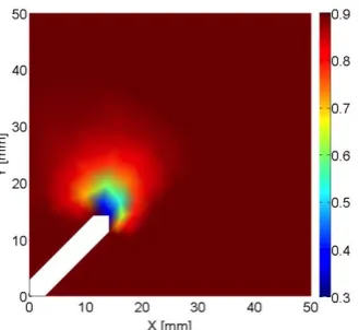
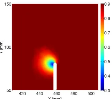
Fig. 8 shows the evolution of damage in proximity of the initial notch, and it is considered for 430
the generation of the mean value and standard deviation of 𝜃0. As can be seen, also for this
431
case study the area where the damage spreads is compatible with the size of FPZ considered in 432
literature [25, 38-39]. 433
Table 2 summarizes the values of crack initiation angle with respect to the direction of the 434
initial notch, obtained considering different values of 𝑠̅ together with the calculated mean value 435
and standard deviation. 436
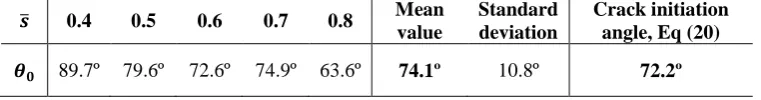
The obtained mean value of 𝜃0 is equal to 74.1º with respect to the direction of the initial notch. 437
The value of 𝜃0 calculated using Eq. (20) is equal to 72.2º, which is in good agreement with 438
the value obtained numerically. As for the previous example, the deterministic values of 439
fracture toughness and fracture energy are first calculated: KIc is equal to 48.1 N/mm3/2 while
440
Griffith’s Energy Gf is then calculated as Gf = 0.095 N/mm.
441
Once the mean value and standard deviation for 𝜃0 are defined as listed in Table 2, different
442
values of crack initiation angle are sampled using the spectral approach, as shown in Figure 9. 443
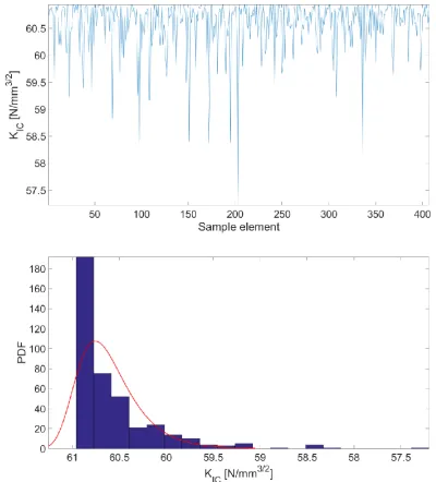
This sample is then used together with the expression for KIc(i.e., Eq. (7)), and a sample for
444
KIc is then obtained as shown in Fig. 10. The sample has a mean value of 48.22 N/mm3/2. The
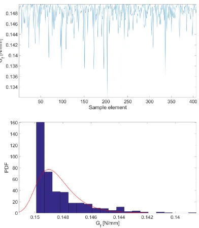
calculated values of KIc is finally used to get a distribution of the values for Gf which have
446
mean value of 0.094 N/mm and standard deviation of approximately 4%. It is worth noting, as 447
shown in Figs. 10 and 11, that also for this example KIc and Gf follow a log-normal trend,
448
consistent with the conclusion from the previous example and from literature [3,5] that 449
heterogeneous distributions of KIc and Gf follow a non-Gaussian trend.
450
451
7. Conclusions 452
A novel approach for uncertainty quantification of the random fields in the physical domains 453
is presented. The uncertainty in the mechanical properties of the bodies subjected to damage is 454
quantified by considering the damage state developed in the vicinity of the crack initiation 455
points. Distribution of the damage, predicted using a phase-field model capable of reproducing 456
mixed mode loading conditions, is then employed to estimate the mean value and the standard 457
deviation for direction of crack evolution in the body. This statistical information is then used 458
to create samples for the crack initiation angle by means of the Gaussian spectral representation 459
approach. The calculated sample is finally used to calculate spatially-varying values of the 460
fracture toughness, and consequently the fracture energy for the mixed-mode crack propagation 461
conditions. In first instance, a concrete slab with an internal notch with an inclination of 45º 462
and subjected to uniaxial traction is studied. Calculated mean value for the crack initiation 463
angle (57.1º), is in a good agreement with value of the crack initiation angle found in literature 464
(53.1º), with a difference of only 4º. The second example studied is the four-point bending 465
beam, one of the examples most widely used to validate models considering the mixed-mode 466
conditions. Also for this case study, the mean value for the crack initiation direction (74.1º with 467
respect to the direction of the initial notch) is in very good agreement with the value calculated 468
analytically (72.2º). For both examples, the calculated values of the fracture toughness and the 469
fracture energy are in excellent agreement with values from literature. Furthermore, the most 470
interesting aspect of this method is its capability, by using Gaussian-related statistical 471
information, to capture the non-Gaussian nature of the statistical distribution of the fracture 472
toughness and fracture energy for brittle materials. 473
474
Acknowledgement 475
This study was supported by EPSRC UK (No. EP/M506679/1). 476
477
References
[1] Geers MG, Kouznetsova VG, Brekelmans WA. Multi-scale computational homogenization: trends and 479
challenges. J Comput Appl Math 234(7), 2010, 2175-2182. 480
[2] Miehe C, Bayreuther CG. On multiscale FE analyses of heterogeneous structures: from homogenization to 481
multigrid solvers. Int J Numer Methods Eng 71(10), 2007, 1135-1180.
482
[3] Yang Z, Xu XF. A heterogeneous cohesive model for quasi-brittle materials considering spatially varying 483
random fracture properties. Comput Method Appl M 197(45), 2008, 4027-4039. 484
[4] Stefanou G. The stochastic finite element method: past, present and future. Comput M Appl M. 198(9), 485
2009, 1031-1051. 486
[5] Georgioudakis M, Stefanou G, Papadrakakis M. Stochastic failure analysis of structures with softening
487
materials. Eng Struct 61, 2014, 13-21.
488
[6] Yang ZJ, Su XT, Chen JF, Liu GH. Monte Carlo simulation of complex cohesive fracture in random
489
heterogeneous quasi-brittle materials. Int J Solids Struct 46(17), 2009, 3222-3234.
490
[7] Griffith AA. The phenomena of rupture and flow in solids. Philos T Roy Soc A 221, 1921, 163-198. 491
[8] Eberhardt E, Stead D, Stimpson B, Read RS. Identifying crack initiation and propagation thresholds in brittle 492
rock. Can Geotech J 35(2), 1998, 222-233. 493
[9] Kim JH, Paulino GH. T-stress, mixed-mode stress intensity factors, and crack initiation angles in 494
functionally graded materials: a unified approach using the interaction integral method. Comput Method 495
Appl Mech 192(11), 2003, 1463-1494. 496
[10]Li YP, Chen LZ, Wang YH. Experimental research on pre-cracked marble under compression. Int J Solids 497
Struct 42(9), 2005, 2505-2516. 498
[11]Aliha MR, Ayatollahi MR, Smith DJ, Pavier MJ. Geometry and size effects on fracture trajectory in a 499
limestone rock under mixed mode loading. Eng Fract Mech 77(11), 2010, 2200-2212. 500
[12]Lin C, Zhu W, Li S, Guo Y, Wen N, Yang L. Influence of 3D-crack angle on strength of mortar
501
material. Yantu Lixue/Rock Soil Mech 27(SUPPL.), 2006, 622-626.
502
[13]Park CW, Lange DA. Fracture Parameters and Post-Peak Behavior Evaluation under LEFM on Bonded 503
Cement-Based Materials. InKey Engineering Materials. Vol. 324, 2006, 587-590). Trans Tech Publications. 504
[14]Yang YF, Tang CA, Xia KW. Study on crack curving and branching mechanism in quasi-brittle materials 505
under dynamic biaxial loading. Int J Fract 177(1), 2012, 53-72. 506
[15]Evangelatos GI, Spanos PD. A collocation approach for spatial discretization of stochastic peridynamic 507
modeling of fracture. J Mech Mater Struct 6(7), 2011, 1171-1195. 508
[16]ASTM E1823-10a. Standard terminology relating to fatigue and fracture testing, 2011, American Society
509
for Testing and Materials.
510
[17]ASTM E1820-11. Standard test method for measurement of fracture toughness, 2011, American Society for
511
Testing and Materials.
512
[18]Fett T. Stress intensity factors and weight functions for special crack problems Vol. 6025, 1998, FZKA. 513
[19]Chang SH, Lee CI, Jeon S. Measurement of rock fracture toughness under modes I and II and mixed-mode
514
conditions by using disc-type specimens. Eng Geol 66(1), 2002, 79-97.
515
[20]Aliha MRM, Ayatollahi MR, Kharazi B. Numerical and Experimental Investigations of Mixed Mode
516
Fracture in Granite Using Four-Point-Bend Specimen. Damage Fract Mech 2009,275-283.
517
[21]He, MY, Hutchinson JW. Asymmetric four-point crack specimen. J Appl Mech 67(1), 2000, 207-209.
518
[22]Shahani AR, Tabatabaei SA. Computation of mixed mode stress intensity factors in a four-point bend
519
specimen. Appl Math Model 32(7), 2008, 1281-1288.
520
[23]Lim IL, Johnston IW, Choi SK, Boland JN. Fracture testing of a soft rock with semi-circular specimens
521
under three-point bending. Part 1—mode I. Int J Rock Mech Min 1994, 185-197.
522
[24]Lim IL, Johnston IW, Choi SK, Boland JN. Fracture testing of a soft rock with semi-circular specimens
523
under three-point bending. Part 2—mixed-mode. Int J Rock Mech Min 1994, 199-212.
524
[25]Ayatollahi MR, Aliha MR. On the use of Brazilian disc specimen for calculating mixed mode I–II fracture
525
toughness of rock materials. Eng Fract Mech 75(16), 2008, 4631-4641
[26]Ayatollahi MR, Pavier MJ, Smith DJ. Determination of T-stress from finite element analysis for mode I and
527
mixed mode I/II loading. Int J Fract 91(3), 1998, 283-298.
528
[27]Amor H, Marigo JJ, Maurini C. Regularized formulation of the variational brittle fracture with unilateral 529
contact: numerical experiments. J Mech Phys Solids 57(8), 2009, 1209-1229. 530
[28] Freddi F, Royer-Carfagni G, Regularized variational theories of fracture: a unified approach. J Mech Phys 531
Solids 58, 2010, 1154–1174. 532
[29]Lancioni G, Royer-Carfagni G. The variational approach to fracture mechanics. A practical application to
533
the French Panthéon in Paris. J Elast 95(1-2), 2009, 1-30.
534
[30]Bourdin B, Francfort GA, Marigo JJ. Numerical experiment in revisited brittle fracture. J Mech Phys Solids
535
48, 2000, 797-826.
536
[31]Schmidt RA. A microcrack model and its significance to hydraulic fracturing and fracture toughness 537
testing. The 21st US Symposium on Rock Mechanics (USRMS), 1980, American Rock Mechanics 538
Association. 539
[32]Smith DJ, Ayatollahi MR, Pavier MJ. The role of T‐stress in brittle fracture for linear elastic materials under
540
mixed‐mode loading. Fatigue Fract Eng M 24(2), 2001, 137-150.
541
[33]Fett T. Stress Intensity Factors, T-stresses, Weight Functions: Supplement Volume, 2009, KIT Scientific
542
Publishing.
543
[34]Ayatollahi MR, Aliha MRM. Wide range data for crack tip parameters in two disc-type specimens under
544
mixed mode loading. Comp Mater Sci 38(4), 2007, 660-670.
545
[35]Ayatollahi MR, Aliha MRM. On the use of an anti‐symmetric four‐point bend specimen for mode II
546
fracture experiments. Fatigue Fract Eng M. 2011,34.11:898-907.
547
[36]Ayatollahi MR, Aliha MRM. Fracture toughness study for a brittle rock subjected to mixed mode I/II
548
loading. Int J Rock Mech Min 44(4), 2007, 617-624.
549
[37]Ayatollahi MR, Aliha MRM. Mixed mode fracture analysis of polycrystalline graphite–a modified MTS
550
criterion. Carbon 46(10), 2008, 1302-1308.
551
[38]Dong W, Wu Z, Zhou X, Dong L, Kastiukas G. FPZ evolution of mixed mode fracture in concrete: 552
experimental and numerical. Eng Fail Anal 75, 2017, 54-70. 553
[39] Yao W, Wu KR, Li ZJ. Fracture process zone of composite materials as concrete. Third International 554
Conference on Fracture Mechanics of Concrete and Concrete Structures(FRAMCOS-3). 1998. 555
[40]Irwin GR. Analysis of stresses and strains near the end of a crack traversing a plate. Spie Milestone Ser MS 556
137(167-170), 1997, 16. 557
[41]Huang D, Lu G, Liu Y. Nonlocal Peridynamic Modeling and Simulation on Crack Propagation in Concrete 558
Structures. Math Probl Eng 2015, 2015. 559
[42]Fernández-Canteli A, Castañón L, Nieto B, Lozano M. Determining fracture energy parameters of concrete
560
from the modified compact tension test. Frattura ed Integrità Strutturale 30, 2014, 383.
561
[43]Arrea M. Mixed-mode crack propagation in mortar and concrete, 1982, Cornell University. 562
[44]Most T. Stochastic crack growth simulation in reinforced concrete structures by means of coupled finite 563
element and meshless methods. 2005. 564
[45]Gutierrez M. and de Borst, R. Deterministic and stochastic analysis of size effects and damage evolution in
565
quasi-brittle materials. Arch Appl Mech 69, 1999, 655-676.
566
[46]Mousavi Nezhad M, Gironacci E, Rezania M, Khalili N. (2017) Stochastic modelling of crack propagation
567
in materials with random properties using isometric mapping for dimensionality reduction of nonlinear data
568
sets.Int J Numer Methods Eng (In Press), 2017.
577 578 579 580 581 582 583 584 585 586 587 588 589 590 591 592 593 594 595
596
597
598
599
600
601
Figures
602
603
Fig 1. Geometry and loading condition of the considered concrete panel with an inclined central notch.
606
Fig 2. Local area in proximity of the crack tip for the notched concrete panel: the effect of the damage
607
influences the direction of crack initiation considering the damage state at the time step immediately before
608
failure starts.
609 610
611
[image:21.595.219.384.72.223.2]Fig 3. Sample for 350 values of 𝜃0 (top) and PDF with Gaussian nature (bottom). The method shown in Eq. (10) 613
is used to generate each sample.
614
615
616
Fig 4. Sample of KIc generated from the sample of crack initiation angle (top) and relative PDF (bottom): it can
617
be observed that the PDF follows a non-Gaussian distribution, result consistent with assumptions from literature
[image:22.595.86.487.108.551.2]618
[3-5].
619 620
621
623
624
Fig 5. Sample of Gf calculated from KIc (top) and relative Probabilistic distribution of one sample of Gf: it can
625
be observed that its behaviour follows a lognormal distribution, behaviour consistent with the assumption that
626
non-Gaussian distributions well describe the physical trend of brittle materials such as concrete. [3-5].
[image:23.595.93.486.81.531.2]629
Fig 6. Geometry and load of the SENS beam.
630 631
632
Fig 7. Geometric function FI trend as function of d/W for L/W = 3.0 and a/W = 0.3. FI has negative values for
633
small values of d/W, and increases its values for increasing d/W. For larger values (d/W > 1.5) the contribution
634
of mode I component vanishes.
635 636
637
Fig 8. Local area in proximity of the crack tip of the four point SENS beam: the effect of the damage influences
638
also for this example the direction of crack initiation. Nodes closed to the crack tip have a lower value of
639
damage and therefore a higher influence for the determination of the crack initiation angle.
[image:24.595.154.423.74.254.2] [image:24.595.116.469.315.508.2] [image:24.595.208.388.570.729.2]641
642
643
Fig 9. Sample for 2300 values of 𝜃0 (top) and PDF with Gaussian nature (bottom). The method shown in Eq. 644
(10) is used to generate each sample.
[image:25.595.98.485.95.533.2]648
[image:26.595.95.489.83.524.2]649
Fig 10. Sample of KIc generated from the sample of crack initiation angle (top) and relative PDF (bottom): the
650
PDF follows also in this case a non-Gaussian distribution [3-5].
654
[image:27.595.93.485.82.521.2]655
Fig 11. Sample of Gf calculated from KIc (top) and relative Probabilistic distribution of one sample of Gf: Also
656
in this example its behaviour follows a Gaussian trend, behaviour consistent with the assumption that
non-657
Gaussian distributions well describe the physical trend of brittle materials such as concrete. [3-5].
658 659 660
661
662
663
664
665
666
667
Tables
669
Table 1. Mean values for 𝜃0 estimated in proximity of the crack tip for different threshold values of 𝑠̅
670
𝒔̅ 0.4 0.5 0.6 0.7 0.8 Mean
value 𝜽𝟎
Standard deviation
Crack initiation angle, [41]
Crack initiation angle, Eq (20)
𝜽𝟎 45º 65.3º 60.3º 56.9º 58º 57.1º 7.5º 53.1º 52.7º
671
[image:28.595.109.490.234.284.2]672
Table 2. Values for 𝜃0 estimated in proximity of the crack tip for different threshold values of 𝑠̅ 673
𝒔̅ 0.4 0.5 0.6 0.7 0.8 Mean
value
Standard deviation
Crack initiation angle, Eq (20)
𝜽𝟎 89.7º 79.6º 72.6º 74.9º 63.6º 74.1º 10.8º 72.2º

![Fig 10. Sample of KIc generated from the sample of crack initiation angle (top) and relative PDF (bottom): the PDF follows also in this case a non-Gaussian distribution [3-5]](https://thumb-us.123doks.com/thumbv2/123dok_us/9429204.448058/26.595.95.489.83.524/sample-generated-sample-initiation-relative-follows-gaussian-distribution.webp)