Advance Access publication 2016 February 23
Submillimeter array observations of NGC 2264-C: molecular outflows
and driving sources
Nichol Cunningham,
1,2‹Stuart L. Lumsden,
1Claudia J. Cyganowski,
3,4Luke T. Maud
1,5and Cormac Purcell
61School of Physics and Astronomy, University of Leeds, Leeds LS2 9JT, UK
2National Radio Astronomy Observatory, PO Box 2, Green Bank, WV 24944, USA
3Scottish Universities Physics Alliance (SUPA), School of Physics and Astronomy, University of St Andrews, St Andrews, Fife KY16 9SS, UK
4Harvard–Smithsonian Center for Astrophysics, Cambridge, MA 02138, USA
5Leiden Observatory, Leiden University, PO Box 9513, NL-2300 RA Leiden, the Netherlands
6Sydney Institute for Astronomy, University of Sydney, NSW 2006, Australia
Accepted 2016 February 12. Received 2016 February 11; in original form 2014 October 17
A B S T R A C T
We present 1.3 mm Submillimeter Array (SMA) observations at∼3 arcsec resolution towards
the brightest section of the intermediate/massive star-forming cluster NGC 2264-C. The mil-limetre continuum emission reveals ten 1.3 mm continuum peaks, of which four are new detections. The observed frequency range includes the known molecular jet/outflow tracer
SiO (5−4), thus providing the first high-resolution observations of SiO towards NGC 2264-C.
We also detect molecular lines of 12 additional species towards this region, including CH3CN,
CH3OH, SO, H2CO, DCN, HC3N, and12CO. The SiO (5−4) emission reveals the presence of
two collimated, high-velocity (up to 30 km s−1with respect to the systemic velocity) bipolar
outflows in NGC 2264-C. In addition, the outflows are traced by emission from12CO, SO,
H2CO, and CH3OH. We find an evolutionary spread between cores residing in the same parent
cloud. The two unambiguous outflows are driven by the brightest mm continuum cores, which are IR-dark, molecular line weak, and likely the youngest cores in the region. Furthermore,
towards the Red MSX Source AFGL 989-IRS1, the IR-bright and most evolved source in
NGC 2264-C, we observe no molecular outflow emission. A molecular line rich ridge feature, with no obvious directly associated continuum source, lies on the edge of a low-density cavity and may be formed from a wind driven by AFGL 989-IRS1. In addition, 229 GHz class I maser emission is detected towards this feature.
Key words: stars: formation – ISM: jets and outflows – ISM: molecules.
1 I N T R O D U C T I O N
Can high-mass star formation be described as a scaled-up version of low-mass star formation? Protostellar jets and outflows are a ubiquitous feature of the star formation process; as such, their study provides an important means of addressing this fundamental ques-tion. Observationally, young stellar objects (YSOs) of all masses are known to drive bipolar molecular outflows. If a single driving mechanism operates in both the low- and high-mass regimes (e.g.
Richer et al.2000), this would be evidence for a common
forma-tion process. The initial evidence for a single mechanism was an observed correlation, over five orders of magnitude, between bolo-metric luminosity and outflow force, power and mass flow rate (e.g.
Cabrit & Bertout1992; Shepherd & Churchwell1996). Outflows
E-mail:[email protected]
observed towards massive young stellar objects (MYSOs) can con-tain momentum, mass and energy up to a few orders of magnitude
larger (e.g. Beuther et al.2002; Wu et al.2004; Zhang et al.2005)
than outflows observed towards lower mass YSOs (e.g. Kim &
Kurtz2006).
A single outflow mechanism would imply that all stars acquire mass by a similar disc-accretion process that scales with source luminosity. However, outflows observed towards MYSOs were ini-tially suggested to be less collimated than those identified towards
low-mass YSOs (e.g. Wu et al.2004). In contrast, both Beuther
et al. (2004) and Zhang et al. (2005) identified similar degrees of
collimation towards the jets/outflows driven by young MYSOs as found in jets/outflows from low-mass YSOs. To account for both low and high degrees of collimation of massive outflows, Beuther
& Shepherd (2005) proposed a scenario in which an initially
well-collimated jet/outflow de-collimates with time, eventually forming a wide angle wind. In the early formation stages outflows driven
2016 The Authors
at University of St Andrews on April 11, 2016
http://mnras.oxfordjournals.org/
Figure 1. HerschelPACS 70μm emission (grey-scale, the emission is plotted on a log scale) overlaid with contours of SCUBA 450μm emission (dashed green) and N2H+(1−0) integrated intensity (PdBI, magenta). The N2H+(1−0) integrated intensity map was presented in Peretto et al. (2007) and provided to us by N. Peretto, the contours are the same as given in that paper and are from 1 Jy beam−1to 5 Jy beam−1in steps of 1 Jy beam−1. The SCUBA contours are given by 1σ=0.9 Jy beam−1×5,10,20,30,40,50,60. Blue crosses (x) mark the positions of millimetre sources reported by Peretto et al. (2006,2007); yellow stars mark the positions of the brightest 24μmSpitzerpoint sources in the region (taken directly from the archive mosaic). The section of NGC 2264-C presented in this work is shown by the dashed black circle which represents the 10 per cent power level of the SMA primary beam centred on RA (J2000) 06h41m10.s13, Dec. (J2000) 09◦2934.0.
by MYSOs are potentially magnetically dominated and therefore
highly collimated (e.g. HH80/81; Carrasco-Gonz´alez et al.2010).
For more evolved MYSOs, a radiatively driven stellar wind
natu-rally gives rise to a less collimated outflow (e.g. Vaidya et al.2011).
Intermediate-mass YSOs (2 M ≤M∗≤8 M) link the
low-and high-mass regimes, low-and so have the potential to provide key insights into whether outflow properties scale smoothly with the mass of the driving (proto)star. A complication is that intermedi-ate and high-mass stars generally form in clustered environments
(Lada & Lada2003); as a result, it is not always unambiguously
clear from observations which core(s) in a region are powering the jet/outflow(s), particularly at lower spatial resolution. High angular resolution studies that can resolve individual cores and outflows are thus crucial to understanding jets/outflows from intermediate and high-mass stars.
We targeted NGC 2264-C, one of the nearest
intermediate/high-mass star-forming regions in the RedMSXSource (RMS) survey
(Lumsden et al.2013), with the Submillimeter Array (SMA). The
aim of these observations was to resolve the SiO emission seen with the James Clerk Maxwell Telescope (JCMT, Section 2.2), and so
identify which source(s) in the region are drivingactiveoutflows.
A particular goal was to assess the relationship of the RMS source to the outflows seen at low angular resolution, and so to aid in the interpretation of a large, low-resolution outflow survey of RMS
objects (Maud et al.2015).
Located in the Mon OB1 giant molecular cloud complex at a
distance of 738+−5750 pc (Kamezaki et al. 2014), NGC-2264-C is
a comparatively well-studied region, with a wealth of ancillary
data and known CO outflows. AFGL 989-IRS1 (Allen 1972), a
9.5 MB2 star, dominates the region in the IR. 13 millimetre
con-tinuum sources have been identified (Ward-Thompson et al.2000;
Peretto, Andr´e & Belloche 2006; Peretto, Hennebelle & Andr´e
2007, see Fig.1), which have typical diameters of∼0.04 pc and
masses ranging from∼2 to 40 M (Peretto et al.2006, 2007).
From comparing observations and SPH simulations, Peretto et al.
(2007) suggest that NGC 2264-C is in a global state of collapse on
to the central, most massive millimetre core, C-MM3 (∼40 M).
Maury, Andr´e & Li (2009) observed12CO (2−1) emission with the
IRAM 30 m (∼11 arcsec resolution), detecting a network of 11
out-flow lobes with projected velocities ranging from 10 to 30 km s−1,
lengths of 0.2–0.8 pc and momentum fluxes in the range 0.5–
50×10−5M
km s−1yr−1. However, the limited angular
resolu-tion meant that only a small minority of the detected outflow lobes could be unambiguously identified with driving sources (millimetre continuum cores). Subsequent high-resolution SMA observations
by Saruwatari et al. (2011) focusing on the central class 0
protostel-lar core, C-MM3, identified a compact, young north–south bipoprotostel-lar
outflow driven by this source in both12CO and CH
3OH emission,
emphasizing the power of high-resolution, multiline observations. The ambiguity in identifying outflow driving sources based on low-resolution single-dish observations calls for high angular reso-lution observations of a reliable jet/outflow tracer. Silicon monoxide (SiO) emission is an effective tracer of jets/outflows from both
low-mass YSOs (e.g. Gibb et al.2004; Sakai et al.2010; Tafalla et al.
2010; L´opez-Sepulcre et al.2011; Codella et al.2014) and MYSOs
(e.g. Gibb, Davis & Moore2007; Codella et al.2013; Leurini et al.
at University of St Andrews on April 11, 2016
http://mnras.oxfordjournals.org/
2013; S´anchez-Monge et al.2013). Importantly, SiO emission, un-like CO, does not suffer from confusion with easily excited ambient material. CO emission can also be easily excited in outflows, which may obscure the underlying effects; it is possible for weak outflows to effectively be ‘fossil’ momentum-driven remnants even after the
central driving engine declines (e.g. Klaassen et al.2006; Hunter
et al.2008). In contrast, SiO requires the passage of fast shocks
to release it into the gas phase (e.g. Gusdorf et al.2008a; Guillet,
Jones & Pineau Des Forˆets2009) and thus is an excellent tracer
of the fast shocks associated with an active outflow near the stellar
driving source (e.g. Schilke et al.1997).
We present the first high angular resolution study (∼3 arcsec
resolution with the SMA) of SiO (5−4) emission towards NGC
2264-C. The main goals of the SMA observations are to identify activeoutflows and their central driving sources, and to determine the relationship of these active outflows to the multiple outflows previously reported based on single-dish observations of the region. In Section 2, we summarize the observations presented in this paper. We present our results in Section 3, discuss the physical properties of the detected cores and outflows in Section 4, and summarize our conclusions in Section 5.
2 O B S E RVAT I O N S A N D DATA R E D U C T I O N
2.1 SMA observations
Our SMA1observations were made with eight antennas in the
com-pact configuration on 2010 December 12. The pointing centre for the
observations is RA (J2000) 06h41m10s.13, Dec. (J2000) 09◦2934.0.
We observed on-source for a total of∼4 h, spread over an 8 h track
to improve UV coverage. The system temperatures ranged from
∼100 to 180 K depending on source elevation. A typical value
of τ(225 GHz)∼0.1–0.15 was obtained during the observations. At
1.3 mm, the SMA primary beam is∼55 arcsec (FWHP), and the
largest recoverable scale for the array in the compact configuration
is∼20 arcsec. The total observed bandwidth is∼8 GHz, covering
∼216.8–220.8 GHz in the lower sideband and∼228.8–232.8 GHz
in the upper sideband.
Initial calibration was accomplished inMIRIAD(Sault, Teuben &
Wright 1995), with further processing undertaken inCASA.2 The
bandpass calibration was derived from observations of the quasar
3C454.3. The gain calibrators were J0530+135, J0532+075, and
J0739+016, and the absolute flux calibration was derived from
Uranus. The fluxes derived for the quasars were found to be within 20 per cent of the SMA monitoring values, which suggests that the absolute flux calibration is good to within 20 per cent. The upper and lower sidebands were treated individually during calibration. The line and continuum emission were separated using the command uvcontsubinCASA: only line-free channels were used to estimate the continuum. Self-calibration was performed on the continuum data in each sideband, with the solutions applied to the line data. The SMA correlator was configured to provide a uniform spectral resolution of 0.8125 MHz; the line data were resampled to a velocity
resolution of 1.2 km s−1, then Hanning smoothed.
The continuum data from the lower and upper sidebands were combined to produce the final continuum image. The continuum
im-1The SMA is a joint project between the Smithsonian Astrophysical Obser-vatory and the Academia Sinica Institute of Astronomy and Astrophysics and is funded by the Smithsonian Institution and the Academia Sinica. 2http://casa.nrao.edu
age and line image cubes were cleaned using a robust weighting of
0.5. This results in a synthesized beam size of∼3.06×2.69 arcsec
with a PA of approximately−67 deg for the final 1.3 mm continuum
image, which has a 1σ rms noise level of∼2 mJy beam−1. In the
Hanning-smoothed spectral line image cubes, the typical 1σ rms
noise (per channel) is∼40 mJy beam−1. Unless otherwise noted,
images displayed in figures have not been corrected for the primary beam response of the SMA. All reported measurements were made from images corrected for the primary beam response.
2.2 JCMT observations
The SiO (J=8−7) line (347.3305 GHz) was observed with the
Heterodyne Array Receiver Program (HARP) and autocorrelation
spectral imaging system (Buckle et al.2009) at the James Clerk
Maxwell Telescope3(JCMT) on 2009 April 26. The SiO (J=8−7)
data shown in this paper are part of a larger project (M09AU18), which will be presented elsewhere. A position-switched jiggle chop
map with the tracking centred on RA (J2000) 06h41m10s.10, Dec.
(J2000) 09◦2934was made with the HARP array. The array is
made up of 16 receiver elements; however, at the time of observing receiver H14 was not operational and is therefore missing from our jiggle map. The reference position for the sky subtractions was
RA (J2000) 06h46m35s.50, Dec. (J2000) 10◦1030. The standard
pointing check was made before the start of each∼30 min observing
block on a point-like spectral line standard, which was also used to check the overall flux scale. At 345 GHz the JCMT has a beam size
of∼15 arcsec and a main beam efficiencyηmbof 0.61 (Buckle et al.
2009). During the observations,τ(225 GHz)∼0.042. The SiO data
were smoothed to a velocity resolution of 1.6 km s−1to improve the
signal to noise. A 1σrms noise level ofTMB∼0.04 K was achieved
in the final map (totalling 66 min of observation time). The data
were processed usingSTARLINK4packages and converted to the main
beam temperature scale (TMB).
2.3 Archival data
To complement our SMA and JCMT HARP observations, we uti-lize archival mid-/far-infrared data. These archival data include
PACS (Poglitsch et al.2010) 70µm observations (observational
ID 1342205056, P.I. F. Motte) taken with the ESAHerschel Space
Observatory5(Pilbratt et al.2010),SpitzerMIPSGAL 24µm
obser-vations (Rieke et al.2004) and SCUBA 450µm data (Di Francesco
et al.2008).
TheHerschelPACS 70µm and SCUBA 450µm maps are
pre-sented in Fig.1, overlaid with the positions of the brightestSpitzer
MIPSGAL 24µm point sources in our SMA field of view.6We
have corrected the astrometry for the PACS archival data using the SpitzerMIPSGAL 24µm images, which were calibrated against
2MASS point source positions (Skrutskie et al.2006).
3The JCMT has historically been operated by the Joint Astronomy Centre on behalf of the Science and Technology Facilities Council of the United Kingdom, the National Research Council of Canada and the Netherlands Organization for Scientific Research.
4http://starlink.eao.hawaii.edu/starlink
5Herschelis an ESA space observatory with science instruments provided by European-led Principal Investigator consortia and with important partic-ipation from NASA.
6The positions were measured directly from the downloaded archive level 2 data, the data are saturated at the position of AFGL989-IRS1.
at University of St Andrews on April 11, 2016
http://mnras.oxfordjournals.org/
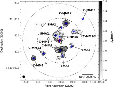
Figure 2. Map of the 1.3 mm continuum emission towards the section of NGC 2264-C observed with the SMA. The grey-scale shows the SMA 1.3 mm continuum emission from 0 to 0.16 Jy beam−1; the peak flux in the field is 0.159 Jy beam−1. The black contours represent (3, 5, 10, 20, 30, 40, 50, 60, 70, 80)×σ=2 mJy beam−1. The peak continuum positions for the 10 leaves (millimetre continuum peaks) identified in the dendrogram are marked with blue pluses (+) and labelled SMA – for new detections and C-MM —for previously detected sources. The blue triangle marks the peak position of the possible millimetre continuum peak C-MM5b. The red star represents the position of AFGL 989-IRS1, taken from the 2MASS data in the RMS survey, and the blue cross (x) marks the position of C-MM11 from Peretto et al. (2007). The black dashed circle represents the FWHP of the SMA primary beam, and the outer black dotted circle represents the 10 per cent power level of the SMA primary beam. The SMA synthesized beam (3.06×2.69 arcsec, PA= −69.3) is shown at lower left.
3 R E S U LT S
3.1 1.3 mm continuum emission
The SMA 1.3 mm continuum image is presented in Fig.2. The
structure of the 1.3 mm emission was characterized through the
implementation of dendrograms (Rosolowsky et al.2008).
Dendro-grams or structure tree diaDendro-grams can be used to define hierarchical structure in clouds. The dendrogram tree structures are comprised of three main components: a trunk, branches and leaves, which correspond to increasing levels of intensity in the data set. We set the minimum threshold intensity required to identify a parent tree
structure (e.g. trunk) to be 4σ (in the continuum image prior to
correction for the primary beam response;σ∼2 mJy beam−1) and
a minimum area of 18 contiguous pixels (the equivalent area of the synthesized beam). Further nested substructures (i.e. branches and
leaves) require an additional 1σ increase in intensity, again over a
minimum of 18 contiguous pixels. To compute the dendrogram, we
have used thePYTHONimplementation astrodendro.7
We identify 10 millimetre continuum sources in our SMA 1.3 mm image with the dendrogram analysis, of which four are new
detec-tions (labelled SMA1-SMA4 in Fig.2). The other six 1.3 mm
con-7This research made use of astrodendro, a
PYTHONpackage to compute dendrograms of astronomical data (http://www.dendrograms.org/).
tinuum sources have been previously reported (Ward-Thompson
et al.2000; Peretto et al.2006,2007) and are labelled in Fig.2
according to the naming scheme of Peretto et al. (C-MM-). Of the ten 1.3 mm continuum sources identified in the dendrogram analy-sis, five are found as separate, independent parent structures with no substructure, and five are found nested into two tree structures. The two nested structures are comprised of C-MM4 and SMA4,
and of C-MM5, SMA1, and SMA2, respectively (see Fig.3for
an example of nested structure). The parameters of the millimetre continuum sources (e.g. peak intensity, integrated flux density, and
effective radius) were extracted using the analysis code
Comput-ing Dendrogram Statistics8and the CASAVIEWER tool, and are
presented in Table1. All properties are estimated from the primary
beam corrected 1.3 mm continuum image using a 3σmask derived
from the continuum image prior to correction for the primary beam response. This approach was taken to avoid including noise in the parameter estimates for millimetre continuum sources far from the pointing centre.
We detect all of the previously identified millimetre continuum peaks within the FWHP of our SMA primary beam. Of the sources
reported by Peretto et al. (2006) and Peretto et al. (2007) that fall
8This research made use of Astropy, a community-developed core PYTHON package for astronomy (Astropy Collaboration et al.2013).
at University of St Andrews on April 11, 2016
http://mnras.oxfordjournals.org/
Figure 3. Examples of dendrogram tree structure for C-MM5, C-MM12, SMA1, and SMA2. The left-hand panel shows the 1.3 mm continuum image, corrected for the primary beam response, in grey-scale, overlaid with 3σ contours from the 1.3 mm continuum image prior to correction for the primary beam. These contours correspond to structures identified in the dendrogram analysis (Section 3.1). Structures are identified using a minimum threshold of 4σ (1σ =2 mJy beam−1) and a minimum number of 18 contiguous pixels, with a step increase of 1σ for further substructure to be identified. The black contours (left-hand panel) and corresponding black lines (tree diagram, right-hand panel) show an example of a parent tree structure with further substructure (in this case the structure containing C-MM5, SMA1, and SMA2). The green contour represents an additional branch within this structure, which hosts two cores, C-MM5 and SMA2. The red contours (left-hand panel) and corresponding red lines (tree diagram, right-hand panel) denote the highest level of a parent structure or of an independent structure with no further substructure if present. C-MM12 shows only parent structure and has no further substructure.
Table 1. Properties of millimetre continuum sources.
Sourcea J2000.0 coordinatesb J2000.0 coordinatesc R
effd Ipeake Sνf
α(h m s) δ(◦ ) α(h m s) δ(◦ ) (pc) (mJy beam−1) (mJy)
C-MM3 06 41 12.31 +09 29 11.50 06 41 12.28 +09 29 11.96 0.011 370 395
C-MM4 06 41 10.08 +09 29 21.70 06 41 09.95 +09 29 21.40 0.017 185 496
C-MM5 06 41 10.15 +09 29 33.70 06 41 10.14 +09 29 35.87 0.012 62 131
C-MM10 06 41 08.94 +09 29 44.56 06 41 08.75 +09 29 44.24 0.015 37 113
C-MM12 06 41 09.59 +09 29 54.64 06 41 09.63 +09 29 54.62 0.013 209 274
C-MM13 06 41 11.47 +09 29 17.47 06 41 11.51 +09 29 18.00 0.0099 34 53
SMA1 06 41 10.00 +09 29 49.25 06 41 10.12 +09 29 47.97 0.0079 15 21
SMA2 06 41 10.46 +09 29 39.66 06 41 10.46 +09 29 39.16 0.0057 27 26
SMA3 06 41 09.11 +09 29 26.50 06 41 09.16 +09 29 27.38 0.0093 17 31
SMA4 06 41 09.88 +09 29 14.53 06 41 09.88 +09 29 14.85 0.0053 48 36
Notes.aSources identified in the dendrogram analysis: C-MM – denotes previously known/named millimetre sources (Peretto et al.
2006,2007); SMA – denotes new 1.3 mm detections.
bPosition of millimetre continuum peak.
cPosition of intensity-weighted centroid, computed usingComputing Dendrogram Statistics(Astropy Collaboration et al.2013). dEffective radius, computed from the total leaf area usingComputing Dendrogram Statistics(Astropy Collaboration et al.2013),
throughReff=√Area/πand assuming the distance of 738pc to NGC 2264-C.
ePeak intensity of 1.3 mm continuum emission, corrected for the primary beam response.
fIntegrated 1.3 mm flux density, measured from the primary-beam-corrected continuum image using CASAVIEWER and the 3σ
mask from the dendrogram computed from the uncorrected image (see Section 3.1). For sources which are nested within parent structures (e.g. C-MM5, SMA1, and SMA2), only the flux from within the highest level of that structure (e.g. the leaves) is extracted (see the red contours in Fig.3).
within the field of view shown in Fig.2, only C-MM11 – which lies
outside the 20 per cent power level of the SMA primary beam – is not detected in our SMA image. Our non-detection of C-MM11 is also consistent with the relative intensities of the millimetre
contin-uum sources reported by Peretto et al. (2006, 1.2 mm IRAM 30-m
observations): C-MM11 is the weakest Peretto et al. source within
our SMA field (Fig.1).
Our four new detections SMA1, SMA2, SMA3, and SMA4 have the lowest integrated flux densities of the 10 millimetre contin-uum sources: the brightest new detections (SMA3 and SMA4) have integrated flux densities that are approximately half that of the weakest previously reported source (C-MM13) in our SMA image
(Table1). This is consistent with SMA1-SMA4 not having been
reported based on previous observations. We note that SMA4 is
visible as a 3σcontour in fig. 1 of Peretto et al. (2007, PdBI 3.2 mm
observations), but was considered a marginal detection and not studied further.
Inspecting the continuum map by eye reveals an additional mil-limetre continuum peak not identified by the dendrogram analysis. We separate C-MM5 into two cores: one at the peak position for
C-MM5 tabulated in Table1, and a second∼4.5 arcsec north (see
Fig.2). The intensity of this second peak surpasses the dendrogram
threshold for substructure; however, the number of contiguous pix-els is below the set limit, so the leaf is merged into C-MM5. If the number of contiguous pixels required is reduced to 77 per cent of the area of the synthesized beam, C-MM5 is separated into two
at University of St Andrews on April 11, 2016
http://mnras.oxfordjournals.org/
Table 2. Molecular line transitions detected towards millimetre continuum peaks in NGC 2264-C. Species Transition Frequencya E
uppera Detectedb
(GHz) (K) CMM3 CMM4 CMM5 CMM10 CMM12 CMM13 CMM5b SMA1 SMA2 SMA3 SMA4 LSB
CH3OH 5(1, 4)−4(2, 2) 216.946 55.9 N Y N N N N N N N N N
SiO (5−4) 217.105 31.3 Y Y N N Y N Y N N N N
DCN (3−2) 217.239 20.9 N Y Y Y N N Y N Y N N
c-C3H2c 616−505 217.822 38.6 N Y N N Y N N N Y N N
c-C3H2c 606−515 217.822 38.6 N Y N N Y N N N Y N N
c-C3H2 514−523 217.940 35.4 N Y N N N N N N Y N N
H2CO 3(0, 3)−2(0, 2) 218.222 21.0 Y Y N Y Y N Y N Y Y N
HC3N (24−23) 218.324 131.0 N Y Y N N N Y N N N N
CH3OH 4(2, 2)−3(1, 2) 218.440 45.5 N Y N N N N N N N Y N
H2CO 3(2, 2)−2(2, 1) 218.476 68.1 N Y N N N N N N N Y N
H2CO 3(2, 1)−2(2, 0) 218.760 68.1 Y Y N N Y N Y N Y Y N
OCS (18−17) 218.903 99.8 N Y N N Y N N N N N N
C18O (2−1) 219.560 15.8 N Y N Y N N Y Y Y Y N
SO 6(5)−5(4) 219.949 35.0 N Y Y N Y N Y N Y Y N
CH3OH 8(0, 8)−7(1, 6) E 220.078 96.6 N Y N N N N N N N N N
CH3CN (124−114) 220.679 183.3 N N Yd N N N N N N N N
CH3CN (123−113) 220.709 133.3 N Yd Yd N N N N N N N N
CH3CN (122−112) 220.730 97.4 N Yd Yd N N N N N N N N
CH3CNe (121−111) 220.743 76.0 N Y Y N N N N N N N N
CH3CNe (120−110) 220.747 68.8 N Y Y N N N N N N N N
USB
CH3OH 8(−1, 8)−7(0, 7) E 229.759 89.1 N Y N N N N N N N Y N
CH3OH 3(−2, 2)−4(−1, 4) E 230.027 39.8 N Y N N N N N N N N N
OCS (19−18) 231.061 110.8 N Y N N N N N N N N N
13CS (5−4) 231.221 33.29 N Y N N N N N N Y N N
Notes.aFrom Splatalogue (http://www.splatalogue.net/), M¨uller et al. (2005).
bY: detected at≥5σ, N: undetected (no emission at≥5σ). All measurements were made from image cubes corrected for the primary beam response, and a
detection was determined from the spectra extracted from those beam corrected image cubes. Thus, for sources far from the pointing centre such as C-MM3, the rms noise is higher.
cThese components are blended in the spectra and cannot be separated. dCH
3CN components where emission is<5σbut>3σ.
eThese CH
3CN components are blended in the spectra: ‘Y’ indicates emission>5σfor the blended line. See Table3for line fits.
leaves by the dendrogram analysis. Inspection of the molecular line emission also indicates these two leaves may be separate objects (Section 3.2). We therefore suggest that the northern leaf (hereafter C-MM5b) and C-MM5 are distinct millimetre continuum peaks, which we are unable to unequivocally separate at the resolution of our SMA data.
3.2 Molecular line emission
We detect molecular line emission in 23 transitions of 13 species
above 5σ with the SMA, including SiO, CO and its isotopologues
(13CO and C18O), SO, OCS, H
2CO, CH3OH, DCN, c-C3H2,13CS,
HC3N, and CH3CN. All lines detected at>5σhaveEupperbetween
∼16 and 131 K. Table2lists the species, transition, rest frequency,
Eupper, and whether the line is detected at>5σtowards the millime-tre continuum peak of each of the 11 cores (including C-MM5b,
see Section 3.1). Table3presents the parameters (peak line
inten-sity, line centre velocity, linewidth, and integrated line intensity)
obtained from single Gaussian fits to lines detected at>5σ, at each
millimetre continuum peak. No fits are presented for12CO and
13CO due to the complexity of the line profiles, which are strongly
affected both by self-absorption and by artefacts from poorly
im-aged large-scale emission;12CO and13CO are similarly excluded
from Table2.
Fig. 4 presents integrated intensity maps for all detected
transitions, including 12CO and 13CO. The velocity range over
which emission is integrated is determined for each transition, to
encompass all channels with emission above 3σ. As shown in
Fig.4, the morphology of the detected line emission is complex.
For many transitions, the spatial morphology of the line emission differs markedly from that of the millimetre continuum. The emis-sion in the integrated intensity maps falls into three main categories: (i) ‘compact’ molecular line emission that directly traces
millime-tre continuum peaks, which includes emission from CH3CN, OCS
(18−17) and OCS (19−18), HC3N, and the CH3OH 5(1, 4)−4(2, 2),
CH3OH 8(0, 8)−7(1, 6) E and CH3OH 3(−2, 2)−4(−1, 4) E
transi-tions; (ii) ‘diffuse’ molecular line emission that overlaps but may not be clearly associated with millimetre continuum emission (e.g. may
differ in morphology), which includes emission from c-C3H2, DCN
and C18O; and (iii) spatially extended molecular line emission that
is more likely associated with outflows, which includes emission
from SiO, SO, H2CO, and the CH3OH 4(2, 2)−3(1, 2) and CH3OH
8(−1, 8)−7(0, 7) E transitions. Emission from13CS appears to fall
into both the ‘compact’ (i) and ‘diffuse’ (ii) categories. As shown
in Fig.4, the velocity-integrated12CO and13CO emission extends
across much of the field,12CO and13CO are therefore not included
in these categories; high-velocity12CO, however, traces outflows,
as discussed in Section 3.2.2.
A distinct feature, which we have labelled the ‘ridge’, is also
evident in Fig.4. The ridge is associated with the strongest H2CO
emission in the field, as well as the strongest emission in several
CH3OH transitions. While the southern edge of the ridge overlaps
at University of St Andrews on April 11, 2016
http://mnras.oxfordjournals.org/
Table 3. Gaussian fits to molecular lines detected at millimetre continuum peaks.
Species Transition Frequency Eupper Fitted line parameters
Peak intensitya V
centrea Linewidtha
S dva
(GHz) (K) (Jy beam−1) (km s−1) (km s−1) (Jy beam−1km s−1) C-MM3
H2COb 3(0, 3)−2(0, 2) 218.222 21.0 0.91 (0.11) 6.60 (0.22) 3.93 (0.54) 3.80 (0.49) H2COb 3(0, 3)−2(0, 2) 218.222 21.0 0.44 (0.08) −6.50 (0.33) 4.72 (0.98) 2.22 (0.40)
H2CO 3(2, 1)−2(2, 0) 218.760 68.1 0.58 (0.11) 8.22 (0.25) 2.68 (0.62) 1.66 (0.36)
C-MM4
CH3OH 5(1, 4)−4(2, 2) 216.946 55.9 0.25 (0.03) 8.88 (0.15) 3.70 (0.35) 0.98 (0.12)
SiOc (5−4) 217.105 31.3 0.22 (0.03) 15.04 (0.41) 5.33 (0.97) 1.26 (0.30)
DCN (3−2) 217.239 20.9 0.87 (0.04) 8.53 (0.08) 3.54 (0.19) 3.29 (0.23)
c-C3H2 616−505 217.822 38.6 0.55 (0.03) 7.77 (0.06) 2.54 (0.15) 1.50 (0.08)
c-C3H2 514−523 217.940 35.4 0.24 (0.03) 8.70 (0.19) 2.92 (0.46) 0.74 (0.11)
H2CO 3(0, 3)−2(0, 2) 218.222 21.0 1.75 (0.03) 7.62 (0.03) 3.3 (0.07) 6.14 (0.11)
HC3N (24−23) 218.324 131.0 0.21 (0.03) 8.11 (0.20) 3.88 (0.49) 0.85 (0.14)
CH3OH 4(2, 2)−3(1, 2) 218.440 45.5 0.51 (0.03) 8.72 (0.11) 3.39 (0.26) 1.83 (0.13)
H2CO 3(2, 2)−2(2, 1) 218.476 68.1 0.55 (0.03) 7.82 (0.11) 3.85 (0.26) 2.24 (0.14)
H2CO 3(2, 1)−2(2, 0) 218.760 68.1 0.80 (0.03) 8.11 (0.06) 3.57 (0.14) 3.06 (0.11)
OCS (18−17) 218.903 99.8 0.21 (0.02) 8.84 (0.33) 6.29 (0.89) 1.43 (0.18)
C18O (2−1) 219.560 15.8 2.59 (0.05) 8.03 (0.18) 2.38 (0.04) 6.57 (0.11)
SO 6(5)−5(4) 219.949 35.0 1.32 (0.05) 8.16 (0.05) 3.04 (0.13) 4.28 (0.17)
CH3CN (123−113) 220.709 133.3 0.10 (0.01) 5.77 (0.51) 2.76 (1.08) 0.28 (0.11)
CH3CN (122−112) 220.730 97.4 0.14 (0.01) 5.32 (0.4) 2.46 (0.80) 0.37 (0.10)
CH3CNd (121−111) 220.743 76.0 0.21 (0.01) 7.69 (0.28) 1.61 (0.53) 0.37 (0.10)
CH3CNd (120−110) 220.747 68.8 0.16 (0.01) 7.34 (0.29) 2.34 (0.59) 0.40 (0.10)
CH3OH 8(0, 8)−7(1, 6) E 220.078 96.6 0.21 (0.03) 7.96 (0.30) 4.70 (0.73) 1.07 (0.15) CH3OH 8(−1, 8)−7(0, 7) E 229.759 89.1 0.36 (0.03) 8.29 (0.15) 4.06 (0.37) 1.54 (0.13) CH3OH 3(−2, 2)−4(−1, 4) E 230.027 39.8 0.22 (0.03) 8.32 (0.28) 4.35 (0.68) 1.02 (0.15)
OCS (19−18) 231.061 110.8 0.27 (0.03) 8.42 (0.23) 4.07 (0.55) 1.19 (0.15)
13CS (5−4) 231.221 33.29 0.26 (0.04) 7.61 (0.30) 4.28 (0.74) 1.16 (0.19)
C-MM5
DCN (3−2) 217.239 20.9 0.13 (0.02) 9.54 (0.22) 2.09 (0.56) 0.28 (0.10)
HC3N (24−23) 218.324 131.0 0.25 (0.02) 9.51 (0.08) 2.65 (0.28) 0.70 (0.06)
SOb 6(5)−5(4) 219.949 35.0 0.55 (0.05) 7.22 (0.70) 6.13 (1.73) 3.57 (1.06)
SOb 6(5)−5(4) 219.949 35.0 0.33 (0.01) 13.2 (0.08) 3.89 (0.21) 1.35 (0.09)
CH3CN (124−114) 220.679 183.3 0.12 (0.03) 8.82 (0.30) 2.68 (0.69) 0.34 (0.11)
CH3CN (123−113) 220.709 133.3 0.10 (0.02) 5.59 (0.46) 2.83 (1.20) 0.30 (0.10)
CH3CN (122−112) 220.730 97.4 0.11 (0.02) 7.26 (0.48) 4.05 (0.98) 0.49 (0.11)
CH3CNd (121−111) 220.743 76.0 0.12 (0.02) 7.51 (0.64) 2.78 (1.26) 0.35 (0.18)
CH3CNd (120−110) 220.747 68.8 0.20 (0.02) 8.51 (0.27) 3.61 (0.50) 0.78 (0.12)
C-MM10
DCN (3−2) 217.239 20.9 0.38 (0.05) 7.80 (0.15) 2.07 (0.33) 0.84 (0.17)
H2CO 3(0, 3)−2(0, 2) 218.222 21.0 1.09 (0.11) 7.71 (0.09) 1.59 (0.19) 1.85 (0.30)
C18O (2−1) 219.560 15.8 0.25 (0.04) 7.83 (0.26) 3.56 (0.61) 0.96 (0.22)
C-MM12
SiOc (5−4) 217.105 31.3 0.65 (0.05) 10.93 (0.16) 4.36 (0.47) 3.03 (0.28)
c-C3H2 616−505 217.822 38.6 0.31 (0.06) 9.34 (0.20) 1.86 (0.38) 0.61 (0.12)
H2CO 3(0, 3)−2(0, 2) 218.222 21.0 0.57 (0.09) 11.18 (0.28) 3.55 (0.66) 2.17 (0.54) H2CO 3(2, 1)−2(2, 0) 218.760 68.1 0.20 (0.02) 10.86 (0.14) 2.97 (0.33) 0.64 (0.10)
OCS (18−17) 218.903 99.8 0.22 (0.02) 8.49 (0.18) 3.96 (0.42) 0.94 (0.13)
SOb 6(5)−5(4) 219.949 35.0 0.47 (0.06) 10.85 (0.29) 4.51 (0.70) 2.25 (0.46)
SOb 6(5)−5(4) 219.949 35.0 0.25 (0.03) 28.90 (0.28) 5.85 (0.67) 1.62 (0.24)
SMA1
C18O (2−1) 219.560 15.8 0.67 (0.08) 9.92 (0.11) 2.19 (0.29) 1.59 (0.28)
SMA2
DCN (3−2) 217.239 20.9 0.36 (0.04) 9.95 (0.18) 3.23 (0.42) 1.23 (0.21)
c-C3H2e 616−505 217.822 38.6 0.27 (0.03) 9.42 (0.13) 2.78 (0.31) 0.81 (0.12)
c-C3H2 514−523 217.940 35.4 0.25 (0.03) 10.38 (0.15) 2.54 (0.34) 0.67 (0.12)
H2CO 3(0, 3)−2(0, 2) 218.222 21.0 0.56 (0.04) 9.72 (0.10) 3.31 (0.25) 2.00 (0.20)
H2CO 3(2, 1)−2(2, 0) 218.760 68.1 0.19 (0.03) 9.88 (0.23) 2.89 (0.53) 0.58 (0.14)
C18O (2−1) 219.560 15.8 1.73 (0.06) 9.68 (0.05) 2.70 (0.11) 4.97 (0.27)
SO 6(5)−5(4) 219.949 35.0 0.80 (0.02) 9.52 (0.02) 2.16 (0.06) 1.82 (0.06)
13CS (5−4) 231.221 33.29 0.39 (0.05) 9.52 (0.12) 2.06 (0.28) 0.85 (0.15)
at University of St Andrews on April 11, 2016
http://mnras.oxfordjournals.org/
Table 3 – continued
Species Transition Frequency Eupper Fitted line parameters
Intensitya V
centrea Widtha
S dva
(GHz) (K) (Jy beam−1) (km s−1) (km s−1) (Jy beam−1km s−1) SMA3
H2CO 3(0, 3)−2(0, 2) 218.222 21.0 2.48 (0.08) 8.96 (0.08) 4.59 (0.18) 12.08 (0.63) CH3OH 4(2, 2)−3(1, 2) 218.440 45.5 1.08 (0.07) 8.55 (0.08) 2.56 (0.20) 2.94 (0.30)
H2CO 3(2, 2)−2(2, 1) 218.476 68.1 1.30 (0.04) 8.83 (0.05) 3.47 (0.12) 4.80 (0.21)
H2CO 3(2, 1)−2(2, 0) 218.760 68.1 1.20 (0.04) 8.81 (0.05) 3.56 (0.12) 4.58 (0.12)
C18O (2−1) 219.560 15.8 0.39 (0.04) 8.83 (0.23) 4.84 (0.54) 2.01 (0.30)
SOe 6(5)−5(4) 219.949 35.0 0.43 (0.06) 9.93 (0.41) 6.26 (0.96) 2.84 (0.57)
CH3OH 8(−1, 8)−7(0, 7) E 229.759 89.1 0.97 (0.04) 8.60 (0.07) 3.40 (0.17) 3.52 (0.23) C-MM5b
SiO (5−4) 217.105 31.3 0.34 (0.03) 14.61 (0.16) 4.15 (0.37) 1.49 (0.17)
DCN (3−2) 217.239 20.9 0.94 (0.05) 9.31 (0.07) 2.52 (0.17) 2.51 (0.22)
H2CO 3(0, 3)−2(0, 2) 218.222 21.0 0.68 (0.06) 8.93 (0.09) 2.22 (0.22) 1.60 (0.21)
HC3N (24−23) 218.324 131.0 0.44 (0.03) 8.97 (0.07) 2.11 (0.17) 0.99 (0.11)
H2CO 3(2, 1)−2(2, 0) 218.760 68.1 0.12 (0.02) 9.63 (0.22) 4.11 (0.52) 0.54 (0.09)
C18O (2−1) 219.560 15.8 1.54 (0.08) 9.28 (0.06) 2.39 (0.13) 3.92 (0.29)
SOb 6(5)−5(4) 219.949 35.0 0.39 (0.07) 9.83 (0.17) 2.18 (0.47) 0.90 (0.24)
SOb 6(5)−5(4) 219.949 35.0 0.14 (0.03) 15.32 (0.21) 3.12 (0.51) 0.48 (0.10)
Notes.aFormal errors from the single Gaussian fits are given in the brackets.
bTwo distinct velocity components are present in the spectrum; a single Gaussian fit is reported for each component.
cTwo velocity components appear to be present in the spectrum, but are not sufficiently well separated in velocity to be fit separately. The reported fit is for the
stronger component.
dThek=0 and 1 CH
3CN components are blended in the spectra. The reported parameters are from multiple-Gaussian fits using theGILDAS CLASSpackage.
eComplex line profile, not well fit by a single Gaussian.
SMA3, the majority of the ridge structure does not appear to be associated with a millimetre continuum source. The nature of this intriguing feature is discussed in Section 4.2.
3.2.1 Line emission associated with millimetre continuum sources: systemic velocity estimates
As shown in Fig.4, compact molecular line emission that peaks at
the millimetre continuum peaks is seen in only a few lines (OCS,
CH3CN, HC3N, and the 216.946 GHz, 220.078, and 230.027 GHz
CH3OH transitions), and only towards MM4, MM5, and
C-MM5b (not all of these lines are detected towards all three sources;
see Table2). For these sources, we present estimates of thevLSR’s of
the individual millimetre continuum cores in Table4, based on the
fits (Table3) to lines that exhibit spatially compact emission. We
note that for CH3CN, the ladder transitions with a detection<5σ
are excluded from thevLSRestimates.
DCN and c-C3H2exhibit more extended emission (which we refer
to as ‘diffuse’) that is coincident with, and morphologically simi-lar to, the millimetre continuum emission of C-MM4 and SMA2. For C-MM4, in particular, the similar morphologies of the line and millimetre continuum emission suggest that this more extended molecular line emission is associated with the millimetre contin-uum source. Strong DCN emission is also detected in the vicinity of C-MM5 and C-MM5b, but in this case the morphology of the line emission differs from that of the millimetre continuum, so it is not clear that the DCN emission is directly associated with the
con-tinuum source(s). Table4presents estimates of corevLSR’s based
on fits to lines that exhibit ‘diffuse’ emission (including C18O as
well as DCN and c-C3H2) and are detected at the position of a
given core’s millimetre continuum peak. We emphasize that while
this approach allows us to estimatevLSR’s for more sources, the
results must be treated with greater caution than the estimates based
on compact molecular line emission. The morphology of the C18O
emission, for example, does not match that of the millimetre
con-tinuum, suggesting that the detected C18O may not arise from the
dense gas of the millimetre continuum cores. OurvLSRestimates
exclude lines that likely trace outflows and exhibit clearly extended
emission (e.g. SiO, SO, H2CO, and the remaining CH3OH lines).
ThevLSR’s of the millimetre continuum sources, estimated as
described above, range from∼7.8 to 9.9 km s−1. For C-MM4 and
C-MM5 (for which we have the most data from line fits, see Tables3
and4), thevLSRestimates based on compact and ‘diffuse’ tracers
differ by up to∼1 km s−1(for C-MM5), and the standard
devia-tion of thevLSR’s measured from individual lines is∼0.5 km s−1
(Table4).
Towards C-MM3, C-MM13, SMA1, and SMA4 no emission is detected from lines that exhibit either ‘compact’ or ‘diffuse’
mor-phology. As a result, we cannot estimate thevLSR’s of these sources
from our SMA data. vLSR estimates for C-MM3 and C-MM13
are of particular interest, given the outflow activity near C-MM3 (Section 3.2.2) and the velocity gradient reported by Peretto et al.
(2007) in NGC 2264-C (spanning C-MM2, C-MM3, C-MM13,
and C-MM4). Since we are unable to estimatevLSR’s for several
continuum sources from our SMA data (and have robust estimates based on compact molecular line emission for only a small minor-ity), we adopt the following approach. For C-MM4, where we have the most detected compact emission, we use our estimate of the
vLSRof 8.3 km s−1for the remaining analysis. For MM3 and
C-MM13, we adopt thevLSR’s reported by Peretto et al. (2007) based
on N2H+(1−0) emission (Table4). For the remaining millimetre
continuum sources, we adopt the averagevLSRfrom our SMA data
(averaged across all cores, for both compact and diffuse tracers)
of 8.9 km s−1. We note that for C-MM10 and C-MM5b, we have
at University of St Andrews on April 11, 2016
http://mnras.oxfordjournals.org/
multiple, consistent velocity measurements from our SMA data (though for C-MM10 only from ‘diffuse’ tracers); however, as these
cores show no evidence of outflow activity, we adopt the threevLSR’s
described above for simplicity in plotting composite maps of red
and blueshifted emission (e.g. Fig.6). ThevLSRadopted for each
continuum peak, and used throughout the remainder of this paper,
is given in Table4.
3.2.2 Extended and high velocity molecular line emission: molecular outflows
As shown in Fig.4, several species are characterized by collimated,
extended emission: SiO, SO, CH3OH, H2CO, and12CO. The two
[image:9.595.68.534.148.661.2]most prominent collimated emission features in the integrated in-tensity maps (both elongated N-S) appear to be centred on C-MM3
Figure 4. SMA integrated intensity maps (green contours) of detected molecular lines, overlaid on the 1.3 mm continuum emission (grey-scale and black contour, contour level 3σ =6 mJy beam−1). The integrated velocity range is given in the top-left corner of each panel, along with the molecule and line rest frequency.Eupperfor the transition and the peak and rms of each map (both in Jy beam−1km s−1) are given at upper right in each panel. Blue pluses (+) mark the positions of the millimetre continuum peaks from Table1, and the blue triangle marks the position of C-MM5b (see Section 3.1). Contour levels for the integrated intensity maps are from 3σto peak in steps of 2σ. Panel (p) shows the CH3CN emission integrated over thek=0–4 components and thus the velocity range and frequency is not given.
at University of St Andrews on April 11, 2016
http://mnras.oxfordjournals.org/
Figure 4 – continued
and C-MM12. To investigate the nature of the extended molecular line emission, and its relation to outflows previously reported based on lower angular resolution data, we analyse its velocity structure. To identify potential outflow axes, we use our high-resolution SMA observations of the well-known outflow tracer SiO (e.g. Gusdorf
et al.2008a,b; Guillet et al.2009; Leurini et al. 2014, and
refer-ences therein).
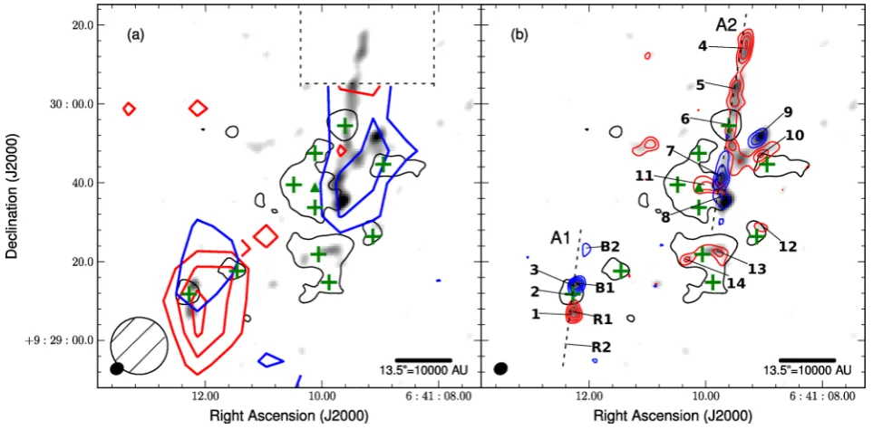
Fig. 5 presents integrated intensity maps of the red- and
blueshifted SiO emission observed with the SMA (SiO (5−4),
reso-lution∼3 arcsec) and the JCMT (SiO (8−7), resolution∼15 arcsec).
We compare the SMA and JCMT data to test whether the spatial filtering of the SMA misses any large-scale active outflows (which would be seen in SiO emission with the JCMT). The JCMT
ob-servations (Fig.5a) reveal two potential outflow systems: one
en-compassing both C-MM3 and C-MM13 (with the peak emission nearest to C-MM3), and a second that intersects both C-MM10 and C-MM12. In the second system, only blueshifted emission is de-tected with the JCMT; however, receiver H14 was not operational during our observations, resulting in a gap in the JCMT map north
of C-MM12. Fig.5(b) presents the higher spatial resolution SMA
SiO (5−4) data. With the SMA, the SiO emission near C-MM3 and
C-MM13 is clearly resolved, revealing a single bipolar outflow
centred on C-MM3 (outflow axis A1, Fig. 5b). The red and
blueshifted lobes are spatially well separated and are centred on
the continuum source, indicating that the high-velocity SiO (5−4)
emission traces a bipolar molecular outflow. The second potential outflow system identified in the JCMT data, towards C-MM12 and C-MM10, splits into multiple components at the higher spatial
res-olution of the SMA observations. As shown in Fig.5(b), the SMA
data reveal a collimated, bipolar outflow centred on C-MM12 (axis
A2, Fig.5b): as in the C-MM3 outflow, the red and blueshifted lobes
are spatially well separated and centred on the millimetre contin-uum source. For both outflows, the sense of the velocity gradient is consistent in the SMA and JCMT observations (e.g. the blueshifted lobe is north of C-MM3, and the redshifted lobe south of C-MM3, in both the SMA and JCMT maps). The fact that our SMA SiO data recover (and resolve) both of the SiO outflows identified with the JCMT is strong evidence that the SMA is not ‘missing’ large-scale active outflows.
In addition to the two clear outflows driven by C-MM3 and C-MM12 along axes A1 and A2, there are several additional
com-ponents of SiO emission present in the field, labelled 9–14 in Fig.5.
To the north of C-MM10, red- and blueshifted emission are present (components 9 and 10). Redshifted emission also extends through
at University of St Andrews on April 11, 2016
http://mnras.oxfordjournals.org/
Table 4. Systemic velocity estimates for 1.3 mm continuum sources.
Source vLSR(km s−1)
Compacta Diffuseb N
2H+c Adoptedd
C-MM3 – – 7.1 7.1
C-MM4 8.2 (0.5) 8.3 (0.4) 8.9 8.3
C-MM5 8.5 (1.0) 9.5 – 8.9
C-MM10 – 7.8 (0.02) – 8.9
C-MM12 8.5 9.3 – 8.9
C-MM13 – – 8.2 8.2
SMA1 – 9.9 – 8.9
SMA2 – 9.8 (0.4) – 8.9
SMA3 – 8.8 – 8.9
SMA4 – – – 8.9
C-MM5b 9.0 9.3 (0.02) – 8.9
Notes.aAverage v
LSR estimates from molecular lines categorized as ex-hibiting ‘compact’ emission (see Section 3.2) and includes emission from CH3CN (note only CH3CN transitions with>5σdetections are included), OCS, HC3N, and CH3OH 5(1, 4)−4(2, 2), CH3OH 8(0, 8)−7(1, 6) E, and CH3OH 3(−2, 2)−4(−1, 4) E. Note that not all of these lines are detected at>5σtowards each core; see Table2. Furthermore,13CS is not used in the
vLSRestimate for ‘compact’ emission as it also displays diffuse emission. The standard deviation is given in the brackets. If no value is given, emission was detected only in one transition.
bAveragev
LSR estimates from molecular lines categorized as exhibiting ‘diffuse’ emission (see Section 3.2) and includes emission from C18O, DCN, and c-C3H2. Again13CS is not used in thevLSRestimate for ‘diffuse’ tracers as it also appears to trace compact emission. Note that not all of these lines are detected towards each core; see Table2. The standard deviation is given in the brackets. If no value is given, emission was detected only in one transition.
cTaken from Peretto et al. (2007). dv
LSRadopted for each core for the remainder of the analysis.
the blueshifted axis of A2 to C-MM5b (component 11). In addi-tion, extended redshifted SiO emission is observed towards C-MM4 (components 13 and 14) and redshifted emission is found coinci-dent with SMA3 (component 12). The nature of this additional SiO emission is unclear.
To further explore the nature and structure of the high-velocity outflow emission in NGC 2264-C, we consider four velocity regimes
(e.g. Santiago-Garc´ıa et al. 2009): systemic (vLSR ± 3 km s−1),
standard high velocity (SHV, vLSR±3 to 10 km s−1),
intermedi-ate high velocity (IHV,vLSR±10–30 km s−1), and extremely high
velocity (EHV, vLSR± 30–50 km s−1). Fig. 6presents SMA
in-tegrated intensity maps for the systemic, SHV, and IHV regimes
for SiO (5−4), SO (6(5)−5(4)), H2CO (3(0, 3)−2(0, 2)), and
12CO (2−1). These are the only four transitions in which
emis-sion is detected at velocities >10 km s−1 from the v
LSR (e.g. in
the IHV regime). We do not present EHV maps because very
lit-tle EHV emission is detected: the only >3σ emission with|v−
vLSR|>30 km s−1is12CO (2−1) at∼31 km s−1, towards the
red-shifted lobe of the C-MM3 outflow. As described in Section 3.2.1,
above, we adopt a vLSRof 7.1 km s−1for C-MM3 and avLSR of
8.3 km s−1for the region covering C-MM4 (including C-MM13).
For the rest of the region, the velocity ranges are calculated with
re-spect to avLSR=8.9 km s−1(adopted for the other continuum cores,
Section 3.2.1).
Towards the outflow axis A2, low-velocity (systemic) emission
is traced by SiO, SO, and H2CO (as shown in Fig.6). In
con-trast, along axis A1 only H2CO is detected at low velocities. In
addition, two CH3OH lines (CH3OH 4(2,2)−3(1,2) and CH3OH
8(−1,8)−7(0,7)E) exhibit extended emission along the outflow axes
(see Fig.4) only in the systemic and SHV regimes, and so are not
shown in Fig.6. There is also a noticeable extension in the systemic
emission from SO and H2CO running from north-west to south-east
coincident with the components 9–11.
In the SHV regime, collimated red- and blueshifted emission
cen-tred on C-MM3 and C-MM12 is detected in SiO, SO, and H2CO.
The IHV 12CO emission displays a similar morphology,
consis-tent with the SHV and IHV molecular line emission tracing bipolar molecular outflows driven by these two millimetre continuum cores.
(The12CO emission in the SHV regime is affected by poorly imaged
extended structure and confusion with the surrounding cloud,
mak-ing it difficult to identify outflows in12CO in this velocity range.)
Both lobes of the outflow associated with C-MM3 are also detected in the IHV regime in SiO and SO, while only the redshifted lobe of the outflow associated with C-MM12 is detected in IHV SiO, SO,
and H2CO emission (Fig.6).
The additional SiO components (numbered 9–14 in Fig.5) are
also associated with SHV SO and H2CO emission, with the
ex-ception of the redshifted emission towards C-MM4. Redshifted SHV SiO emission is observed towards both C-MM4 and SMA3
(components 12–14), while (redshifted) SO and H2CO emission are
only observed towards SMA3 (component 12). In the IHV regime,
only12CO emission is detected towards these components. While
both redshifted (near SMA3) and blueshifted (south of C-MM4) emission are present, these potential lobes are not centred on a mil-limetre continuum source and it is unclear if they are related to a single outflow. Compared to the two bipolar outflows (along A1 and A2), the velocity extent of the emission towards the additional,
ambiguous SiO components is also more modest. For12CO (2−1),
the maximum redshifted velocity is ∼38, 32, 28, and 24 km s−1
for A1 (C-MM3 outflow, components 1–3), A2 (C-MM12 outflow, components 4–8), towards C-MM10/C-MM5b (components 9–11) and towards C-MM4/SMA3 (components 12–14), respectively. The
minimum velocity for blueshifted12CO emission is−17.2 km s−1
for A1 (C-MM3 outflow) and−2.8 km s−1for A2 (C-MM12
out-flow) and towards C-MM4.
To examine the outflow kinematics in greater detail, Fig. 7
presents SiO, SO, H2CO, and12CO spectra at the positions labelled
in Fig.5, along the potential outflow axes A1 and A2 (numbered
1–8), and towards the additional components (numbered 9–14).
Works by Codella et al. (2014), Tafalla et al. (2010), and Lee et al.
(2010) identified similarities between SiO and SO emission at high
velocities. As shown in Fig.6, SiO and SO exhibit similar
mor-phologies in NGC 2264-C; however, the SiO emission extends to higher absolute velocities compared with the SO emission (e.g. for SiO the maximum red- and blueshifted velocities are 37 and
−20 km s−1, respectively, compared with 32 and−13 km s−1 for
SO). Close examination of the line profiles also reveals a
veloc-ity gradient in12CO towards C-MM4 and SMA3, from redshifted
(component 12) to blueshifted (component 14). This12CO emission
is lower velocity than observed towards axes A1 and A2. The SiO emission is also considerably narrower towards C-MM4 and SMA3 than along axes A1 and A2.
We note that SiO (5−4) emission associated with outflows from
low-mass (proto)stars is unlikely to be detected as extended, col-limated structure in our SMA observations. Scaling the results of
G´omez-Ruiz et al. (2013) and Codella et al. (2014) to the distance
of NGC 2264-C and our SMA beam, we would detect only the
strongest SiO (5−4) emission, and that at the∼4σ–8σ level. We
also note that in both the JCMT and SMA observations, the width of the collimated emission appears to be limited by the size of the beam.
at University of St Andrews on April 11, 2016
http://mnras.oxfordjournals.org/
Figure 5. SiO kinematics. SMA SiO integrated intensity map (grey-scale, integrated over the velocity range−20 to 37 km s−1) overlaid with contours of 1.3 mm continuum emission (black contour, level 3σ=6 mJy beam−1) and blue/redshifted SiO emission from (a) the JCMT (SiO (8−7)) and (b) the SMA (SiO (5−4)). The velocity intervals for the blue/redshifted SiO begin 3 km s−1from thevLSR(vLSR=7.1 km s−1for C-MM3, 8.3 km s−1for C-MM4 and 8.9 km s−1 for C-MM12, see Section 3.2.1) and extend to the maximum outflow velocity. The velocity intervals are the same for the JCMT and SMA data and are: blue: −20 to+4.1 km s−1for C-MM3 (and C-MM13),−1.0 to+5.3 km s−1for C-MM4, and−20 to+5.9 km s−1for C-MM12 (and the other millimetre continuum cores); red:+10.1 to+37 km s−1(C-MM3 and C-MM13),+11.3 to+20 km s−1(C-MM4), and+11.9 to+32 km s−1(C-MM12 and other cores). In both panels, green pluses (+) mark the positions of the 10 millimetre continuum peaks from the dendrogram analysis and the green triangle marks the position of C-MM5b. (a) JCMT SiO (8−7) contour levels: (3,5,7,9)×σ=0.2 K km s−1. The 14.5 arcsec JCMT beam (hatched circle) and the SMA synthesized beam (filled ellipse) are shown at lower left. The dashed rectangle shows the area of missing data from the HARP receiver element H14. (b) SMA SiO (5−4) contour levels: (3,5,7,9)×σ=0.36 Jy beam−1km s−1. The dashed black lines represent the possible outflow axes A1 and A2. The numbered positions 1–14 mark the components discussed in Section 3.2.2, and mark the positions at which the spectra shown in Fig.7were extracted. Positions 1–3 are part of the outflow axis A1, positions 4–8 are part of outflow axis A2, and the remaining positions mark locations of ambiguous SiO emission that is not obviously associated with an outflow. The labels R1, R2, B1, and B2 mark the components of the redshifted and blueshifted outflow lobes of C-MM3 named by Saruwatari et al. (2011).
3.2.3 Candidate millimetre CH3OH masers
A notable feature of Fig.4is the very strong 229.759 GHz CH3OH
emission associated with the ‘ridge’. The 229.759 GHz CH3OH
8(−1, 8)−7(0, 7)E transition is a known class I methanol maser,
first reported towards DR21 (OH) and DR21 west by Slysh,
Kalen-ski˘ı & Val’tts (2002) based on observations with the IRAM
30-m telescope. Probable 30-maser e30-mission in this transition is often seen in SMA observations of massive star-forming regions (e.g.
Fontani et al.2009; Qiu & Zhang2009; Cyganowski et al.2011,
2012; Fish et al. 2011, and references therein). Most recently,
Hunter et al. (2014) directly demonstrated the maser nature of
229.759 GHz CH3OH emission in NGC6334I(N), by showing that
the observed line brightness temperature (TB) is greater than the
upper energy of the transition (Eupper) in very high-resolution SMA
observations.
To investigate the nature of the 229.759 GHz CH3OH emission in
NGC 2264-C, Fig.8presents integrated intensity maps and
corre-sponding line profiles for the CH3OH 8(−1, 8)−7(0, 7) E, CH3OH
8(0, 8)−7(1, 6) E and CH3OH 3(−2, 2)−4(−1, 4) E transitions at
three locations where the CH3OH 8(−1, 8)−7(0, 7) E 229.759 GHz
emission is strongest. These are the ridge, the redshifted outflow lobe of C-MM3, and the redshifted outflow lobe of C-MM12. As
shown in Fig.8, the 229.759 GHz CH3OH emission in the ridge
is more than twice as strong as that towards the redshifted outflow lobe of either C-MM3 or C-MM12.
Like most previous 229 GHz studies (with the notable exception
of Hunter et al.2014), our SMA observations do not have sufficient
angular resolution to establish masing in the 229.759 GHz line based
on its brightness temperature. Slysh et al. (2002) proposed the ratio
of the 229.759 GHz and 230.027 GHz CH3OH lines as a diagnostic
of maser emission, with values of 229.759/230.027>3 indicating
non-thermal 229.759 GHz emission. We note that the 230.027 GHz
line is undetected at all three positions, and the 3σlimits are used to
calculate the line ratios (see Table5for the 3σ limits towards each
position). At two positions in our field, this line ratio is≥3: towards
the redshifted lobe of the C-MM3 outflow, where the ratio is∼3,
and towards the strongest 229.759 GHz emission in the ridge, where
the ratio is considerably higher (∼47). Furthermore, throughout the
ridge the line ratio is consistently>8. While the line ratios towards
the ridge are considerably higher than towards the C-MM3 outflow,
the ridge line ratios fall within the range of line ratios,∼7–100,
found towards the outflow lobes of two extended green objects by
Cyganowski et al. (2011). By comparison, the line ratio towards the
C-MM4 continuum peak is<2, consistent with thermal emission
from warm gas (Section 4.1.1).
Table5presents fits to the 220.078, 229.759, and 230.027 GHz
CH3OH lines at the three positions shown in Fig.8. Emission from
229 GHz CH3OH masers often coincides spatially and spectrally
with emission in lower frequency class I CH3OH maser
transi-tions (e.g. Fish et al.2011; Cyganowski et al.2011,2012). Class
I CH3OH maser emission, in the form of the 44 GHz transition,
at University of St Andrews on April 11, 2016
http://mnras.oxfordjournals.org/
Figure 6. Integrated intensity maps (coloured contours) of emission at systemic (left-hand column), SHV (middle column) and IHV (right-hand column) velocities for the indicated transitions, overlaid on the SMA 1.3 mm continuum image (grey-scale and black contour, contour level 3σ =6 mJy beam−1). ‘Systemic’ is defined asvLSR±3 km s−1(green contours), SHV asvLSR±3–10 km s−1, and IHV asvLSR±>10 km s−1(where red and blue contours represent the red and blueshifted emission, respectively). The maps shown are composites, with an adoptedvLSRof 7.1 km s−1for C-MM3, 8.3 km s−1 for C-MM4 (including the vicinity of C-MM13), and 8.9 km s−1for the remainder of the map (Section 3.2.1). The maximum velocity extent of the emission is given at top left in the IHV panels, except for12CO (2−1), where the maximum velocity differs significantly from outflow to outflow across the map (see Section 3.2.2). Contour levels are shown as 3σ, 5σ, and then to peak, increasing in steps of 3σ. The peak and rms (in Jy beam−1km s−1) are given at upper right in each panel, except for SHV and IHV12CO. For12CO (2-1), the contoured rms levels are: SHV, red: 1.9 Jy beam−1km s−1(C-MM3/C-MM13), 1.9 Jy beam−1km s−1(other sources); SHV, blue: 1.4 Jy beam−1km s−1(C-MM3/C-MM13), 1.9 Jy beam−1km s−1(other sources); IHV, red: 1.0 Jy beam−1km s−1(C-MM3/C-MM13), 1.4 Jy beam−1km s−1(other sources); IHV, blue: 0.4 Jy beam−1km s−1(C-MM3/C-MM13), 0.6 Jy beam−1km s−1(other sources). In all panels, black pluses (+) mark the positions of the 10 millimetre continuum peaks from the dendrogram analysis, and the black triangle marks the position of C-MM5b. The outflow axes from Fig.5(b) are overlaid for reference in the top middle panel (SHV SiO). The12CO emission in the systemic and SHV panels shows a discontinuity in the emission to the north of C-MM4, this is due to the composite of the different velocity ranges used when integrating the emission towards the continuum peaks and given the CO emission is more abundant over the field than the other molecular transitions.
at University of St Andrews on April 11, 2016
http://mnras.oxfordjournals.org/
Figure 7. Spectra of SiO (5−4), SO 6(5)−5(4), H2CO 3(0, 3)−2(0, 2) and12CO (2−1) extracted from a single pixel at the positions/components labelled in Fig.5. For each position, the left-hand panel shows SiO (5−4) (solid black line) and SO 6(5)−5(4) (dashed red line) and the right-hand panel shows12CO (2−1) (solid blue line) and H2CO 3(0, 3)−2(0, 2) (dashed green line). Panels labelled 1–3 represent emission extracted from positions along A1 and the vertical dashed black line represents thevLSRof C-MM3 at 7.1 km s−1. Panels labelled 4–8 represent emission extracted from positions along A2 and the vertical black dashed line represents thevLSRof C-MM12 of 8.9 km s−1. Panels with a number 9 or greater represent emission extracted from positions, where SiO emission is present but not obviously associated with an outflow. The H2CO 3(0, 3)−2(0, 2) emission has been scaled up by a factor of 2 in all spectra. The horizontal black dashed lines are the rms values from the line free channels.
was initially observed to the west of IRS1 in the direction of the
ridge feature by Haschick, Menten & Baan (1990). More recently,
Slysh & Kalenskii (2009) identified three 44 GHz maser spots with
the VLA (resolution 0.15 arcsec) that coincide spatially with the
ridge (positions shown in Fig.8). The strongest of the three 44 GHz
maser spots is coincident with the position of the strongest 229 GHz candidate maser emission. Furthermore, the 229/230 GHz line
ra-tio is found to be>15 at the positions of all three 44 GHz maser
spots. ThevLSRvelocity of the 229 GHz emission at the positions
of the three 44 GHz maser spots is 8.53, 8.68, and 8.48 km s−1,
respectively (for increasing declination in Fig.8), within∼1 km s−1
of the 44 GHzvLSRmeasurements from Slysh & Kalenskii (2009),
of 7.22, 7.59, and 7.72 km s−1. The coincidence of the class I 44 GHz
CH3OH maser spots with the 229.759 GHz emission in the ridge,
at University of St Andrews on April 11, 2016
http://mnras.oxfordjournals.org/
Figure 8. Top: zoom views of integrated intensity maps, corrected for the primary beam response, of CH3OH 8(−1, 8)−7(0, 7) E (229.759 GHz, grey-scale), CH3OH 8(0, 8)−7(1, 6) E (220.078 GHz, solid green contours) and CH3OH 3(−2, 2)−4(−1, 4) E (230.027 GHz, dashed red contours) towards the ridge feature and the redshifted outflow lobes from C-MM3 and C-MM12. The integrated velocity ranges are the same as in Fig.4. Contour levels: CH3OH 8(0, 8)−7(1,6) E (220.078 GHz): 3σ, 6σ, 9σ, 12σ, for 1σ values of 0.2, 0.6, and 0.6 Jy beam−1km s−1towards the ridge, C-MM3 and C-MM12, respectively. CH3OH 3(−2, 2)−4(−1, 4) E (230.027 GHz): 3σ, 5σfor 1σvalues of 0.2, 0.4, and 0.5 Jy beam−1km s−1towards the ridge, C-MM3 and C-MM12, respectively. The synthesized beam is shown at lower left in each panel. The blue pluses (+) mark the positions of the millimetre continuum peaks; the solid black line is the 3σ contour of the 1.3 mm continuum emission. The thick dashed line in the C-MM3 and C-MM12 images is the 10 per cent level of the primary beam response. The yellow circles show the positions of the three 44 GHz CH3OH maser spots detected by Slysh & Kalenskii (2009). Bottom: spectra of the three CH3OH transitions. The spectra are extracted at the positions of peak CH3OH 8(−1, 8)−7(0, 7) E (229.759 GHz) emission towards the ridge and the outflows of C-MM3 and C-MM12. These positions are marked by magenta crosses (x) (see also Table5).
Table 5. Methanol line fits for candidate 229.759 GHz CH3OH masers in NGC 2264-C.
Fitted line parameters
Species Transition ν Eupper RA Dec. Intensitya Vcentrea Widtha
S dva (GHz) (K) (J2000) (J2000) (Jy beam−1) (km s−1) km s−1 Jy beam−1km s−1
Ridge
CH3OH 8(0, 8)−7(1, 6) E 220.078 96.6 06 41 08.8 +09 29 32.5 0.66 (0.03) 8.63 (0.04) 2.29 (0.11) 1.63 (0.10) CH3OH 8(−1, 8)−7(0, 7) E 229.759 89.1 06 41 08.8 +09 29 32.5 6.64 (0.14) 8.53 (0.03) 2.45 (0.06) 17.31 (0.58) CH3OH 3(−2, 2)−4(−1, 4) E 230.027 39.8 06 41 08.8 +09 29 32.5 <0.14b – – –
C-MM3 outflow
CH3OH 8(0, 8)−7(1, 6) E 220.078 96.6 06 41 12.3 +09 29 06.7 <0.55b – – –
CH3OH 8(−1, 8)−7(0, 7) E 229.759 89.1 06 41 12.3 +09 29 06.7 2.24 (0.4) 8.16 (0.58) 5.79 (1.63) 13.84 (4.81) CH3OH 3(−2, 2)−4(−1, 4) E 230.027 39.8 06 41 12.3 +09 29 06.7 <0.74b – – –
C-MM12 outflow
CH3OH 8(0, 8)−7(1, 6) E 220.078 96.6 06 41 09.3 +09 30 15.7 <0.50b – – –
CH3OH 8(−1, 8)−7(0, 7) E 229.759 89.1 06 41 09.3 +09 30 15.7 1.74 (0.21) 14.70 (0.30) 4.85 (0.70) 8.99 (1.70) CH3OH 3(−2, 2)−4(−1, 4) E 230.027 39.8 06 41 09.3 +09 30 15.7 <0.90b – – – Notes.aThe formal errors from the single Gaussian fits are given in the brackets.
bNon-detection. The value given is the 3σlimit, calculated from the rms in the spectrum extracted from the primary-beam-corrected image cube for each
position.
at University of St Andrews on April 11, 2016
http://mnras.oxfordjournals.org/
[image:15.595.42.556.504.677.2]