Integrated step selection analysis: Bridging the gap between resource selection and animal movement

Integrated step selection analysis: bridging the gap

between resource selection and animal movement

Tal Avgar

*, Jonathan R. Potts

, Mark A. Lewis

and Mark S. Boyce

1_{Department of Biological Sciences, University of Alberta, Edmonton, AB T6G 2G1, Canada;}2_{School of Mathematics and}

Statistics, University of Sheffield, Sheffield S3 7RH, UK; and3Department of Mathematical and Statistical Sciences, University of Alberta, Edmonton, AB T6G 2G1, Canada

Summary

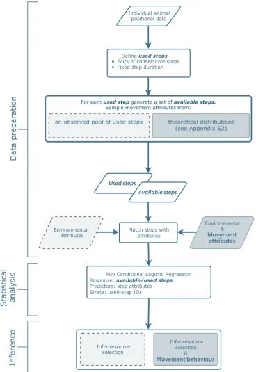
1. A resource selection function is a model of the likelihood that an available spatial unit will be used by an ani-mal, given its resource value. But how do we appropriately define availability? Step selection analysis deals with this problem at the scale of the observed positional data, by matching each ‘used step’ (connecting two consecu-tive observed positions of the animal) with a set of ‘available steps’ randomly sampled from a distribution of observed steps or their characteristics.

2. Here we present a simple extension to this approach, termed integrated step selection analysis (iSSA), which relaxes the implicit assumption that observed movement attributes (i.e. velocities and their temporal autocorrela-tions) are independent of resource selection. Instead, iSSA relies on simultaneously estimating movement and resource selection parameters, thus allowing simple likelihood-based inference of resource selection within a mechanistic movement model.

3. We provide theoretical underpinning of iSSA, as well as practical guidelines to its implementation. Using computer simulations, we evaluate the inferential and predictive capacity of iSSA compared to currently used methods.

4. Our work demonstrates the utility of iSSA as a general, flexible and user-friendly approach for both evaluat-ing a variety of ecological hypotheses, and predictevaluat-ing future ecological patterns.

Key-words: conditional logistic regression, dispersal, habitat selection, movement ecology, random walk, redistribution kernel, resource selection, step selection, telemetry, utilisation distribution

Introduction

Ecology is the scientific study of processes that determine the distribution and abundance of organisms in space and time (Elton 1927). Hence, asking how and why living beings change their spatial position through time is fundamental to ecological research (Nathan et al.2008). Animal movement links the behavioural ecology of individuals with population and community level processes (Lima & Zollner 1996). Its study is consequently vital for understanding basic ecological processes, as well as for applications in wildlife management and conservation.

Whether basic or applied, common to many empirical studies of animal movement is the aspiration to reliably pre-dict population density through space and time by modelling the spatiotemporal probability of animal occurrence, also known as the utilisation distribution (Keating & Cherry 2009). Despite much progress in statistical characterisation of animal movement and habitat associations, our ability to predict utilisation distributions is limited by our understand-ing of the underlyunderstand-ing behavioural processes. Indeed,

includ-ing explicit movement behaviours into spatial models of animal density has led to improved predictive performance (Moorcroft, Lewis & Crabtree 2006; Fordham et al. 2014). Deriving predictive space-use models based on the beha-vioural process underlying animal movement patterns is of particular importance when dealing with altered or novel landscapes that might differ substantially from the landscape used to inform the models.

Over the past three decades, a great deal of research has been dedicated to explaining and predicting spatial population dis-tribution patterns based on underlying habitat attributes (often termed resources). In that regard, much focus has been given to estimating resource selection functions (Manlyet al.2002)– phenomenological models of the relative probability that an available discrete spatial unit (e.g. an encountered patch or landscape pixel) will be used given its resource type/value (Lele

et al.2013). Indeed, its intuitive nature and ease of application has made resource selection analysis (RSA) the tool of choice for many wildlife scientists and managers seeking to use envi-ronmental information in conjunction with animal positional data (Boyce & McDonald 1999; McDonaldet al.2013; Boyce

et al.2015).

Whereas much progress has been gained in the application of RSAs to animal positional data, the problem of defining

*Correspondence author. E-mail: [email protected]

the appropriate spatial domain available to the animal remains as a major concern (Matthiopoulos 2003; Leleet al.

2013; McDonald et al. 2013; Northrup et al. 2013).

Weighted distribution approaches deal with this problem by modelling space-use as a function of a movement model and a selection function, but most weighted distribution models are challenging to implement (but see Johnson, Hooten & Kuhn 2013). Matched case–control logistic regressions (CLRs; also known as discrete-choice models) may be con-sidered a simplified alternative to the weighted distribution approach where each observed location is matched with a conditional availability set, limited to some predefined spatial and/or temporal range (Arthur et al. 1996; McCracken, Manly & Heyden 1998; Compton, Rhymer & McCollough 2002; Boyce et al. 2003; Baasch et al. 2010). A major strength of this approach is that maximum-likelihood esti-mates (MLEs) of the parameters can be efficiently obtained though commonly used statistical software (often relying on a Cox Proportional Hazard routine; e.g. functionclogit in R). One particular type of such conditional RSA is step selection analysis (SSA), where each ‘used step’ (connecting two consecutive observed positions of the animal) is coupled with a set of ‘available steps’ randomly sampled from the empirical distribution of observed steps or their characteris-tics (e.g. their length and direction; Fortinet al.2005; Duch-esne, Fortin & Courbin 2010; Thurfjell, Ciuti & Boyce 2014).

The definition of availability is challenging, however, even when using the SSA approach. The problem arises due to the sequential, rather than simultaneous, estimation of the move-ment and habitat-selection components of the process. Owing to this stepwise procedure, the resulting habitat-selection inference is conditional (on movement), whereas movement is assumed independent of habitat selection. In reality, the two are tightly linked, with habitat selection and availability affecting the animal’s movement patterns (Avgar et al.

2013b), and the animal’s movement capacity affecting its habitat-use patterns (Rhodeset al.2005; Avgaret al.2015). Failure to adequately account for the movement process may consequently lead to biased habitat-selection estimates (Fores-ter, Im & Rathouz 2009).

As we will show here, the benefits of adequately accounting for the movement process may extend beyond obtaining unbiased habitat-selection estimates. SSAs rely on a simple depiction of animal movement as a series of stochastic discrete steps, characterised by specific velocity and autocorrelation distributions. This same depiction underlies the mathematical modelling of animal movement as a discrete-time random walk (RW), including correlated and/or biased RW (Kareiva & Shigesada 1983; Turchin 1998; Codling, Plank & Benhamou 2008). Indeed, many SSA formulations correspond to a correlated RW process with local bias produced by resource selection (BCRW; Duchesne, Fortin & Rivest 2015). Apart from their com-patibility with the way we often observe animal movement (i.e. in continuous space and at discrete times), many RW can be well approximated by diffusion equations, allowing

a much sought shift from an individual-based Lagrangian perspective to population-level Eulerian models (Turchin 1991, 1998). SSAs are thus at an interface between statisti-cal (phenomenologistatisti-cal) RSAs and mathematistatisti-cal (mechanis-tic) RW models (Potts, Mokross & Lewis 2014b; Potts

et al. 2014a), models that form the backbone of much of the existing body of theory in the field of animal move-ment (Codling, Plank & Benhamou 2008; Benhamou 2014; Fagan & Calabrese 2014).

In this paper, we outline a CLR-based approach for simultaneous estimation of the movement and habitat-selec-tion components, an approach we nameintegrated step selec-tion analysis (iSSA; Fig. 1). The iSSA allows the effects of environmental variables on the movement and selection pro-cesses to be distinguished, thus providing a valuable tool for testing hypotheses (e.g. to test whether animals travel faster in certain times or through certain habitats), while resulting in an empirically parameterised mechanistic movement model (i.e. a mechanistic step selection model; Potts et al.

2014a), that can be used to translate individual-level observa-tions to population-level utilisation distribuobserva-tions across space and time (Pottset al.2014a; Potts, Mokross & Lewis 2014b; Appendix S1).

The iSSA is related to several recently published works integrating animal movement and resource selection. Both Forester, Im & Rathouz (2009) and Warton & Aarts (2013) demonstrated the inclusion of movement variables in an RSA and its marked effect on the resulting inference. Johnson, Hooten & Kuhn (2013) have shown that animal telemetry data can be viewed as a realisation of a non-homogenous space–time point process, and MLEs of this process can be obtained using a generalised linear model. These contributions focused on gaining unbiased resource selection inference while treating the movement process as nuisance that must be ‘controlled for’. Here, we seek expli-cit inference of this process. State-space models of animal movement (reviewed by Jonsen, Myers & Flemming 2003; and Patterson et al.2008) predict the future state (e.g. spa-tial position) of the animal given its current state (where an ‘observation model’ provides the probability of observ-ing these states), environmental covariates, and an explicit ‘process model’. Once parametrised, the process model can be used to generate space-use prediction, but parametrisa-tion is often technically demanding and computaparametrisa-tionally intensive (Patterson et al. 2008). More recently, Pottset al.

(2014a) demonstrated the use of a ‘mechanistic step selec-tion model’ to infer both the drivers and the steady-state distribution of animal space-use, but the model was framed around one specific functional form of the movement ker-nel, and parameter estimates were obtained using a cus-tom-made likelihood maximisation procedure. Lastly, Duchesne, Fortin & Rivest (2015) demonstrated that an SSA can be used to obtain unbiased estimates of the direc-tional persistence and bias of a BCRW, but did not address parametrisation of the step-length distribution.

movement process within an SSA, a complete habitat-depen-dent mechanistic movement model can be parametrised from telemetry data using a standard CLR routine. In the following, we provide a detailed description of the approach and evaluate its performance (compared with standard RSA and SSA) in correctly inferring the movement and habitat-selection processes underlying observed space-use patterns, and in pre-dicting the resulting UD.

Materials and methods

IN T E G R A T E D S T E P S E L E C T IO N A N AL Y S I S

In their work on the subject of accounting for movement in resource-selection analysis, Forester, Im & Rathouz (2009) demonstrated that including a distance function in SSA substantially reduces the bias in habitat-selection estimates. Mathematically, their argument is based

on the habitat-independent movement kernel (the function governing movement in the absence of resource selection, or across a homoge-neous landscape; Hjermann 2000; Rhodeset al.2005) belonging to the exponential family, so that it can be accounted for with the logistic formulation of the SSA likelihood function. Here we shall make the assumption that, in the absence of habitat selection, step lengths fol-low either an exponential, half-normal, gamma or log-normal distri-bution. Under this assumption, the statistical coefficients associated with step length, its square, its natural logarithm and/or the square of its natural logarithm (depending on the assumed distribution), when incorporated as covariates in a standard SSA, serve as statistical esti-mators of the parameters of the assumed step-length distribution (see Appendices S2 and S3 for details, and below for an example). Stan-dard model selection (e.g. likelihood ratio or AIC) then can be used to select the best-fit theoretical distribution (out of the four listed above). The iSSA approach moreover can be applied to infer directional per-sistence and external bias. Assuming that the angular deviations from preferred directions (either the previous heading, the target heading or both) are von Mises distributed (an analogue of the normal distribution on the circle), the cosine of these angular deviations can be included as covariates in an SSA to obtain MLEs of the corresponding von Mises concentration parameters (Duchesne, Fortin & Rivest 2015). Hence, MLEs of iSSA coefficients affiliated with directional deviations and step lengths are directly interpretable as the parameters of distributions governing the underlying BCRW.

We shall make the assumption here that animal space-use beha-viour is adequately captured by a separable model, involving the pro-duct of two kernels, a movement kernel and a habitat-selection kernel. Formally, we define a discrete-time movement kernel,Φ, which is pro-portional to the probability density of occurrence in any spatial posi-tion,x, at timet, in the absence of habitat selection. The determinants of_Φare as follows: the Euclidian distances betweenxand the preced-ing position, xt1 (the step length; lt= ||x–xt1||), the distances

betweenxt1andxt2(the previous step length;lt1= ||xt1–xt2||),

the associated step headings,atandat1(the directions of movement

fromxt1toxand fromxt2toxt1, respectively), and a vector of

spatial and/or temporal movement predictors at timetand/or at the vicinity ofxand/orxt1,Y(x,xt1,t) (e.g. terrain ruggedness,

migra-tory phase, snow depth, etc.). The effects of these step attributes onΦ are controlled by the associated coefficients vector,h. Note that the effects of spatial attributes here are assumed to operate through local biomechanical interactions between the animal and its immediate environment, interactions that determine the rate of displacement (i.e. kinesis), not where the animal ‘wants’ to be (i.e. taxis). Also note that the kernelΦcan be non-Markovian and accommodate various types of velocity autocorrelations (lack of independence between directions and/or lengths of consecutive steps), including correlated and biased random walks (if directional biases are knowna priori).

We further define the habitat-selection function,Ψ, which is propor-tional to the probability density of observing the animal in any spatial position,x, at timet, in the absence of movement constraints. The determinants of_Ψare the habitat attributes inxatt,H(x,t), and their corresponding selection coefficients,x. The normalised product ofΦ andΨyields the probability density of occurrence inxatt, which is:

f xð _tjxt1;xt2Þ ¼ U

lt;lt1;at;at1;Yðx;xt1;tÞ;h

½ W½H xð Þ;;t x Ð

XU½lt;lt1;at;at1;Yðx;xt1;tÞ;h W½H xð Þ;;t xdx:

eqn 1 Note that the same environmental variable (e.g. snow depth or ter-rain ruggedness) might be included in bothYandHand hence affect bothΦ[e.g. decreased speed in deep snow or across rugged terrain) and

Ψ(e.g. selection for snow-free or flat localities). Eqn 1 is equivalent to the formulation used (for example) by Rhodeset al.(2005, Eqn 1], Forester, Im & Rathouz (2009) and Johnson, Hooten & Kuhn (2013, Eqn 1) and is a generalised form of a redistribution kernel–a widely used mechanistic model of animal movement and habitat selection (see Discussion for recent examples).

The denominator in Eqn 1 is an integral over the entire spatial domain,Ω, serving as a normalisation factor to ensure the resulting probability density integrates to one. Whereas in most cases it would be impossible to solve this integral analytically, various forms of numerical (discrete-space) approximations can be used to fit redistri-bution kernel functions, such as Eqn 1, to data (see Avgar, Deardon & Fryxell 2013a and the Discussion). Here we focus on a simple like-lihood-based alternative to such numerical methods, one that can be implemented using common statistical software and is hence accessi-ble to most ecologists. Assuming an exponential form for both Φ andΨ, MLEs for the parameter vectorshandxcan be obtained using conditional logistic regression, where observed positions (cases) are matched with a sample of available positions (controls; Fig. 1 and Appendices S2–S4).

A HY P O T H E T I C A L E X A M P L E

Let us assume we have obtained a set ofTspatial positions, sampled at a unit temporal interval along an animal’s path, and that we also have maps of two (temporally stationary) spatial covariates,h(x) andy(x). We shall now assess the statistical support for the following proposi-tions (examples of the sort of hypotheses that could be tested):

A The animal is selecting high values ofh(x).

B At the observed temporal scale, and in the absence of variability inh

(x), the animal’s movement is directionally persistent (i.e. consecu-tive headings are posiconsecu-tively correlated), and the degree of this persis-tence varies withy(x) (e.g. the animal moves more directionally wherey(x) is lower). The resulting turn angles are von Mises dis-tributed with mean 0 (i.e. left and right turns are equally likely) and ay-dependent concentration parameter.

C At the observed temporal scale, and in the absence of variability inh

(x) andy(x), the animal’s movement is characterised by gamma dis-tributed step lengths, and the shape of this step-length distribution depends on the time of day (e.g. the animal moves faster during day-time).

Note that these propositions are contingent on the temporal gap between observed relocations (i.e. step duration), as well as on the spa-tial resolution of our covariate maps,h(x) andy(x). We thus explicitly acknowledge that our inference is scale dependent.

We start by sampling, for each (but the first two) of the observed points along a path (xt,t=3, 4,. . .,T), a set ofscontrol points

(avail-able spatial positions at timet;x0_t;i,i=1, 2,. . .,s), where the probability of obtaining a sample at some distance,l0_t;i, from the previous observed point (l0_t;i¼ kx_t0_;ixt1k) is given by the gamma PDF:

g l0_t;ijb1;b2

¼ 1 Cðb1Þb2b1

l0_t;ib11_e

l0 t;i

b_{2 eqn 2}

Here,b1andb2are initial estimates of the gamma shape and scale

habitat-indepen-dent shape and scale (Appendices S2–S3). Note that these control sets also could be sampled randomly within some finite spatial domain (e.g. within the maximal observed displacement distance; Appendices S2 and S4). Distance weighted sampling is expected to increase inferential efficiency, resulting in a smaller standard error for a givensvalue, but is not a necessity (Forester, Im & Rathouz 2009). In general, any increase inTand/orswill result in better approximation of the used and/or availability distributions (respectively), and hence better inference (together with larger computational costs).

Once sampled, control (available) points,x0_t;i, are assigned a value of 0, whereas the observed (used or case) points,xt, are assigned a value of

1. The resulting binomial response variable can now be statistically modelled using conditional (case–control) logistic regression, as the likelihood of the observed data is exactly proportional to (Gail, Lubin & Rubinstein 1981; Forester, Im & Rathouz 2009; Duchesne, Fortin & Rivest 2015):

wherea0_t;iis the direction of movement fromxt1tox0t;i, andDtis an

indicator variable having the value 1 whentis daytime and 0 otherwise. Note that the summation in the denominator starts ats=0 (rather than 1) to indicate that the used step is included in the availability set (x0_t;i¼0¼xt). Also note that it is the inclusion of turn angles that

neces-sitates the exclusion of the first two positions (xt= 1andxt= 2); if no

velocity autocorrelation is modelled, only the first position is excluded. Lastly, note that this formulation implies that the degree of directional persistence is affected by the value ofyat the onset of the step only; in the next section, we provide an example of modelling habitat effects on movement along the step.

Equation 3 is a discrete-choice approximation of Eqn 1 (specifi-cally tailored according to propositions A–C), and we provide its full derivation in Appendix S3. In summary,b3is the

habitat-selec-tion coefficient (corresponding to proposihabitat-selec-tion A and estimating the only component of the parameter vector x in Eqn 1), b4 and b5

are the basal (habitat-independent) and y-dependent directional persistence coefficients (corresponding to proposition B and esti-mating two components of the parameter vector hin Eqn 1), and

b6, b7andb8 are the modifiers of the step-length shape and scale

coefficients (corresponding to proposition C and estimating the remaining components of the parameter vector h). Once maxi-mum-likelihood estimates are obtained, the shape and scale param-eters of the basal step-length distribution can be calculated (Appendix S3), where the shape is given by: [(b1+b7)+b8.Dt],

and the scale is given by: [1/(b21–b6)]. Similarly,b4can be shown

to be an unbiased estimator of the concentration parameter of the (habitat-independent) von Mises turn angles distribution (Duch-esne, Fortin & Rivest 2015).

Including movement attributes as covariates in SSA, which we termed here iSSA, thus allows simple likelihood-based estimation of explicit ecological hypotheses within a framework of a mechanistic habitat-mediated movement model. Such hypotheses might include, in addition to those mentioned thus far, long- and short-term target prioritisation (Duchesne, Fortin & Rivest 2015), barrier crossing and avoidance behaviour (Beyeret al.2015), and interactions with conspecifics and intraspecifics (Latombe, Fortin & Parrott 2014; Potts, Mokross & Lewis 2014b; Pottset al.2014a). In fact, many of the facets of the generic approach developed by Langrock et al.

(2012) can be included in an iSSA with the MLEs obtained using standard statistical packages. An iSSA thus holds promise as a user-friendly yet versatile approach in the movement ecologist’s toolbox. In Appendix S4, we provide practical guidelines for the application of iSSA. In the next sections, we explore the utility of this approach using computer simulations.

S IM U L A T IO N S

Testing the inferential and predictive capacities of any statistical space-use model is challenging because we are often ignorant of the true process giving rise to the observed patterns, as well as of the true distri-bution of space-use from which these patterns are sampled (Avgar, Deardon & Fryxell 2013a; Van Moorteret al.2013). To deal with this challenge, we employ here a simple process-based movement

simulation framework. We provide full details of the simulation procedure and its statistical analysis in Appendix S5.

Fine-scale space-use dynamics were simulated using stochastic ‘stepping-stone’ movement across a hexagonal grid of cells. Each cell,x, is characterised by habitat quality,h(x) with spatial autocor-relation set by an autocorautocor-relation range parameter,q(=0, 1, 5, 10 and 50). For each q value, 1000 trajectories were simulated and then rarefied (by retaining every 100th position). Each of these rar-efied trajectories was then separately analysed using RSA and 10 different (i)SSA formulations, including one or more of the follow-ing covariates (Table 1): habitat values at the end of each step,h

(xt), the average habitat value along each step,h(xt1,xt), the step

length, lt(=||xt1–xt||), its natural-log transformation, ln(lt), and

the statistical interactions between lt, ln(lt) and h(xt1,xt). Models

that included onlyh(xt) and/orh(xt1,xt) correspond to traditionally

used SSA (relying on empirical movement distributions with no movement attribute included as covariates; models a, b and c in Table 1), whereas models that additionally includedltand ln(lt)

cor-respond to iSSA. The predictive capacity of the models was esti-mated based on the agreement between their predicted utilisation distributions (UD) and the ‘true’ UD, generated by the true under-lying movement process. We refer the reader to Appendix S5 for further details.

A separate simulation study was conducted to evaluate the identifia-bility and estimaidentifia-bility of the iSSA parameters as function of sample size and habitat-selection strength (Appendix S6).

Results

P A R A M E T E R I S A T I O N

All models converged in a timely manner and the convergence time for the most complex model (model jin Table 1) was approximately 1 CPU sec. Of the 10 (i)SSA formulations speci-fied in Table 1, AIC ranking indicated support for only four (d,f,handj), all of which include the habitat value at the step’s endpoint (with coefficientb3) and the step length and its natu-ral logarithm (with coefficientsb5andb6) as covariates. Hence,

YT

t¼3

exp½b3hðxtÞ þ ½b4þb5yðxt1Þ cosðat1atÞ þb6ltþ ðb7þb8DtÞlnðltÞ

Ps

i¼0exp½b3hðx0t;iÞ þ ½b4þb5yðxt1Þcosðat1a0t;iÞ þb6l0t;iþ ðb7þb8DtÞlnðl0t;iÞ

iSSAs better explain our simulated data than traditionally used SSAs (excluding step length as a covariate), but only as long as an endpoint effect (i.e. selection for/against the habitat value at the end of the step) is included. In fact, models that excluded the habitat value at the step’s endpoint (modelsb,e,gandi) had AIC scores that were typically two orders of magnitude larger than those including it. In comparison to RSA, iSSA formulations had unequivocal AIC support at low habitat spa-tial autocorrelation levels, but only parspa-tial support at high autocorrelation levels (Table 1).

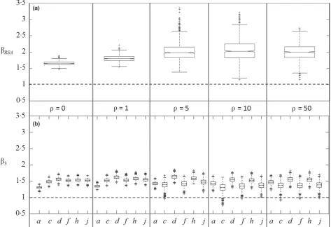
Estimated habitat-selection strengths, as indicated by our RSA and SSA coefficient estimates (bRSAandb3,respectively), were appreciably larger than the true habitat-selection strength (x=1), and more so for RSA estimates than for SSA (Fig. 2). Note that this in itself does not mean these estimates are ‘bi-ased’ but rather reflects the inherent difference between the intensity of the true process and that of the emerging pattern, at the scale of observation (see further discussion below). These estimates showed little sensitivity to the level of habitat spatial autocorrelation, although a substantial increase in variance is observed in the RSA case (Fig. 2a). As found before by Fores-ter, Im & Rathouz (2009), the strength of SSA-inferred habitat selection is larger when step lengths are included as a covariate in the analysis (iSSA), but this effect is fairly weak and dimin-ishes as the habitat’s spatial autocorrelation increases (Fig. 2b).

Overall, SSA-inferred habitat selections were substantially less variable than RSA-based estimates and showed little sensi-tivity to the inclusion or exclusion of other covariates in the model fit (Fig. 2). This is not the case, however, for the effect of the mean habitat value along the step (b4), which varied sub-stantially with both the level of habitat spatial autocorrelation and the inclusion of an endpoint effect (b3). Whereb3was not included in the model fit (modelsb,eandiin Table 1),b4 increased withq, whereas whereb3was included (modelsc,f

andj),b4was closer to zero (Fig. 3). Interestingly, when only the habitat at the end of the step and the habitat along the step were included in the model (i.e. modelc; a commonly used SSA formulation), and at lowqvalues (=0, 1),b4was negative, indicating ‘selection against’ high-quality steps. In fact, this reflects the low probability of observing a ‘used’ step that tra-verses high-quality habitat but does not end there.

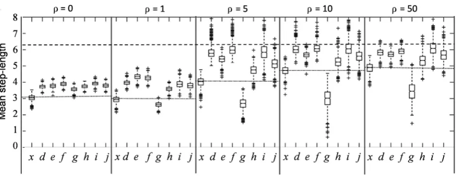
As explained above (and in Appendices S2 and S3), iSSA coefficients affiliated with the step length (b5) and its natural logarithm (b6), when combined with the estimated shape and scale values of the observed step-length distribution (b1andb2; on which sampling was conditioned; Appendices S3 and S5), could be used to infer the shape and scale of the ‘habitat-inde-pendent’ step-length distribution [i.e. assumingh(xt,xt+1)=0]. Under most imaginable scenarios, we would expect this basal movement kernel to be wider (i.e. with larger mean) than the observed one, as animals tend to linger in preferred habitats and hence display more restricted movements compared to the basal expectation. Indeed, the mean of these inferred distribu-tions (the product of their shape and scale: _ðð_bb11þb6Þ

2 b5Þ

) corre-sponds exactly to the observed mean, as long as no other covariates are included in the analysis (model x in Fig. 4). Once other covariates are included in the model (and hence habitat selection is at least partially accounted for), inferred mean step-length values were significantly higher from the observed values, showed little sensitivity to model structure, but increased withq(as do the observed mean step lengths). One exception is modelg, which strongly underestimated the mean step length at moderate-high q values as it does not include any main habitat effects.

Even at highqvalues, inferred mean step length slightly but consistently underestimates the true habitat-independent step-length distribution (calculated by simulating the process based on Eqn S51 withx=0; Fig. 4). This bias is a result of an iSSA’s limited capacity to account for the full movement

Table 1.The 11 different models fitted here and their relative performance ranking at five different levels of habitat spatial autocorrelation (with 1000 realisations at each level). To enable AIC comparison, RSA’s were run with only those positions included in the SSA (i.e. excluding the first position)

Model

Covariates % Scord as best (based on AIC)

R(xt) R(xt,xt1) lt ln (lt)

R(xt,xt1)

lt

R(xt,xt1)

ln (lt) q=0 q=1 q=5 q=10 q=50

RSA bRSA 0 0 0 0 0 0 0 203 457 447

SSA

a b3 0 0 0 0 0 0 0 0 0 0

b 0 b4 0 0 0 0 0 0 0 0 0

c b3 b4 0 0 0 0 0 0 0 0 0

iSSA

d b3 0 b5 b6 0 0 0 0 0 11 11

e 0 b4 b5 b6 0 0 0 0 0 0 0

f b3 b4 b5 b6 0 0 104 44 139 240 284

g 0 0 b5 b6 b7 b8 0 0 0 0 0

h b3 0 b5 b6 b7 b8 662 283 107 5 23

i 0 b4 b5 b6 b7 b8 0 0 0 0 0

j b3 b4 b5 b6 b7 b8 234 673 551 233 235

process as it unfolds in between observations. The animal does not actually travel along the straight lines that we term ‘steps’ and, even if it would, the mean habitat value along the step does not exactly correspond to its probability to travel farther. As long as the scale of the observation is coarser than the scale

of the underlying movement process, the animal’s true move-ment capacity is never fully manifested in the observed reloca-tion pattern and is thus always underestimated. Note, however, that this bias is negligibly small where the spatial autocorrelation of habitats is high (q>1; Fig. 4).

(a)

(b)

Fig. 2. Statistically inferred habitat-selection coefficient estimates for RSA (a) and SSA (b; letters along thex-axis refer to the SSA formulations listed in Table 1), for five levels of habitat spatial autocorrelation,_q. Each box-and-whiskers is based on 1000 independent estimates, where the cen-tral mark is the median, the edges of the box are the 25th and 75th percentiles, the whiskers extend to the most extreme data points not considered outliers (i.e. within approximately 99% coverage if the data are normally distributed), and outliers are plotted individually. Horizontal dashed lines represent the true habitat-selection intensity,x=1. See Appendix S5 for further details.

Finally, despite apparent support for iSSA formulations including interaction between the step length and habitat qual-ity along the step (Table 1; modelshandj), the estimated val-ues of the interaction coefficients,b7andb8, mostly overlapped zero (Appendix S7). Generally speaking, the mean habitat value along the step has a weak negative effect on both the shape (throughb8) and the scale (through its inverse relation-ship withb7) of the step-length distribution–long steps are less likely through high-quality habitats.

P R E D ICT IV E C A P A C IT IE S

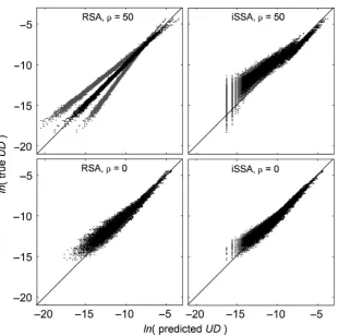
At approximate steady state, RSA-based UD predictions are slightly more accurate and precise than SSA-based predictions (Fig. 5 and Appendix Table S8). The RSA’s predictive capac-ity increases withq(while its precision dramatically decreases), whereas the opposite is true for SSA predictions, where the minimum KLD value (Kullback-Leibler Divergence; see Appendix S5) is reached whenq=0 (Appendix Table S8).

KLDvalues coarsely mirror the AIC ranking of the different SSA formulations in distinguishing those that include an end-point effect (b3), but the best performing formulations based onKLDare simpler than the ones selected based on AIC (Tables 1 and S8). That said, all iSSA formulations including an endpoint effect performed well overall, withGKLDscores (a measure of goodness of fit; Appendix S5) ranging from~084 (modelfwhenq=50) to~098 (modeldwhenq=0). For ref-erence, theGKLD scores for RSA-based predictions ranged from~098 (q=0) to~099 (q=50).

To test the sensitivity of the models’ predictions to the sampling scale (see Appendix S9 for relatingqto the sam-pling scale), we generated predicted UDs, both SSA-based and RSA-based, across a highly autocorrelated landscape (q=50) using parameter estimates obtained from samples of a random landscape (q=0), and vice versa. RSA-based

predictions were robust to these scale mismatches, withGKLD scores of ~098 and ~096, for the q=50 landscape (with parameter estimates based on q=0 data) and the q =0 landscape (with parameter estimates based onq=50 data), respectively. Similarly, all step selection models including an endpoint effect performed well, with GKLD scores ranging from~094 (modelf) to~098 (modelh) for theq=0 land-scape (with parameter estimates based onq=50 data), and

GKLDscores ranging from~083 (modelj) to~097 (modela) for theq =50 landscape (with parameter estimates based on

q=0 data). Overall, iSSA-based predictive capacity remained mostly unaltered by mismatches between the data’s landscape structure and the structure of the landscape on which projections are made.

As can be expected, step selection models predict transient UDs better than the inherently stationary RSA (except when

q=50; Appendix Table S8). In comparison with steady-state predictions, complex iSSA-based predictions perform better than simpler ones (Appendix Table S8). As for the steady-state predictions, all iSSA formulations including an endpoint effect performed well in predicting transient UDs, withGKLDscores ranging from~89% (modelhwhenq=0) to~098 (modeld

whenq=1).GKLDscores for RSA-based predictions showed substantial sensitivity to the level of spatial autocorrelation, ranging from~069 (q=0) to~097 (q=50).

IS S A ID E N T IF IA B IL I T Y A N D E S T IMA B I L IT Y

Results are presented in detail in Appendix S6. In short, our analysis revealed that, under the test scenario, all iSSA parameters are fully identifiable, that estimates are unbiased in relation to the true values of the kernel generating func-tions, and that an increase in sample size beyond ~400 observed positions does not seem to substantially enhance precision (and hence estimability). That said, our results also

indicate that inferential accuracy of movement related param-eters may be highly variable, leading to compromised preci-sion (with up to 1000% departure from the true value; Appendix S6) even at a fairly large sample size. This may be particularly true given the inherent trade-off between sam-pling extent and frequency (Fieberg 2007). Estimability of cer-tain parameters, under cercer-tain scenarios, may thus be weak and must be evaluated on a case-by-case basis.

Discussion

The ideas, simulations and results presented above are aimed at providing a comprehensive assessment of using integrated step selection analysis, iSSA, with emphasis on its predictive capacity. The iSSA allows simultaneous inference of habitat-dependent movement and habitat selection and is hence a powerful tool for both evaluating ecological hypotheses and predicting ecological patterns. We have shown that iSSA-based habitat-selection inference is relatively insensitive to model structure and landscape configuration, and that iSSA-based UD predictions perform well across different temporal and spatial scales (we discuss the connection between the temporal resolution of the data and the habitat spatial auto-correlation in Appendix S9). On the other hand, our results indicate that movement and habitat selection may not be com-pletely separable once observations are collected at a coarser temporal resolution than the underlying behavioural process. Consequently, stationary RSA-based predictions, whereas much simpler to obtain, provide slight but consistent better fit

to the true UD when the time-scale is long (and hence approaches the steady-state limit).

Two caveats are in place here. First, in our analysis the defi-nition of the availability set for the RSA was exact (i.e. the entire domain), a situation that seldom occurs in empirical studies where availability is unknown. This is not the case for iSSA where the availability set always can be adequately defined (but is conditional on the temporal resolution of the positional data). Secondly, the high variability characterising the RSA coefficient estimates, and its resulting predictions (Figs 2 and 5) indicate substantial risk of erroneous inference. This may be particularly true when sample size is smaller than the relatively large sample used here, resulting in data that are not adequate unbiased samples of the steady-state UD, which is likely the case in most empirical studies. The more mechanis-tic nature of the iSSA makes it less sensitive to stochasmechanis-tic differ-ences between specific realisations of the space-use process (e.g. due to differences in landscape configuration) and thus leads to more precise inference. Hence, even if the sole objec-tive of a given study is to predict the long-term (steady-state) utilisation distribution, the more complicated iSSA-based pre-dictions might be more reliable than those based on RSA. Moreover, in many real-world ecological scenarios, a steady state is never reached, and consequently, the static RSA-based approach is less appropriate than the dynamical iSSA. We thus conclude that iSSA should be the method of choice whenever: (i) RSA availability cannot be properly defined, (ii) predicting across a landscape different from the landscape used for parametrisation, (iii) the data used for parametrisation are not

an adequate sample of the true steady-state UD or (iv) predict-ing transient space-use dynamics.

Many movement and selection processes could be consid-ered plausible, and the particular details of the mechanistic model used to simulate space-use data might substantially alter our conclusions. Our aim here was to use the simplest, and hence most general, mechanistic process imaginable, leading us to choose a stepping-stone movement process as our pat-tern-generating process. Interestingly, this simple process, gov-erned by only two parameters (Eqn S5.1), gave rise to complex patterns once rarefied. In particular, the emerging step-length distributions fit remarkably well with a gamma distribution, with shape and scale that reflect the underlying landscape structure. Note that this is a purely phenomenological descrip-tion of the movement kernel, as the true underlying process had a fixed, habitat-independent movement parameter (Appendix S5). Ideally, a truly mechanistic approach will involve maximising the likelihood over all possible paths the animal might have taken between two observed locations, and hence allowing inference of the true underlying process (Mat-thiopoulos 2003). In most cases, however, this approach is for-biddingly computationally expensive. We showed that the approximation based on samples of straight-line movements between observed positions, which is the underlying assump-tion of any SSA, performs well over a range of condiassump-tions. An iSSA thus provides a reasonable compromise between compu-tationally intensive mechanistic models and the purely phe-nomenological RSA.

According to Barnett & Moorcroft (2008), the steady-state UD should scale linearly with the underlying habitat-selection

function Ψ (Eqn 1) when informed movement capacity

exceeds the scale of spatial variation inΨ, but should scale with the square ofΨif informed movement capacity is much shorter than the scale of habitat variation. In the particular case of the exponential habitat-selection function used here (Eqn S5.1), we would thus expect the following loglinear relationship:ln

[UD(x)]=a+b∙x∙h(x), where ais a scaling parameter [the utilisation probability where h(x)=0], and b (1≤b≤2) is some increasing function of the habitat spatial autocorrelation,

q. Our results, emerging from a very different model than the continuous-space continuous-time analytical approximation of Barnett & Moorcroft (2008), corroborate this expectation. The slope of the loglinear regression model described above increases fromb 14 tob 2 asqincreases from 0 to 50 (Appendix S10). RSA-based coefficient estimates,bRSA, clo-sely mirror this pattern, increasing from ~16 to ~2 as q increases (Fig. 2a). Hence, as can be expected from a phe-nomenological model, RSA-based inference reflects the steady-state UD rather than the underlying habitat-selection process.

Recent years have seen a proliferation of sophisticated modelling approaches aimed at mechanistically capturing animal space-use behaviours. Many of these models share the theoretical underpinning of iSSA (as formulated in Eqn 1), relying on a depiction of animal space-use as emerging from the product of a resource-selection process and a selection-independent movement kernel (e.g. Rhodes

et al. 2005; Getz & Saltz 2008; Avgar, Deardon & Fryxell 2013a; Potts et al. 2014a; Beyer et al. 2015). Unlike the iSSA, however, fitting these kernel-based models to empiri-cal data relies on complex, and often specifiempiri-cally tailored likelihood maximisation algorithms (namely discrete-space approximations of the integral in Eqn 1). The statistical machinery used in iSSA, based on obtaining a small set of random samples from an inclusive availability domain, is accessible to most ecologists because it relies on software that is already used (Thurfjell, Ciuti & Boyce 2014). Through the addition of appropriate covariates and interac-tion terms, iSSA can moreover address many of the ques-tions that were the focus of other kernel-based approaches, such as home-range behaviour (Rhodes et al. 2005), mem-ory-use (Avgar, Deardon & Fryxell 2013a; Merkle, Fortin & Morales 2014; Avgaret al.2015; Schl€agel & Lewis 2015), habitat-dependent habitat selection (Potts et al. 2014a) and barrier effects (Beyeret al.2015). Hence, iSSA allows ecolo-gists to tackle complicated questions using simple tools.

To conclude, our work complements several recent contri-butions advocating the use of movement covariates within step selection analysis (Forester, Im & Rathouz 2009; Johnson, Hooten & Kuhn 2013; Warton & Aarts 2013; Duchesne, For-tin & Rivest 2015). We believe a convincing body of theoretical evidence now indicates the suitability of integrated step selec-tion analysis as a general, flexible and user-friendly approach for both evaluating ecological hypotheses and predicting future ecological patterns. Our work highlights the importance of including endpoint effects in the analysis together with some caveats regarding the interpretation of SSA results, specifically when dealing with the effects of the habitat along the step. We also recommend careful consideration of parameter estimabil-ity, particularly with regard to the movement components of the model, which may be prone to strong cross-correlations (as discussed in Appendix S6). Based on our current experience in applying iSSA to empirical data (T. Avgar, work in progress) we have provided practical guidelines in Appendix S4. Addi-tional theoretical work is needed to investigate the effects of the underlying movement process on iSSA performance, as well as to come up with computationally efficient iSSA-based simulations to enable rapid generation of predicted utilisation distribution (as discussed in Appendix S1). Most importantly, the utility of iSSA must now be evaluated by applying it to real data sets, and using it to solve real ecological problems.

Acknowledgements

TA gratefully acknowledges supported by the Killam and Banting Postdoctoral Fellowships. MAL gratefully acknowledges NSERC Discovery and Accelerator Grants and a Canada Research Chair. MSB thanks NSERC and the Alberta Conservation Association for funding. The authors thank L. Broitman for designing Fig. 1 and C. Prokopenko for helpful editorial comments, and Dr. Geert Aarts, Dr. John Fieberg and an anonymous reviewer, for their instructive comments and suggestions.

Data accessibility

References

Arthur, S.M., Manly, B.F.J., Mcdonald, L.L. & Garner, G.W. (1996) Assessing habitat selection when availability changes.Ecology,77, 215–227.

Avgar, T., Deardon, R. & Fryxell, J.M. (2013a) An empirically parameterized individual based model of animal movement, perception and memory. Ecolog-ical Modelling,251, 158–172.

Avgar, T., Mosser, A., Brown, G.S. & Fryxell, J.M. (2013b) Environmental and individual drivers of animal movement patterns across a wide geographical gradient.Journal of Animal Ecology,82, 96–106.

Avgar, T., Baker, J.A., Brown, G.S., Hagens, J., Kittle, A.M., Mallon, E.E.et al. (2015) Space-use behaviour of woodland caribou based on a cognitive move-ment model.Journal of Animal Ecology,84, 1059–1070.

Baasch, D.M., Tyre, A.J., Millspaugh, J.J., Hygnstrom, S.E. & Vercauteren, K.C. (2010) An evaluation of three statistical methods used to model resource selection.Ecological Modelling,221, 565–574.

Barnett, A.H. & Moorcroft, P.R. (2008) Analytic steady-state space use patterns and rapid computations in mechanistic home range analysis.Journal of Mathe-matical Biology,57, 139–159.

Benhamou, S. (2014) Of scales and stationarity in animal movements.Ecology Letters,17, 261–272.

Beyer, H.L., Gurarie, E., Borger, L., Panzacchi, M., Basille, M., Herfindal, I., Van Moorter, B., Lele, S. & Matthiopoulos, J. (2015) ‘You shall not pass!’: quantifying barrier permeability and proximity avoidance by animals.Journal of Animal Ecology,85, 43–53.

Boyce, M.S. & McDonald, L.L. (1999) Relating populations to habitats using resource selection functions.Trends in Ecology & Evolution,14, 268–272. Boyce, M.S., Mao, J.S., Merrill, E.H., Fortin, D., Turner, M.G., Fryxell, J.M. &

Turchin, P. (2003) Scale and heterogeneity in habitat selection by elk in Yel-lowstone National Park.Ecoscience,14, 421431.

Boyce, M.S., Johnson, C.J., Merrill, E.H., Nielsen, S.E., Solberg, E.J. & Van Moorter, B. (2015) Can habitat selection predict abundance?Journal of Animal Ecology,85, 11–20.

Codling, E.A., Plank, M.J. & Benhamou, S. (2008) Random walk models in biol-ogy.Journal of the Royal Society Interface,5, 813–834.

Compton, B., Rhymer, J. & McCollough, M. (2002) Habitat selection by wood turtles (Clemmys insculpta): an application of paired logistic regression. Ecol-ogy,83, 833–843.

Duchesne, T., Fortin, D. & Courbin, N. (2010) Mixed conditional logistic regres-sion for habitat selection studies.Journal of Animal Ecology,79, 548–555. Duchesne, T., Fortin, D. & Rivest, L. (2015) Equivalence between step selection

functions and biased correlated random walks for statistical inference on ani-mal movement.PLoS ONE,10, e0122947.

Elton, C.S. (1927, 2001)Animal ecology. University of Chicago Press, Chicago, IL, USA.

Fagan, W. & Calabrese, J. (2014) The correlated random walk and the rise of movement ecology.Bulletin of the Ecological Society of America,95, 204–206. Fieberg, J. (2007) Kernel density estimators of home range: smoothing and the

autocorrelation red herring.Ecology,88, 1059–1066.

Fordham, D.A., Shoemaker, K.T., Schumaker, N.H., Akcßakaya, H.R., Clisby, N. & Brook, B.W. (2014) How interactions between animal movement and landscape processes modify local range dynamics and extinction risk.Biology Letters,10, 20140198.

Forester, J.D., Im, H.K. & Rathouz, P.J. (2009) Accounting for animal move-ment in estimation of resource selection functions: sampling and data analysis. Ecology,90, 3554–3565.

Fortin, D., Beyer, H.L., Boyce, M.S., Smith, D.W., Duchesne, T. & Mao, J.S. (2005) Wolves influence elk movements: behavior shapes a trophic cascade in Yellowstone National Park.Ecology,86, 1320–1330.

Gail, M.H., Lubin, J.H. & Rubinstein, L.V. (1981) Likelihood calculations for matched case-control studies and survival studies with tied death times. Biome-trika,68, 703–707.

Getz, W.M. & Saltz, D. (2008) A framework for generating and analyzing move-ment paths on ecological landscapes.Proceedings of the National Academy of Sciences of the United States of America,105, 19066–19071.

Hjermann, D.Ø. (2000) Analyzing habitat selection in animals without well-defined home ranges.Ecology,81, 1462–1468.

Johnson, D.S., Hooten, M.B. & Kuhn, C.E. (2013) Estimating animal resource selection from telemetry data using point process models.Journal of Animal Ecology,82, 1155–1164.

Jonsen, I.D., Myers, R.A. & Flemming, J.M. (2003) Meta-analysis of animal movement using state-space models.Ecology,84, 3055–3063.

Kareiva, P.M. & Shigesada, N. (1983) Analyzing insect movement as a correlated random-walk.Oecologia,56, 234–238.

Keating, K.A. & Cherry, S. (2009) Modeling utilization distributions in space and time.Ecology,90, 1971–1980.

Langrock, R., King, R., Matthiopoulos, J., Thomas, L., Fortin, D. & Morales, J.M. (2012) Flexible and practical modeling of animal telemetry data: hidden Markov models and extensions.Ecology, 93, 2336–2342.

Latombe, G., Fortin, D. & Parrott, L. (2014) Spatio-temporal dynamics in the response of woodland caribou and moose to the passage of grey wolf.Journal of Animal Ecology,83, 185–198.

Lele, S.R., Merrill, E.H., Keim, J. & Boyce, M.S. (2013) Selection, use, choice and occupancy: clarifying concepts in resource selection studies.Journal of Animal Ecology,82, 1183–1191.

Lima, S.L. & Zollner, P.A. (1996) Towards a behavioral ecology of ecological landscapes.Trends in Ecology & Evolution,11, 131–135.

Manly, B.F.J., McDonald, L.L., Thomas, D.L., McDonald, T.L. & Erick-son, W.P. (2002)Resource selection by animals: statistical design and anal-ysis for field studies, 2nd edn. Kluwer Academic Publishers, Dordrecht, Netherlands.

Matthiopoulos, J. (2003) The use of space by animals as a function of accessibility and preference.Ecological Modelling,159, 239–268.

McCracken, M.L., Manly, B.F.J. & Heyden, M.V. (1998) The use of discrete-choice models for evaluating resource selection.Journal of Agricultural, Biolog-ical, and Environmental Statistics,3, 268–279.

McDonald, L., Manly, B., Huettmann, F. & Thogmartin, W. (2013) Location-only and use-availability data: analysis methods converge (G. Hays, Ed.). Jour-nal of Animal Ecology,82, 1120–1124.

Merkle, J., Fortin, D. & Morales, J. (2014) A memory-based foraging tactic reveals an adaptive mechanism for restricted space use.Ecology Letters,17, 924–931.

Moorcroft, P.R., Lewis, M.A. & Crabtree, R.L. (2006) Mechanistic home range models capture spatial patterns and dynamics of coyote territo-ries in Yellowstone. Proceedings of the Royal Society B, 273, 1651– 1659.

Nathan, R., Getz, W.M., Revilla, E., Holyoak, M., Kadmon, R., Saltz, D. & Smouse, P.E. (2008) A movement ecology paradigm for unifying organismal movement research.Proceedings of the National Academy of Sciences of the United States of America,105, 19052–19059.

Northrup, J., Hooten, M., Anderson, C.R. Jr & Wittemyer, G. (2013) Practical guidance on characterizing availability in resource selection functions under a use-availability design.Ecology,94, 1456–1463.

Patterson, T.A., Thomas, L., Wilcox, C., Ovaskainen, O. & Matthiopoulos, J. (2008) State-space models of individual animal movement.Trends in Ecology & Evolution,23, 87–94.

Potts, J.R., Mokross, K. & Lewis, M.A. (2014b) A unifying framework for quan-tifying the nature of animal interactions.Journal of the Royal Society Interface,

11, 20140333.

Potts, J.R., Bastille-Rousseau, G., Murray, D.L., Schaefer, J.A. & Lewis, M.A. (2014a) Predicting local and non-local effects of resources on animal space use using a mechanistic step-selection model.Methods in Ecology and Evolution,5, 253–262.

Rhodes, J., McAlpine, C., Lunney, D. & Possingham, H. (2005) A spatially expli-cit habitat selection model incorporating home range behavior.Ecology,86, 1199–1205.

Schl€agel, U. & Lewis, M. (2015) Detecting effects of spatial memory and dynamic information on animal movement decisions.Methods in Ecology and Evolu-tion,11, 1236–1246.

Thurfjell, H., Ciuti, S. & Boyce, M.S. (2014) Applications of step-selection functions in ecology and conservation.Movement Ecology,2, 4. Turchin, P. (1991) Translating foraging movements in heterogeneous

envi-ronments into the spatial distribution of foragers. Ecology, 72, 1253–

1266.

Turchin, P. (1998) Quantitative analysis of movement. Sinauer, Sunderland, MA.

Van Moorter, B., Visscher, D., Herfindal, I., Basille, M. & Mysterud, A. (2013) Inferring behavioural mechanisms in habitat selection studies–getting the null-hypothesis right for functional and familiarity responses.Ecography,36, 323–330.

Warton, D. & Aarts, G. (2013) Advancing our thinking in presence-only and used-available analysis.Journal of Animal Ecology,82, 1125–1134.

Supporting Information

Additional Supporting Information may be found in the online version of this article.

Appendix S1.From step selection to utilisation distribution.

Appendix S2.Inferring step-length distributions.

Appendix S3.Deriving an iSSA likelihood function.

Appendix S4.iSSA practical user guide.

Appendix S5.Simulation experiments.

Appendix S6.Evaluating the iSSA parameter identifiability and estima-bility.

Appendix S7._b7 and_b8.

Appendix S8.Predictive performance.

Appendix S9.Interpretingq.

Appendix S10.Habitat selection and utilisation distribution.