Finite Element Analysis of the Material’s Area Affected during a Micro Thermal Analysis Applied to Homogeneous Materials

doi:10.4236/jsemat.2011.11001 Published Online April 2011 (http://www.SciRP.org/journal/jsemat)

Finite Element Analys

i

s of the Material’s Area

Affected during a Micro Thermal Analysis Applied

to Homogeneous Materials

Yoann Joliff*, Lénaïk Belec, Jean-François Chailan

MAPIEM, EA 4323, Institut des Sciences de l’Ingénieur de Toulon et du Var, Cedex, France Email: [email protected]

Received February 2nd_{, 2011; revised March 15}th_{, 2011; accepted March 20}th_{, 2011.}

ABSTRACT

Micro-thermal analysis (µ-TA), with a miniaturized thermo-resistive probe, allows topographic and thermal imaging of surfaces to be carried out and permits localized thermal analysis of materials. In order to estimate the effective volume of material thermally affected during this localized measurement, simulations, using finite element method were used. Several parameters and conditions were considered. So, thermal conductivity was found to be the driving physical pa-rameter in thermal exchanges. Indeed, the evolution of the heat affected zone (HAZ) versus thermal conductivity can well be described by a linear interpolation. Therefore it is possible to estimate the HAZ before experimental measure-ments. This result is an important progress especially for accurate interphase characterization in heterogeneous mate-rials.

Keywords: Micro-Thermal Analysis, Localized Thermal Analysis, Heat Affected Zone, Thermal Conductivity, Finite

Element Method

1. Introduction

Micro thermal analysis is a characterization technique of thermal and mechanical behaviours of materials at sub-microscopic scale [1]. This technique is therefore dedi-cated to numerous application domains dealing with low scale characterizations such as distinguishing different constituents of a heterogeneous material, identifying the polymorphism or thermal history of polymers, identify-ing a contaminant or surface film, characterizidentify-ing inter-faces and interphases [2]. Recent technological advances for this technique mainly concern the development of new thermal probes with tip edges that are reduced to the maximum in order to ensure localized measurements [3-5]. The present study aims at estimating the area thermally affected during a localized measurement with the thermal probe (Wollaston wire Pt/Rh). In fact, few works are concerned with this subject which is however crucial for the validity of results, particularly when polymer reinforced composite materials are considered. So, we were interested in developing numerical models that are able to quantify the heat affected zone (HAZ) and to identify parameters that influence its size during

localized measurements. The finite element method is used in order to quantify the volume of matter thermally stressed on virtual samples representative of real mono-phased materials. Therefore, it seems essential to identify physical phenomena (mainly thermal here) that occur during characterization.

The present work describes the technique and dis-cusses the results obtained by this means. Thermal phe-nomena here above mentioned that have been widely studied in literature these last years will be presented. Then, results obtained from finite element method for the study of the HAZ will be detailed, analyzed and dis-cussed.

2. Micro-Thermal Analysis Process

2.1. Description of the Micro-Thermal Analysis (µ-TA)

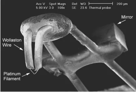
data acquisition. The scanner is linked to a feedback mechanism to maintain a constant force and the probe temperature is controlled by a wheatstone bridge so that an isoforce topographic image and an isothermal appar-ent thermal conductivity image can be simultaneously recorded. The thermoresistive probe derived from Din-widdies et al.’s work [6] comprises a Wollaston lever arm at the end of which the Platinum thermoresistive element is fixed. The heating tip is a simple filament of Platinum/10% Rhodium curved in V-shaped (Figure 1)

[7].

After positioning the probe on the sample’s surface, a scan is performed at constant force and temperature. Mallarino et al. [8] show an example of apparent thermal conductivity image obtained after scanning a unidirec-tional glass fibre reinforced composite in transverse di-rection. Localized thermomechanical measurements in-tended to determine melting point and glass transition temperature in polymer or composite can then be per-formed at high temperature rate (10 - 20 K/s) on selected points of the scan. The high rate limits the HAZ dimen-sions for a given material diffusivity. The probe dis-placement is then followed versus temperature [8].

In this example, sensor position successively increases showing sample thermal expansion at glassy state, and decreases drastically around 100˚C showing sample sof-tening after glass transition temperature [8].

2.2. Heat Exchange between the Probe and the Sample

The quality of measurements is closely related to the nature of the contact zone between the platinum probe and the surface of the sample. It is therefore important to well-understand the thermal exchanges associated to this localized measurement in order to quantify heat transfers and consequently the HAZ. In a previous work, Shi et al.

Figure 1. Micrograph of the thermal probe developed by Dinwiddie et al. [6,7]

conducted a detailed study of the thermal mechanisms that take place in the contact area between the thermo-couple tip and a hot substrate [9]. Type and shape of the probe and sample, atmospheric environment and distance between the probe and the sample are the parameters to be considered. Existing literature brings back a lot of works [9-11] describing the presence, below 100˚C, of a water meniscus which appears at the periphery of the probe tip and in the cavities created between probe and sample surfaces in the contact zone. In her PhD work [12], Gomes states that the heat exchange through the water meniscus is predominant. The intensity of this ex-change is directly linked to the thermal conductivity of the sample.

Consequently, three ways can be considered for de-scribing heat transfers (Figure 2)

o Transfer by conduction (probe/sample and probe/

water/sample);

o Transfer by natural convection (air/sample);

Transfer by radiation (probe/sample).

The involvement of radiation in the heat balance is not significant compared to the natural convection with air [13]. A modelling of the thermal behaviour of the probe of the Scanning Thermal Microscope (SThM) has re-cently been proposed by Grossel et al. [14]. The thermal exchange along the probe was modelled as a convection gradient of which the heat transfer coefficient value h is maximal at the periphery of the probe/sample contact area (with h = 1200 W/m2_{/K at the end of the probe in}

contact with the sample and h = 60 W/m2_{/K at the other}

end [15]). A similar study has proposed h values lying between 950 and 1300 W/m2_{/K [16].}

2.3. Contact Area between the Probe and the Sample

The HAZ will closely be related to the size of the contact area between the probe and the sample. Using analytical models, several authors have been able to quantify the dimensions of this contact area. So, Gomes et al. [16]

Sensor 

Sample 

Water meniscus 

Convective exchange 

Water Conduction exchange 

Sensor/Sample Conduction exchange 

Radiation exchange 

The thermal probe is replaced by a simplified thermal condition applied to the sample surface: the temperature increase of 15 ˚C/s (thermal loading of the probe) is sup-posed to be applied on a small surface of the sample equivalent to the probe contact area. The radius of this area is fixed at 80 nm according to the results of Gomes

et al. [16] and the presence of the water meniscus is not taken into account in the first step. The initial tempera-ture of the sample is fixed by a prescribed temperatempera-ture equal to 30˚C. The heat flux q on the top of sample sur-face due to convection is governed by boundary convec-tion:

estimate a circular contact surface with a 80 nm radius and a concentric circular water meniscus surface with an outside radius of 306 nm. As for Lefèvre et al. [17-19], they have suggested contact radii values ranging from 200 nm to 1 µm depending on temperature and probe geometry.

3. Numerical Approach and Results

Numerical models developed here are based on a 500 nm radius and 1 mm height cylindrical sample (geometrical models have been described by an axisymmetric repre-sentation – 2D½). Although the approach presented here is dedicated to study polymer materials, metal and ce-ramic materials have been chosen for several reasons. First, below 30˚C and 150˚C, their thermal properties can be considered as independent of the temperature. Then, close to 110 - 130˚C, mechanical properties of polymer materials decrease strongly and the thermal probewould push in the sample. So, the contact surface between the probe and the sample increases and must be considered in simulations. These phenomena are not considered here and will be taken into account in a future work where coupled thermomecanical simulations will be used.



q h  



with q: heat flux across the surface,

h: reference film convection coefficient,

θ: temperature at this point on the surface,



θ0_{: reference sink temperature value.}

Radiation heat exchange is not taken into account (not significant compared with convection exchange). Figure 3 summarized boundary conditions and thermal loading

applied to the model.

The sample is considered as thermally affected if the temperature of the area concerned reaches values higher or equal to 50˚C. The HAZ has been defined as the dis-tance between the centre of the probe and the thermal isovalue of 50˚C in the material. This value of 50˚C was chosen as reference because polymer properties are not affected below glass transition temperature (generally Tg

> 60˚C).

Table 1 summarizes the type and properties of the

materials that have been studied. Note that theses materi-als are supposed to be homogenous and isotropic.

The finite element models were realized with Abaqus code and the numerical models are meshed with 400 000 linear axisymetric heat transfer quadrilateral elements. A gradient element size (small: 16 nm × 16 nm / large: 6 × 6 µm) was realized to have a fine discretization under the

probe zone. 3.1. Influence of the Materials Physical Properties on the Zize of the HAZ A transient heat transfer analysis is applied, and heat

conduction is assumed to be governed by the Fourier law (Equation (1))

Solving the heat transfer equations related to a thermal problem only requires three materials properties: density, thermal conductivity and specific heat. In this part of the study, the aim is to identify the properties that are really influent on the size of the HAZ.

f k

x

   

 (1)

with k: matrix of conductivity, k = k(θ),

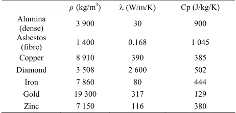
Figure 4 shows the thermal gradient at the end of

thermal loading in two samples, a heat insulation (asbes-tos) and a thermal conductor (copper). The quantity of material thermally impacted is more important in the radial direction than in the longitudinal one. For example, in the case of asbestos, a gap nearing 10% can be calcu-lated between the radial and the longitudinal lengths whereas for copper, the difference is only about 3%. Considering this first result, the shape of the HAZ can therefore be described by a hemispherical shape for thermal conductor materials. While for thermal insulator materials, a hemi-elliptical shape is more appropriate. Later, in this paper, only the radial length on the top sur-face of the sample is studied.

f: heat flux.

Table 1. Physical properties of materials used for modelling [20].

ρ(kg/m3_{)  (W/m/K) Cp (J/kg/K)}

Alumina

(dense) 3 900 30 900

Asbestos

(fibre) 1 400 0.168 1 045

Copper 8 910 390 385

Diamond 3 508 2 600 502

Iron 7 860 80 444

Gold 19 300 317 129

Zinc 7 150 116 380

1 mm

80 nm

Temperature load at

to 150°C 15°C.s-1 _between

30°C

Convection h=1200W.m-2_.K-1

Convection h = 1200 W/m2_/K

Temperature load at 15 ˚C /s between 30˚C to 150˚C

Initial temperature

T0 = 30°C 500µm

Figure 3. Boundary conditions and thermal load for numerical model.

 _80 nm 

(a)

(b)

Figure 4. Thermal gradient evolution in the sample at the end of thermal loading, i.e. Tprobe = 150˚C for asbestos (a) and copper

Figure 5 presents, at the end of thermal loading (Tprobe

= 150˚C), temperature variations along the horizontal upper surface (that is in contact with the probe) of the different model samples. Except for diamond, samples dimensions (1 mm × 1 mm) are enough to define a satis-fying representative elementary volume (REV) for mod-elling µ-TA process. The HAZ is increases with the dif-fusivity (Figure 6). Moreover, a linear evolution is found

between its size and the value of diffusivity.

The evolution of the HAZ versus thermal conductivity can also be well described by a linear interpolation as shown on Figure 7.

The other two parameters, specific heat and density, have been studied as a function of the HAZ (Figure 8 and Figure 9 respectively). It is difficult to use these results

to quantify the HAZ since they could not be interpolated by a mathematical function.

3.2. Influence of the Contact Zone

Calculations were carried out by considering different sizes of contact zone for different materials with different

30 50 70 90 110 130 150

0.00E+00 5.00E‐04 1.00E‐03 1.50E‐03 2.00E‐03

Te m p e ra tu re    (° C)

Length (mm)

Alumina Asbestos

Copper Diamond

Iron Gold

Zinc

Probe tip

Figure 5. Temperature evolution along the horizontal sur-face of the sample at the end of thermal loading; i.e. Tprobe =

150˚C (zoom in the contact zone with the thermal probe).

R² = 0.9467

0 0.1 0.2 0.3 0.4 0.5 0.6 0.7

0.0E+00 2.0E‐05 4.0E‐05 6.0E‐05 8.0E‐05 1.0E‐04 1.2E‐04 1.4E‐04

He a t   af fe ct ed   zo n e   (µ m )

Diffusivity (m2_.s‐1₎

Figure 6. Evolution of heat affected zone versus diffusivity.

R² = 0,9981

0 0.1 0.2 0.3 0.4 0.5 0.6 0.7

0 50 100 150 200 250 300 350 400

He a t   af fe ct e d   zo n e   (µm )

Thermal conductivity (W.m‐1_.K‐1₎

R2 _{= 0.9981}

Thermal conductivity (W/m/K)

Figure 7. Evolution of heat ffected zone versus thermal a conductivity.

R² = 0,5416

0 0.1 0.2 0.3 0.4 0.5 0.6 0.7

0 100 200 300 400 500 600 700 800 900 1000 1100

Hea t   af fe ct e d   zo n e   (µ m)

Specific heat (J.kg‐1_.K‐1₎

R2 _{= 0.5416}

Specific heat (J/kg/K)

Figure 8. Evolution of heat affected zone versus specific heat.

R² = 0,5295

0 0.1 0.2 0.3 0.4 0.5 0.6 0.7

0 5000 10000 15000 20000

Hea t   af fe ct e d   zo n e   (µ m)

Density (kg.m‐3₎

R2 = 0.5295

Density (kg/m3₎

Figure 9. Evolution of heat ne versus density.

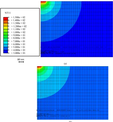
eat conductivities (copper, zinc, alumina and asbestos).

summarized on Figure 11. For thermal

in-su

affected zo

h

Figure 10 presents the numerical model used for these

calculations.

Results are

Diffusivity (m2_/s)

Contact zone

Temperature load at

Convection h= 1200 W.m-2_.K-1

15°C.s between 30°C to 150°C

-1

Initial temperature

T0 = 30°C

Figure 10. Numerical model used for study of the influence of the contact zone.

y = 3E‐09x2_{+ 3E‐06x + 0.0001}

R² = 0.9995 y = 0.0002e0.0083x

R² = 0.9975

y = 4E‐06x + 4E‐05 R² = 0.9997 0.E+00

2.E‐03 4.E‐03 6.E‐03 8.E‐03 1.E‐02 1.E‐02 1.E‐02

0 200 400 600 800 1000 1200

Si

ze

of

the

h

ea

t

af

fe

ct

e

d

zo

n

e

(m

m

)

Radius of the thermal tip (nm)

Alumina Copper zinc Asbestos

Figure 11. Evolution of heat affected zone versus contact

dius leads to a linear increase of the size of the HAZ in

of Water Meniscus

evelopment of the

ater me-ni

the corresponding nu

radius between the probe and the sample.

ra

the studied temperature range. For heat conductor mate-rials (zinc), the change in HAZ size with temperature is exponential.

3.3. Influence

The shape of the probe influences the d

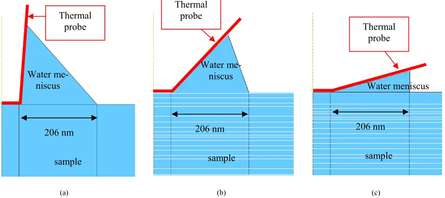
water meniscus. Three angles are arbitrary fixed for the probe in the study: 15˚, 45˚ and 85˚ (Figure 12). The

length of the contact zone between the meniscus and the sample is constant and equal to 206 nm whatever the angle of the probe is [16]. The thermal condition used in previous simulation was applied on a newprobe contact area (the sample surface and the water meniscus surface in contact with the thermal probe – Figure 12).

The contact zone between the sample and w

scus is perfect and no dissipation is allowed. Using the same type of elements as previously, a new meshing was realized. A particular attention was paid to the meshing of the contact zone with thermal probe, and that of water meniscus. Their discretization has been made with small sized elements in order to optimize the results.Boundary

conditions and thermal loading applied to numerical models are summarized in Figure 13.

Figure 14 presents the results of

Convection h = 1200 W/m2_/K

Temperature load at _{merical calculations. From a certain value of thermal}

conductivity, the role of water meniscus becomes less important. Taking into account the water meniscus in calculations leads to an increase of the HAZ of 27% for alumina and only less than 5% for zinc. On the other hand, when the material has a low thermal conductivity (as for asbestos), the presence of water meniscus leads to an increase of the HAZ from 3 to 5 times depending on the angle of the tip.

4. Discussion

15 ˚C/s between 30˚C to 50˚C

1

The finite element method enables to determine the

in-itial contact area of the probe is a cr

eir shapes are het-er

p

cus that drastically increases the size of the HAZ for heat fluence of intrinsic or external parameters on the size of the zone really thermally affected during a micro thermal analysis (HAZ). The development of simple model rep-resentative of matrices with very different thermal prop-erties is enough to define influent parameters such as thermal conductivity. From above results (Figure 7), it

should be possible to estimate the size of the HAZ from thermal conductivity measurements after calibrating the

μTA on several reference samples of well known thermal conductivities. Concerning specific heat which is diffi-cult to quantify experimentally, no influence has been found on final result.

As expected, the in

itical parameter on final HAZ size as observed on Fig-ure 11. The interest of FEM analysis here is to quantify the influence of contact size on HAZ depending on ther-mal conductivity. For heat conducting materials, the ex-ponential dependence between contact size and HAZ size requires the smallest possible contact areas. The techno-logical development of micro thermal analysis then needs a miniaturization of this contact zone. As an example, Depasse et al. [21] refer to some 30 nm radius for this zone. This study however deals with an 80 nm radius according to Gomes et al.’s work [10,12,16] that are more successfully completed in regard to the analysis and the understanding of classical micro thermal analysis measurements with standard probes.

Since the probes are handmade, th

menis-(a) (b) (c)

Figure 12. Probes and water meniscus profiles for the different numerical models: probe angle of 85˚ (a), 45˚ (b) and 15˚ (c).

80 nm

Temperature load at 15°C.s-1 _between 30°C to 150°C

Convection h= 1200 W.m-2_.K-1

Initial temperature

T0 = 30°C

Water meniscus (= 15°, 45° or 85°)

206 nm 

Contact Tied at the interface water meniscus / sample

Figure 13. Numerical model used for study of the influence of the water meniscus.

sulator materials (such as asbestos). The thermal

con-aracterization is usually difficult to

terials, this work led to the quantification of the heat af-in

ductivity of water is in fact more important than that of the heat insulator material, what interferes with localized measurements. It is therefore fundamental to take this phenomenon into account for this materials family.

5. Conclusions

Making localized ch

obtain. The physical parameters and the behaviours of materials are in fact modified compared to the macro-scopic scale. So, it is an important challenge to be able to quantify at this small scale the thermal and mechanical stresses occurring on materials. Using numerical simula-tion and considering the heat insulator or conductor

ma-fected zone during a localized micro thermal analysis. From the study of several parameters and conditions, the thermal conductivity has been found to be the driving physical parameter in thermal exchanges. It has therefore been possible to rapidly estimate the heat affected zone. Models showed that the water meniscus that appears at the interface between the probe and the sample has only little influence on the size of the heat affected zone for heat conductor materials. On the contrary, for heat insu-lator materials, this meniscus can lead to an increase of the size of the heat affected zone from 3 to 5 times. The contact angle has a limited influence on conductor mate-rials and a higher influence on insulators. Finally, owing

206 nm

sample

Water meniscus Thermal

probe

206 nm

sample Water

me-niscus Thermal

probe

206 nm

sample Water

me-niscus Thermal

probe

Temperature load at

Convection h = 1200 W/m2/K 15 ˚C/s between 30˚C to

0.E+00 2.E‐04 4.E‐04 6.E‐04 8.E‐04 1.E‐03 1.E‐03 1.E‐03 2.E‐03

0 100 200 300 400

He

a

t

af

fe

ct

e

d

zo

n

e

(mm)

Thermal conductivity (W. m‐1_.K‐1₎

500 probe angle: 15° probe angle: 45° probe angle: 85° without water meniscus

Figure 14. Evolution of heat affected zone for different shapes of probe an ater meniscus.

diversified techno-gical developments, the probes will probably m

pl

[1] E. Gmelin, R. , “Sub-Microm

Thermal Phys HM Techniques,”

d w

to their varying shapes coming from

lo odify

the water meniscus and the size of the heat affected zone. This work is just a first study on the topic of heat af-fected zone. In a near future, it will be necessary to com-ete it by defining new models that would describe mul-tiphased materials and to quantify the corresponding heat affected zones surrounding different phases.

REFERENCES

Fischer and R. Stitzinger ics—An overview on ST

eter

Thermochimica Acta, Vol. 310, No. 1-2, 1998, pp. 1-17.

doi:10.1016/S0040-6031(97)00379-1

[2] H. M. Pollock and A. Hammiche, “Micro-Therma Analysis: Techniques and Applications,” Journal ofl Physics D: Applied Physics, Vol. 34, 2001, pp. R23-R53.

doi:10.1088/0022-3727/34/9/201

[3] A. Altes, R. Tilgner and W. Walter, “Numerical Evalua-tion of Miniaturized Resistive Probe for Quantitative Thermal Near-Field Microscopy of Thermal Conductiv-ity,” Microelectronics Reliability, Vol. 46, No. 9-11, 2006, pp. 1525-1529. doi:10.1016/j.microrel.2006.07.030

[4] I. W. Rangelow, T. Gotszalk, N. Abedinov, P. Grabieca and K. Edingerb, “Thermal Nano-Probe,” Microelec-tronic Engineering, Vol. 57-58, 2001, pp. 737-748.

doi:10.1016/S0167-9317(01)00466-X

[5] D.-W. Lee and I.-K. Oh, “Micro/Nano-Heater Integ Cantilevers for Micro/Nano-Lithography Applications,” rated

Microelectronic Engineering, Vol. 84, No. 5-8, 2007, pp. 1041-1044. doi:10.1016/j.mee.2007.01.104

[6] R. Dinwiddie, R. Pylkki and P. West, “Thermal Conduc-tivity Contrast Imaging with a Scanning Thermal Micro-scope,” Thermal Conductivity, Vol. 22, 1994, pp. 668-677. [7] P. G. Royall, V. L. Kett and C. S. Andrews and D. Q. M. Craig, “Identification of Crystalline and Amorphous Re-gions in Low Molecular Weight Materials Using Mi-crothermal Analysis,” The Journal of Physical Chemistry B, Vol. 105, 2001, pp. 7021-7026.

doi:10.1021/jp010441k

[8] S. Mallarino, J. F. Chailan and J.

Investigation in Glass Fibre Composites by Micro-Thermal L. Vernet, “Interphase Analysis,” Composites Part A: Applied Science and Manufacturing, Vol. 36, No. 9, 2005, pp. 1300- 1306.

doi:10.1016/j.compositesa.2005.01.017

[9] L. Shi and A. Majumdar, “Thermal Transport Mec nisms at Nanoscale Point Contacts,”

ha-Journal of Heat Transfer, Vol. 124, 2002, pp. 329-337.

doi:10.1115/1.1447939

[10] S. Gomés, N. Trannoy and P. Grosse Microscopy: Study of th

l, “D.C. Thermal e Thermal Exchange between a

le Résistive,”

on

between a Hot Tip and a Substrate,”

C Modeling of the SThM Probe and a Sample,” Measurement Science and Tech-nology, Vol. 10, No. 9, 1999, pp. 805-811.

[11] S. Lefèvre, “Modélisation et Élaboration des Métrologies de Microscopie Thermique à Sonde Loca

Thermal conductivity (W/m/K)

Ph.D. Dissertation, Poitiers University, Poitiers, 2004. [12] S. Gomes, “Contribution Théorique et Expérimentale à la

Microscopie Thermique à Sonde Locale: Calibrati d’Une Pointe Thermorésistive, Analyse des Divers Cou-plages Thermiques,” Ph.D. Dissertation, Reims Univer-sity, Reims, 1999.

[13] S. Lefèvre, S. Volz and P. O. Chapuis, “Nanoscale Heat Transfer at Contact

International Journal of Heat and Mass Transfer, Vol. 49, No. 1-2, 2006, pp. 251-258.

[14] P. Grossel, O. Raphaël, F. Depasse, T. Duvaut and N. Trannoy, “Multifrequential A

Probe Behaviour,” International Journal of Thermal Sci-ences, Vol. 46, No. 10, 2007, pp. 980-988.

doi:10.1016/j.ijthermalsci.2006.12.004

[15] V. T. Morgan, “The Overall Convective

from Smooth Circular Cylinders,” Advances in Heat Heat Transfer Transfer, Vol. 11, 1975, pp. 199-264.

doi:10.1016/S0065-2717(08)70075-3

[16] S. Gomes, N. Trannoy, P. Grossel, F. D and D. Charraut, “D.C. Scanning Th

epasse, C. Bainier ermal Microscopy: Characterization and Interpretation of the Measurement,”

International Journal of Thermal Sciences, Vol. 40, 2001, pp. 949-958. doi:10.1016/S1290-0729(01)01281-9

[17] S. Lefèvre, S. Volz, J.-B. Saulnier, C. Fuentes and N. Trannoy, “Thermal Conductivity Calibration for Hot

f the Scanning Thermal Microscope in the

, No. 3,

nger-Verlag London, 2008.

. Wire Based DC Scanning Thermal Microscope,” Review of Scientific Instruments, Vol. 74, No. 4, 2003, pp. 2418-2423.

[18] S. Lefèvre, J.-B. Saulnier, C. Fuentes and S. Volz, “Probe Calibration o

AC Mode,” Vol. 35, No. 3-6, 2004, pp. 283-288. [19] S. Lefèvre and S. Volz, “3ω-Scanning Thermal

Micro-scope,” Review of Scientific Instruments, Vol. 76 2005, pp. 033701-033701-6.

[20] F. Cardarelli, “Materials Handbook—A Concise Desktop Reference,” 2nd Edition, Spri