American Open Journal of Statistics,2011, 1, 93-104
doi:10.4236/ojs.2011.12011 Published Online July 2011 (http://www.SciRP.org/journal/ojs)
Distributions of Ratios: From Random Variables to
Random Matrices
*
Thu Pham-Gia#, Noyan Turkkan
Department of Mathematics and Statistics, Universite de Moncton, Canada E-mail:#[email protected]
Received March 25, 2011; revised April 17, 2011; accepted April 25, 2011
Abstract
The ratio R of two random quantities is frequently encountered in probability and statistics. But while for
unidimensional statistical variables the distribution of R can be computed relatively easily, for symmetric
positive definite random matrices, this ratio can take various forms and its distribution, and even its
defini-tion, can offer many challenges. However, for the distribution of its determinant, Meijer G-function often
provides an effective analytic and computational tool, applicable at any division level, because of its repro-ductive property.
Keywords:Matrix Variate,Beta Distribution,Generalized-F Distribution, Ratios, Meijer G-Function, Wishart Distribution, Ratio
1. Introduction
In statistical analysis several important concepts and methods rely on two types of ratios of two independent, or dependent, random quantities. In univariate statistics, for example, the F-test, well-utilized in Regression and Analysis of variance, relies on the ratio of two indepen- dent chi-square variables, which are special cases of the gamma distribution. In multivariate analysis, similar pro- blems use the ratio of two random matrices, and also the ratio of their determinants, so that some inference using a statistic based on the latter ratio, can be carried out. La- tent roots of these ratios, considered either individually, or collectively, are also used for this purpose.
But, although most problems related to the above ra- tios are usually well understood in univariate statistics, with the expressions of their densities often available in closed forms, there are still considerable gaps in multi- variate statistics. Here, few of the concerned distributions are known, less computed, tabulated, or available on a computer software. Results abound in terms of approxi- mations or asymptotic estimations, but, as pointed out by Pillai ([1] and [2]), more than thirty years ago, asymp- totic methods do not effectively contribute to the practi- cal use of the related methods. Computation for hyper- geometric functions of matrix arguments, or for zonal polynomials, are only in a state of development [3], and,
at the present time , we still know little about their nu- merical values, to be able to effectively compute the power of some tests.
The use of special functions, especially Meijer G-fun- ctions and Fox H-functions [4] has helped a great deal in the study of the densities of the determinants of products and ratios of random variables, a domain not fully ex- plored yet, computationally. A large number of common densities can be expressed as G-functions and since products and ratios of G-functions distributions are again G-functions distributions, this process can be repeatedly applied. Several computer applicable forms of these functions have been presented by Springer [5]. But it is the recent availability of computer routines to deal with them, in some commercial softwares like Maple or Mathematica, that made their use quite convenient and effective [6]. We should also mention here the increasing role that the G-function is taking in the above two soft- wares, in the numerical computation of integrals [7].
special mathematical functions used in the previous sec- tion can all be expressed as G-functions, making the lat- ter the only tool really required.
In Section 4, extensions of the results are made in sev- eral directions, to several Wishart matrices and to the matrix variate Gamma distribution. Several ratios have their determinant distribution established here, for exam- ple the ratio of a matrix variate beta distribution to a Wishart matrix, generalizing the ratio of a beta to a chi square. Two numerical examples are given and in Sec-tion 5 an example and an applicaSec-tion are presented. Fi-nally, although ratios are treated here, products, which are usu- ally simpler to deal with, are also sometines studied.
2. Ratio of Two Univariate Random
Variables
We recall here some results related to the ratios of two independent r.v.’s so that the reader can have a compara-tive view with those related to random matrices in the next section.
First, for ~
, 2X X
X N
2
Y, independent of
~ Y,
Y N , RX Y has density established
nu-merically by Springer ([5], p. 148), using Mellin trans-form. Pham-Gia, Turkkan and Marchand ([8]) estab-lished a closed form expression for the more general case of the bivariate normal
,
~
, ; 2, 2;
X Y X Y
X Y N ,
using Kummer hypergeometric function . Sprin- ger ([5], p.156) obtained another expression but only for the case
1 1F .
0
X Y
.
The gamma distribution, X ~Ga
,
, with density
; ,
1exp
0g x x x ,x has as spe-
cial case Ga n
2, 2
called the the Chi-square with n degrees of freedom 2n
, with density :
1
/ 2
2
; exp 2 2 2 ,
n
n
g x n x x n x0.
With independent Chi-square variables 21 1~ n X and 2
2 2~ n
X , we can form the two ratios
1 1 1 2 and
W X X X W2 X1 X2 which have, re-
spectively, the standard beta distribution on [0,1] (or beta of the first kind I
1, 2
a
bet , with density defined on
0,1
by:
2 1
1 1
1 2
1 ,
f x x x B , 1, 20.
and standard betaprime distribution ( beta of the second kind II
1, 2
beta
) defined on
0, by
11
1 21, 2 1
f y y B y .
The Fisher-Snedecor variable F 1 2,
is just a multiple of the univariate beta prime W2.
For independent , we can form
the same ratios
~ , , 1
i i i
X Ga i , 2
1 1 1 2
T X X X and T2X1 X2.
the Generalized-F distribution,
2
T has T2 ~GF
, ,
,with density :
1
; , ,
, 1
t f t
B t
,
where 1, 2, 2 1 and we have
1,2 2 1 2 2
2, 2, 1
F T .
Naturally, when 12,
I1, 2
a
1~
T bet and
II
2 1,
T beta 2 .
Starting now from the standard beta distribution de-fined on (0,1), Pham-Gia and Turkkan [9] give the ex-pression of the density of R, and also of W X
XY
,using Gauss hypergeometric function . For the general beta defined on a finite interval (a,b), Pham-Gia and Turkkan [10] gives the density of R, using Appell’s function
2 1F .
.D
F , a generalization of . In [11],
several cases are considered for the ratio X/Y, with
2 1F .
,
~
Y Ga . In particular, the Hermite and Tricomi
functions, H
. and
. , are used. TheGeneral-ized-F variable being the ratio of two independent gamma variables, its ratio to an independent Gamma is also given there, using
. . Finally, the ratio of two independent Generalized-F variables is given in [11], using Appell function FD
. again. All these operationswill be generalized to random matrices in the following section.
3. Distribution of the Ratio of Two Matrix
Variates
3.1. Three Types of Distributions
Under their full generality, rectangular (p × q) random matrices can be considered, but to avoid several difficul-ties in matrix operations and definitions, we consider only symmetric positive definite matrices. Also, here, we will be concerned only with the non-singular matrix, with its null or central distribution and the exact, non-asymp- totic expression of the latter.
For a random (p × q) symmetric matrix, , there are three associated distributions. We essentially distin-guish between:
1
p
1) the distribution of its elements (i.e. its p p
1 2
independent elements eij in the case of a symmetric matrix), called here its elements distribution (with matrix input), for convenience. This is a mathematical expres-sion relating the components of the matrix, but usually, it is too complex to be expressed as an equation (or several equations) on the elements eijthemselves and hence, most often, it is expressed as an equation on its determi-nant.
(de-T. PHAM-GIA ET AL. 95
noted here by X instead of det
X ) (with positive real input), called determinant distribution, and3) the distribution of its latent roots (with p-vector in-put), called latent roots distribution.
These three distributions evidently become a single one for a positive univariate variable, then called its den-sity. The literature is mostly concerned with the first dis-tribution [12] than with the other two. The focal point of this article is in the determinant distribution.
3.2. General Approach
When dealing with a random matrix, the distribution of the elements within that random matrix constitutes the first step in its study, together with the computation of its moments, characteristic function and other properties.
Let X and Y be two symmetric, positive definite inde-pendent (p × q) random matrices with densities (or ele-ments distributions) fX
X and . As in uni-variate statistics, we first define two types of ratios, type I of the form
fY Y
X X Y, and type II, of the form: X Y . However, for matrices, there are several ratios of type II that can be formed: 1
1
Z XY , 1 and
2
Z Y X
1 2 1 2
Z3 Y X Y , where
T
Y1 2 is the symmetric
square root of Y, i.e. Y Y1 2
1
U 5
2 =Y
T 1, beside the two formed with the Cholesky decomposition of Y,
4
and1
T
Z U X Z V
1T
X
Y
V , where U is upper triangular, with , and V, lower tri-angular, with .
UU
=Y T VV
1) For elements distribution, we only consider Z3,
which is positive and symmetric, but there are applica-tions of 4 and 5 in the statistical literature. We can
determine the matrix variate distribution of Z3 from
those of X and Y. In general, for two matrix variates A and B, with joint density
Z Z
, ,
fA B A B
the density of1 2
B 1 2
G A A is obtained by a change of variables:
1 2,
A G , with dA associated
with all elements of A. When A and B are independent,
we have .
, p d
G A A
h G
AfG A
A
G A
f , , fB GA fA A
Gupta and Kabe [13], for example, compute the den-sity of G from the joint density g
A B, , using theap-proach adopted by Phillips [14].
1 1 2 2 11 22
11 22 22
11
, d
p
g K
F G F G
G F F
F F ,
where in the block division of A, 11 12 , we
21 22
A A
A
A A
have: A11
pp
,A22
q q
while
F21,F22
22
A
is the joint characteristic function of A21 et .
For
,
exp
+
2 1 2 12
n p q p
tr
g K
A B
A B A B ,
they obtained
2 1 2q p n q
g K
G G I G , i.e.
II ,
2 2
q n Beta
G .
Similarly, for Type I ratio, we can also have 5 types of ra- tios, and we will consider
1/ 2
1 2Ts
U X Y X X Y ,
the symmetric form of the ratio X X Y
1 for ele-ments distribution.2) In general, the density of the determinant of a ran-dom matrix A , can be obtained from its elements dis-tribution f
. of the previous section, in some simplecases, by using following relation for differentials:
1 d
A A A A
d tr ([15], p. 150). In practice, fre-quently, we have to manipulate A directly, often us-ing an orthogonal transformation, to arrive at a product of independent diagonal and off-diagonal elements.
The determinants of the above different ratios
i,i1, ,5
Z , have univariate distributions that are iden-tical, however, and they are of much interest since they will determine the null distribution useful in some statis-tical inference procedures.
3) Latent roots distributions for ratios, and the distri-butions of some associated statistics, remain very com-plicated, and in this article, we just mention some of their basic properties. For the density of the latent roots
l1, , lp
, we have, using the elements density f
. :
2 2
1
1
π
, , d ,
2
p p
T
p i j
i j
p O p
p
h l l l l f HLH H
p
l l
where O p
is the orthogonal group, H is anor-thogonal
pp
matrix,
dH
is the Haar invariantmeasure on O p
, and Ldiag
l1, , lp
([16], p. 105).3.3. Two Kinds of Beta, of Wilks’s Statistic, and of Latent Roots Distributions
We examine here the elements, determinant and latent roots distributions of a random matrix called the beta matrix variate, the homologous of the standard univariate beta.
First, the Wishart distribution, the matrix generalization of the chi-square distribution, played a critical part in the development of multivariate statistics. V ~Wp
n,C
, iscalled a Wishart Matrix with parameters n and C if its density is:
1 2
n p2 1 2np/ 2 n/ 2
p
f etr n
V C V V C 2 (1)
> 0,n p
1
p21
pf etr
W C W W C (2)
with W 0,C
pp
0 and
p1 2
Hence, If S W~ p
n,
, then S G~ ap
n 2, 2
.THEOREM 1: Let A W~ p
mA,
et B W~ p
mB,
, with A and B independent
pp
mA
positive definite symmetric matrices, and and mB integers, with
. Then, for the three above-mentioned dis-tributions, we have:
,
mA mB p
3.3.1. Elements Distribution
1) The ratio U
A B
1 2A A B
1 2 has the ma-trix beta distribution I
2, 2p
beta mA mB
, with densitygiven by (3).
2) Similarly, the ratio V B1 2AB1 2 has a
II 2, 2
p
beta mA mB
distribution if =Ip and B1 2is symmetric. Its density is given by (4).
3.3.2. Determinant Distribution
1) For U~betap
mA,mB
, its determinant U has Wilks’s distribution of the first type, denoted by
I
~ 2 mAmB , , 2p m
U B (to follow the notation
in Kshirsagar [17], expressed as a product of independent I
beta , and its density, is given by (5).
2) For V ~betapII
mA,mB
, its determinant V has Wilks’s distribution of the second type, denoted by
m m , , 2p mII A B
~ 2
V B , expressed as a product
of p independent univariate beta primes , and its density is given by (6).
II
beta
3.3.3. Latent Roots Distribution
1) The latent roots of U: The null-density of the latent roots
f1, , fp
of
1 2 1 2
U A B A A B or
is:
1B A A
1 2 2 1 2 1 2 1 1 2 2 1 , , π 2 , 1 p i pn p n p
p
i i i j
i i j
C p n C p n f l
p C p n n
f f f f
defined in the sector f1 f2 fp0, with
1 2 , 2 2 pni i p n C p ni
,
where
1
1
π 1 4
2
p
p
j
j
v p p v
,(If n1 p
but , we can make the changes
to obtain the right ex-pression).
2
n p
p n n, ,1 2
n p n1, , 1n2p
2) The latent roots of V: For GB1 2AB1 2 or
1
AB
, the roots
l1, ,lp
have density:
1 2
1 2 1 2 1 2 1 π 2 , 1 p i p n n p p n
i i i j
i i j
C
p C p n n
l l l l
1 2 , ,
p n C p n
f l
We have also: li fi
1 fi
.PROOF: The proofs of part 1) and part 3) are found ks in multivari analysis. For part 2, see [6
e results.
utions: The positive definite U has a beta distribution of the
in most textboo ate
]. QED.
The following explicative notes provide more details on the abov
3.4. Explicative Notes 1) On Elements Distrib symmetric random matrix first kind, ~ I
,p
beta a b
U if its density is of the form:
1 1 2
b p
-1 1 2
( , 0 < < , , a p p I f a b
) = p
p
U
U U I
β (3)
It has a beta of the second kind distribution, den by
U
oted
II
~beta a b,
V p if its density is of the form:
1 2
| |
p n
V
( ) ,0 < ( , ) | |a b
p p
f
a b
V V
β I V (4)
where a b,
p1
2, are positive real numbers, and
a b,p
β is the beta function in Rp,
i.e.
, p
p
a b
p , with
a b
a b
p
β
4 11
1
i
π
2
p p p
p i a a
.The transformations from I
, to pbeta a b
U~
II
~betap a b,
V
sim
also called the
and vice-ve le ones, Also, beta prime is rsa are simp
se, where the ilarly to the univariate ca
gamma-gamma distribution, frequently encountered in Bayesian Statistics [11], ~ II
,p
beta a b
V
can also be obtained as the continuous mixture of two Wishart densities, in the sense of V ~Wp
n,Ω
, with
0,
p
W n 0
Ω~ Ω . Also, for U and V above,
I
~ ,
p beta b a
I U and 1~
bet
V
eral case where
II
a b a, .
2) For the gen Ip, V is not nec-II
p
beta
essarily , as p out b ubin [18].
Se
ointed y Olkin and R dependen
veral other reasons, such as its cy on and on (A + akes V difficult to use, and Perlman [19] suggested using
B), m
1 2 1 1 2 II
* = + + ~betap mA 2,mB 2
V A B B A A B
which does not h
considering its elements distribution. 2) On Determinant Distributions: a) For
ave these w We will use this definition as the matrix ratio type II of A and B when
T. PHAM-GIA ET AL. 97
I
~betap m mA, B
U its determinant U has Wilks’s
distribution of the first type, denoted by
A B
, , 2p mB
(to follow the notation in[17]), expressed as a product of p univar
has been treated fully in [6]. This result is obtained via a transformation and by considering the elements on the diagonal.
I
~ 2 m m
U
with
1
1
1 1
2 2 2 2
p
j A
j j
n q q
.
iate betas of the first kind, and this expression
PROPOSITION 1
In the general case can have non-integral values and we can also have the case .
, ,
n p q
q p
PROOF: See (6).
REMARK: The cdf of Y is expressible in closed form, using the hypergeometric function 2 1F of matrix
argu-ment. ([12], p. 166) and the moments are : For integers n p, and q, with
n q p,
a) The density of the ratio U ~I
n,p q,
, is: (see (5)).where
,h p p
p p
a h b h
a b
E Y for
1
1 2
p
1 2
i
n i
K
n q i
.b) For
1 2
1 2
a p h b p
3) On Latent Roots distributions:
The distribution of the latent roots
f1, , ,f2 fp
of
I
~betap a b X
II
~betap m mA, B
V , the latent roots of AB1, 1
B A, and B1 2AB1 2 are the same, and so are the three determinants, and V can be expressed as a ct of p t univariate beta primes, which, in turn, can be expressed as Meijer’s G-functions, i.e.
produ independen
II
~Λ 2 mAmB , , 2p mB
V , or the Wilks’s
distribu-tion of the second type . Hence, for the above ratio V
1
,0 j j
T
V p V , with
II 1 1
~ ,
2 2
A B
j
m j m j
T beta
,
where
, was made almost at the same time by five distinguished statisticians, as we all know. It is sometimes referred to as the generalized beta, but the marginal distributions of some roots might not be uni-variate beta. Although they are difficult to handle, par-tially due to their domain of definition as a sector in , their associations with the Selberg integral, as presented in [20], has permitted to derive several important results. A similar expression applies for the latent roots of
p R
II
~betap a b,
Y .
4. Extensions and Generalizations
II
~ ,
X beta if it has as univariate density
1
1 1 1 1
1
, 1
( ,1) 1
( 1,1) x
From the basic results above, extensions can be made
into several directions and various applications can be found. We will consider here elements and determinant distributions only. Let us recall that for univariate distri-butions there are several relations between the beta and the Dirichlet, and these relations can also be established for the matrix variate distribution.
f x
B x
x
H
(6)
PROPOSITION 2: Wilks’s statistic of the second kind, II
, ,
, has as density (see (7)).n p q
1 1
1, 1, , 1
2 2 2
, 0
1 1
1, 1, , 1
2 2 2
0, 0
p p p p
n p
n n
K u
u
n q p
n q n q
h u
u
G
(5)
1 1
, , ...,
2 2 2 2 2
3 1
1, , ...,
2 2 2 2 2
p p p p
q q q p
f x A x
n q n q n q p
4.1. Extensions
4.1.1. To Several Matrices
There is a wealth of relationships between the matrix variate Dirichlet distributions and its components [12], but because of space limitation, only a few can be pre-sented here. The proof of the following results can be
und in [18] and [19], where the question of independ-idual ratios and the sum of all matri-ces is discussed.
tics, if fo
ence between indiv
1) In Matrix-variate statis
S S0, , ,1 Sk
are (k + 1) independent (p × p) random Wishart matrices,
~ ,
i Wp ni Σ
S , then, the matrix variates
k1 i iU ,
de-fined “cumulatively” by:
1 2 0 0 1 = + + + +k k k k
k
U S S S S
S S
are mutually independent,
1 2 1 2
1 0 1 1 0 1
1 2 1 2
0 0
= + + , ,
= + + + + , ,
j j j j
U S S S S S
U S S S S S
1 2 0 0 + , = + S U S
with , having a
matrix variate beta distrib.
2) Similarly, as suggeste ng,
, 1, , j j k U
I ,
p n nj o n Perlman [19], defi
j1
beta .
d by ni
1 2
1
1 2o o -1 o
= + + + + + +
j j j j
V S S S S S S Sj
then j and are mutually
inde inants, we have:
THEOREM 2
II
2 1
~ ,
j beta n nj o n V
pendent. Concerning their determ : Let
S S0, , ,1 Sk
s and
be (k + 1) indep (p × p) random Wishart matrice Uj and Vj
j defined as above. Then the two products
1 j i i
Ω U and 1 j j i i
Ω V 1 j k, as well as any ratio ,
j k jk
U U and V Vj k,jk, have the densities of their determinants expressed in closed forms in terms of Meijer G-functions.
PROOF : We have
1 I
~ 2 ,
j j
0 0
, 2
j nk
U ,
1 j k
k k k p n
II , , 2j1
0 0
~ 2 j
j nk p nk
, and the result isk k
V
immediate fro ion 2 of The
stributions given in the Appendix.
Ex ven here to save space bu
are a QED.
Also, considering the sum
m Sect orem 1 and the expres-sion of the G-function for products and ratios of inde-pendent G-function di
act expressions are not gi t
vailable upon request.
0
k j j
T S , if we take: 1 2 1 2
0 0
W T S T , 1 2 1 2
j j
W T S T and
1 2 1 2
0 0
j j
T W W W 1 j k ector
, then 1) the matrix v
W, ,Wk
ution, i.e 1
pe I distrib
has the matrix
variate Dirichlet of ty .
n nj,
I 1, , k ~Dir
W W 0 , with density:
0 1 n p
1
j
n p 2
2 1
1 1
, , k k j k j , j 0,
j j
f c
I
W W W W W
1 0 k j j
I W , where
0 , , i iC p n c
C p n
, with kk
0 j
j
n
nand
1 1 2 2 1 1 , 2 2 pn p
p p n j
j
C p n
and .
I ~ 2,j betap n n n 2
W .
2) the matrix v s trix variate
Dirich
i
ector k) ha the ma distribu , i.e.
i (T1, , T
tion let of type II
II
1, , k ~Dir n nj, 0
T T , with density:
1 2 1 1 2 1 1, , , 0
j n p k j j k n k k j j j f c j
I TT T T
T
and Ti ~beta
2
ni
2
. THEOREM 3II ,
p ni n
: Under the same hypothesis as the densities of the determinants of
rem 2 , i j
RW W i j and of R* T Ti j , can b tained sed form in terms of G-funct .
e ob
in clo ions
PROOF: We have
nin p n0, , 0
andI j W
0, , 0
II
j nin p n
T , 1 j k and the conclusion
is immediate from Section 2 of Theorem 1. QED.
4.1.2. To the Matrix Variate Gamma Distribution In the preceding sections we started with the Wishart distribution. However, it is a more g neral to consider the Gamma matrix variate distribution,
e
~Ga ,
W C .
, we know that Here
1
~ p i i
X
WC , with independent
1
~ ,1
i
i
X Ga . Hence, the density of W
2
is :
p 0 1, 3, ,f w K 0 pw 1 , 0
2 2 p w G C (8) with 1 p 1 1 2 i i
K
.
Although for two independent Matrix Gammas, 1
and W2, their symmetric ratio of the second type,
W
1 2 1 2
2 1 2
diffi-T. PHAM-GIA ET AL. 99
ecommendatio
ma n be implem
w stribution o
Matrix variate
culty as with the Wishart, the same r ns de by Perlman [19] ca ented to obtain the ell-defined elements di f the Generalized F
1 2
~GFp ,
W
butio
. The matrix variate -distri
,p
GF a b
,
II p
beta
n, a scaled form of the
just lik ratio of the t
, is encountered in m ariate counterpart. B
eterminants
ultivariate regression, ut we have, for the o d
e its univ w
1
1 1
p
i p i
1 2 p
i i
X T Y
W W W i, with independent
i II
1 2
1 1
~ ,
2 2
i
i i
T beta
(9)
Hence, the distribution of W , the determinant of
1 2
~GFp ,
W has density:
2 2 2
1 2 1 1
1 , , 1
2 2
3 1
1 , , ,
2 2
p p p p
p
x
p
G
,
f z A
(10)
with
1
1 2 2
, which is
1
1 1
2
p
j
j j
A
of the same form as (4).
The determinants of the product and ratio of the two
p
GF
given i
variates, can now be computed, using th
n the Appendix, extending the univariate case
es [1
4.2. Further Matrix Ratios
There are various types of ratios encountered in the st tistical literature, extending the univariate results of Pham-Gia and Turkkan [21] on divisions by the univari-ate gamma variable. We consider the following four trix variates, which include all cases considered p
is a special case of ):
, with integer
Beta type II or e method
tablished for the generalized-F 1].
ma- revi-ously (
Let n,
2
θ Beta type I (beta
G
1
θ
θ 4
θ
1~Wishart Wp ni,
I ,
p a b ), θ3
Fp(a,b) (BetaII
a b, or GFp
a b, ), a b,
p1 2
,Gamma
,C
, (Gap
,C
, 0,C0).The elements distributions of various products
4
θ
1 2 1 2
j i j
θ θ θ , and ratios 1 2 1 2
j i j
θ θ θ and
1 2
1 2i j i i j
1i j, 4, can be carried out, bu
θ θ θ θ θ , for independent
t will usually lead to ,
i j θ θ ,
quite complex results. Some results when both θi and
j
θ are θ2-matrices are obtained by Bekker, Roux and
Pham-Gia [22].
However, for their determinants, we have:
2
1 1
1
p
n i i
θ ,
I I
2
1
~ 2 , ,
2 2
j
a b eta a b
p b, 2 ~ b j 1 ,
θ
II 2
a b
II
3
1 1 ~ 2 b , ,p ~
beta a j ,b j θ ,
2 2
4 1
1
~ ,
2
p
i
1
C
θ .
The exp
i ga
ressions of the densities of θi ,1 i 4, in
terms of G-functions are given in previous sectio s, ex-pt for
n ce 1 the density of which is given by (12) below.
I θ
and II here are generalized Wilks’s variables, with a and b positive constants, instead of being integers.
THEOREM 4: For any of the above matrix variates j
θ
1 ,
i j
a) The density of the determinant of any product = θ θi j , and ratio
2 ,
i j
= θ θi j , 0i j, 4 s of Meijer G
, in the unc
above list, can be ex in term -f
tions.
b) Furthermore, subject to the independence of all the factors involved, any product and ratio of different
pressed
-and of different i j 1,
,1 4
i i
θ , and i j ,2 ,
0i j, 4, can also hav e pressed in
terms of G-functions.
e their d nsities ex
PROOF: The proof is again based on t tive
property of the Meijer G-functions when product and ratio ope ons are performed, with the complex
expres-ns for se operations presented in [6], and reduced in the Appendix. Computation details can be pro-vi
he reproduc
rati
sio the
ded by the authors upon request. QED.
REMARK: Mathai [23] considered several type f integ equations ass ilks’ work and pro-vide solutions to these equations in a general theoretical context. The method presented here can be used to give a
G-s o
ral ociated with W
5. Example and Application
function or H-function form to these solutions, that can then be used for exact numerical computations.
We provide here an example using Theorem 4, with two graphs and also an engineering application.
5.1. Example
Let betaIIni, ,p ni ,i 1, 2
. Th
~
i
θ
2 2
p e densities of Y =
1 2
θ θ and R = 1 2
θ
θ can be obtained in closed form as
1, 1 1 , , 1 1 1
2 2 2 2
q q q p
2 2 2 2
1 2
1 1
, , ,
2 2 2 2
1 1
3 3
2 2 2 2 2 2
q q q p
n q n q n q p
(11)
1 2
p p p , 1 2
p p p p
f y A y
G
1 1 1, 1 1 , , 1 1
2 2 2 2
2 2 2 2 2 2
2 2
1, , ,
n q n q n q p
1
1
1 1
2 2 2 2
i P
i j
i i i
A
j j
n q q
for y0 with AA A and
,i1, 2.
Similarly, the ratio R has density:
1 1 1 1 2 2 2 2 2 2 2
1 1 1 1 1 1 1 2 2 2 2
1 1
1 1
, , , , , ,
2 2 2 2 2 2 2 2 2 2
1 1
3 p p
n 3
1, , , 1 , , ,
2 2 2 2 2 2 2 2 2 2
p p
q q q p n q n q n q p
f r A r
n q n q q p q q q p
G
(12)
fo
PROOF r r0.
: Using (7) above, we can derive (11) and (12) by applying the approach presented in the Appendix.
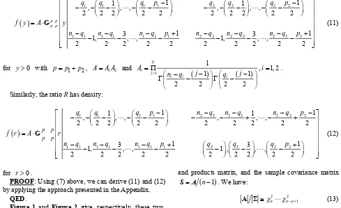
[image:8.595.53.542.84.383.2]QED.
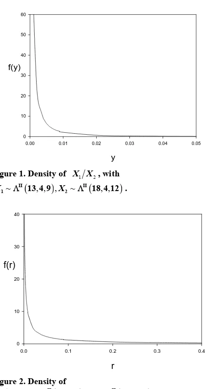
Figure 1 and Figure 2 give, respectively, these two
densities, for and
18, usin
5.2. Application to Multivariate Process Control
n-do le of
1 2 4, 1 9, 2 12, 1 13
p p q q n g the MAPLE software.
2
n
1) Ratios of Variances: The generalized variance is treated in [24]. We consider X ~Np
μ,Σ
and a ram samp
X1, , XN
X. We define
X X
X
, the sample sum o sand products matrix, and the sample covariance matrix
n 1
S A . We have:
2 2
1
n n p
A (13) where the 2
j
variables, with j degrees of freedom, 1
n p j n are independent. This is also the distribution of p
n S
1
.
Now let S and S2 be tw
ices of sizes
o independent sample
co-variance m and respectively.
From (1), ve atr
we ha 1
n n2
~ 1, 1 .
i p n ni
S W
a) The sam le generalized riance p vai i
1
N T
Α X f square
1
pii i
n
i i
Y S has density:
1
0
00
2
2
p
j i
i n j
h y
G 2 , 3 , , 1 , 02 2 2
2p
n n
y
(14)
1 1 p i
p i
n p
y
) Now, the two types of ratios V
p
0, yi 0,i1, 2
2
= 1 2 1 2 2 S1 2
S S and U =
S1S2
1 2S S1
1S2
1 2,
0 0
~Np μ , can be determined.We have I
1 2
~Beta n 1 2, n
U 1 2 and
I
1 2 2
~ n n 2, ,p n
U
not necessarily
1 . V has a density which is
II
1 1 2, 2 1 2
Beta n n , but we
have: II
1 2 2
~ n n 2, ,p n
V 1 .
Application: In an industrial environment we wish to monitor the variations of a normal process
X , using the variations of the ratio of two variance matrices taken from that en-ainst the fluctuations of its control envi-ro
random sample co vironment, ag
nment Y~Np
μ0,0
, represented by a similar ratio. ceed in several sta) Let
For clarity, we will pro eps: and S2
1 2
X
θ S S , with S1 being two
random samples of sizes n1 and n2 from
0, 0
pN μ
2) and, similarly, θY S3 S4 , with S3
T. PHAM-GIA ET AL. 101
60
y
0.00 0.01 0.02 0.03 0.04 0.05
f(y)
[image:9.595.65.279.69.466.2]0 10 20 30 40 50
Figure 1. Density of X X1 2, with
~ , , , ~ II , ,
1 13 4 9 X2 18 4 12 . II
X
r
0.0 0.1 0.2 0.3 0.4
f(r)
[image:9.595.73.399.80.711.2]0 10 20 30 40
Figure 2. Density of
1 2, ~ , , , ~ , ,
II II
1 13 4 9 2 18 4 12
X X X X .
from Np
μ Σ,
. Hence,
II
3 4 4
3 4
II
1 2 1 2 2
II 3 4
1
II 1 2
1
2, , 1
2, , 1
1 1, 1 1
2 2 2 2
1 1, 1 1
2 2 2 2
Y
X p
i p
i
n n p n
n n p n
n i n i
beta
n i n i
beta
S S
θ
θ S S
b) For the denominator, its density is given by (7):
1 1 2
2 2
2
1
p pr
1 1
1
2 2
2 1
, , ,
2 2 2
2 3 4
, , ,
2 2 2
p
j
p p g x
n j n j
n n p
n
n p
n n
G
and similarly for the numerator.
c) Applying the ratio rule in the Appendix for these two independent G-function distributions, we have the
y of
densit . QED.
6. Conclusions
As shown in this article, for several types of random ma-trices, the moments of which can be expressed in terms of gamma functions, Meijer G-function provides a pow-erful tool to derive, and numerically compute, the
densi-tie ese
matrices. Multivariate hypothesis testing based on de-terminants can now be accurately carried out since the expressions of null distributions are, now, not based on asymptotic considerations.
7. References
[1] K. C. S. Pillai, “Distributions of Characteristic Roots in Multivariate Analysis, Part I: Null Distributions,”
Com-ory and Methods, Vol. 4,
r
un tions in Statistics—Theory and Methods, Vol. . 21, 1977, pp. 1-62.
Edelman, “The Effective Evaluation of etric Function of a Matrix Argument,” Mathematics of Computation, Vol. 75, 2006, pp. 833-846.
s of the determinants of products and ratios of th
munications in Statistics—The No. 2, 1976, pp. 157-184.
[2] K. C. S. Pillai, “Distributions of Characteristic Roots in Multiva iate Analysis, Part II: Non-Null Distributions,”
m ica
Com 5, No
[3] P. Koev and A.
the Hypergeom
doi:10.1090/S0025-5718-06-01824-2
[4] A. M. Mathai and R. K. Saxena, “Generalized
Hyper-geometric Functions with Applications in Statistics and Physical Sciences,” Lecture Notes in Mathematics, Vol. 348, Springer-Verlag, New York, 1973.
[5] M. Springer, “The Algebra of Random Variables,” Wiley, New York, 1984.
[6] T. Pham-Gia, “Exact Distribution of the Generalized
Wilks’s Distribution and Applications,” Journal of Muo- tivariate Analysis, 2008, 1999, pp. 1698-1716.
“The Evaluation of Integrals of Bessel G-Function Identities,”Journal of
Compu-[7] V. Adamchik,
Functions via
tational and Applied Mathematics, Vol. 64, No. 3, 1995, pp. 283-290.doi:10.1016/0377-0427(95)00153-0
[8] T. Pham-Gia, T. N. Turkkan and E. Marchand,
“Distribu-tion of the Ratio of Normal Variables,” Communica-
tions in Statistics—Theory and Methods, Vol. 35, 2006, pp. 1569-1591.
[9] T. Pham-Gia and N. Turkkan, “Distributions of the Ratios of Independent Beta Variables and Applications,” Com- munications in Statistics—Theory and Methods, Vol. 29, No. 12, 2000, pp. 2693-2715.
doi:10.1080/03610920008832632
of General Beta Distributions,” Statistical Papers, Vol. 43, No. 4, 2002, pp. 537-550.
doi:10.1007/s00362-002-0122-y
[11] T. Pham-Gia and N. Turkkan, “Operations on the
Gener-5-209.
alized F-Variables, and Applications,” Statistics, Vol. 36, No. 3, 2002, pp. 19
doi:10.1080/02331880212855
[12] A. K. Gupta and D. K. Nagar, “Matrix Variate Distribu-tions,” Chapman and Hall/CRC, Boca Raton, 2000. [13] A. K. Gupta and D. G. Kabe, “The Distribution of
Sym-metric Matrix Quotients,” Journal of Multivariate Analy-sis, Vol. 87, No. 2, 2003, pp. 413-417.
doi:10.1016/S0047-259X(03)00046-0
[14] P. C. B. Phillips, “The Distribution of Matrix Quotients,” Journal of Multivariate Analysis, Vol. 16, No. 1, 1985, pp. 157-161.
doi:10.1016/0047-259X(85)90056-9
ate Statistical The-[15] A. M. Mathai, “Jacobians of Matrix Transformations and
Functions of Matrix Argument,” World Scientific, Sin-gapore, 1997.
[16] R. J. Muirhead, “Aspects of Multivari ory,” Wiley, New York, 1982.
doi:10.1002/9780470316559
[17] A. Kshirsagar, “Multivariate Analysis,” Marcel Dekker, New York, 1972.
[18] I. Olkin and H. Rubin, “Multivariate Beta Distributions and Independence Properties of the Wishart Distribu-tion,” Ann
1964, pp. 261-269.
als Mathematical Statistics, Vol. 35, No.1,
1177703748 doi:10.1214/aoms/
“The Multivaraite Selberg Beta
Distribu-0802185372
[19] M. D. Perlman, “A Note on the Matrix-Variate F Distri-bution,” Sankhya, Series A, Vol. 39, 1977, pp. 290-298.
[20] T. Pham-Gia,
tion and Applications,” Statistics, Vol. 43, No. 1, 2009, pp. 65-79. doi:10.1080/0233188
“Distributions of Ratios of
plications,” Statistics, Vol. 39, No. 4,
etoria,
s
[21] T. Pham-Gia and N. Turkkan,
Random Variables from the Power-Quadratic Exponen-tial family and Ap
2005, pp. 355-372.
[22] A. Bekker, J. J. J. Roux and T. Pham-Gia, “Operations on the Matrix Variate Beta Type I Variables and Applica-tions,” Unpublished Manuscript, University of Pr Pretoria, 2005.
[23] A. M. Mathai, “Extensions of Wilks’ Integral Equation and Distributions of Test Statistics,” Annals of the Insti-tute of Statistical Mathematics, Vol. 36, No. 2, 1984, pp. 271-288.
![N [(2 Chlorophenyl)sulfonyl] 3 nitrobenzamide](data:image/gif;base64,R0lGODlhAQABAIAAAP///wAAACH5BAEAAAAALAAAAAABAAEAAAICRAEAOw==)