Proceedings of the 49th Annual Meeting of the Association for Computational Linguistics:shortpapers, pages 625–630,
A Scalable Probabilistic Classifier for Language Modeling
Joel Lang
Institute for Language, Cognition and Computation School of Informatics, University of Edinburgh
10 Crichton Street, Edinburgh EH8 9AB, UK [email protected]
Abstract
We present a novel probabilistic classifier, which scales well to problems that involve a large number of classes and require training on large datasets. A prominent example of such a problem is language modeling. Our classifier is based on the assumption that each feature is associated with a predictive strength, which quantifies how well the feature can predict the class by itself. The predictions of individual features can then be combined according to their predictive strength, resulting in a model, whose parameters can be reliably and effi-ciently estimated. We show that a generative language model based on our classifier consis-tently matches modified Kneser-Ney smooth-ing and can outperform it if sufficiently rich features are incorporated.
1
Introduction
A Language Model (LM) is an important compo-nent within many natural language applications in-cluding speech recognition and machine translation. The task of a generative LM is to assign a probabil-ityp(w)to a sequence of wordsw =w1. . . wL. It is common to factorize this probability as
p(w) =
L
Y
i=1
p(wi|wi−N+1. . . wi−1) (1)
Thus, the central problem that arises from this formulation consists of estimating the probability
p(wi|wi−N+1. . . wi−1). This can be viewed as a
classification problem in which the target word Wi corresponds to the class that must be predicted, based on features extracted from the conditioning context, e.g. a word occurring in the context.
This paper describes a novel approach for mod-eling such conditional probabilities. We propose a classifier which is based on the assumption that each feature has a predictive strength, quantifying how well the feature can predict the class (target word) by itself. Then the predictions made by individual features can be combined into a mixture model, in which the prediction of each feature is weighted ac-cording to its predictive strength. This reflects the fact that certain features (e.g. certain context words) are much more predictive than others but the pre-dictive strength for a particular feature often doesn’t vary much across classes and can thus be assumed constant. The main advantage of our model is that it is straightforward to incorporate rich features with-out sacrificing scalability or reliability of parame-ter estimation. In addition, it is simple to imple-ment and no feature selection is required. Section 3 shows that a generative1 LM built with our classi-fier is competitive to modified Kneser-Ney smooth-ing and can outperform it if sufficiently rich features are incorporated.
The classification-based approach to language modeling was introduced by Rosenfeld (1996) who proposed an optimized variant of the maximum-entropy classifier (Berger et al., 1996) for the task. Unfortunately, data sparsity resulting from the large number of classes makes it difficult to obtain reli-able parameter estimates, even on large datasets and the high computational costs make it difficult train models on large datasets in the first place2.
Scal-1
While the classifier itself is discriminative, i.e. condition-ing on the contextual features, the resultcondition-ing LM is generative. See Roark et al. (2007) for work on discriminative LMs.
2
For example, using a vocabulary of20000words Rosen-feld (1994) trained his model on up to 40M words, however employing heavy feature pruning and indicating that “the com-putational load, was quite severe for a system this size”.
ability is however very important, since moving to larger datasets is often the simplest way to obtain a better model. Similarly, neural probabilistic LMs (Bengio et al., 2003) don’t scale very well to large datasets. Even the more scalable variant proposed by Mnih and Hinton (2008) is trained on a dataset consisting of only14M words, also using a vocabu-lary of around20000words. Van den Bosch (2005) proposes a decision-tree classifier which has been applied to training datasets with more than 100M words. However, his model is non-probabilistic and thus a standard comparison with probabilistic mod-els in terms of perplexity isn’t possible.
N-Gram models (Goodman, 2001) obtain esti-mates for p(wi|wi−N+1. . . wi−1) using counts of
N-Grams. Because directly using the maximum-likelihood estimate would result in poor predictions, smoothing techniques are applied. A modified inter-polated form of Kneser-Ney smoothing (Kneser and Ney, 1995) was shown to consistently outperform a variety of other smoothing techniques (Chen and Goodman, 1999) and currently constitutes a state-of-the-art3generative LM.
2
Model
We are concerned with estimating a probability dis-tribution p(Y|x) over a categorical class variable
Y with range Y, conditional on a feature vector
x = (x1, . . . , xM), containing the feature valuesxi ofM features. While generalizations are conceiv-able, we will restrict the featuresXk to be binary, i.e. xk ∈ {0,1}. For language modeling the class variableY corresponds to the target wordWiwhich is to be predicted and thus ranges over all possible words of some vocabulary. The binary input fea-turesx are extracted from the conditioning context
wi−N+1. . . wi−1. The specific features we use for
language modeling are given in Section 3.
We assume sparse features, such that typically only a small number of the binary features take value
1. These features are referred to as the active fea-tures and predictions are based on them. We troduce a bias feature which is active for every in-stance, in order to ensure that the set of active fea-tures is non-empty for each instance. Individually, each active featureXkis predictive of the class vari-able and predicts the class through a categorical
dis-3
The model of Wood et al. (2009) has somewhat higher per-formance, however, again due to high computational costs the model has only been trained on training sets of at most 14M words.
tribution4distribution, which we denote asp(Y|xk). Since instances typically have several active features the question is how to combine the individual pre-dictions of these features into an overall prediction. To this end we make the assumption that each fea-ture Xk has a certain predictive strength θk ∈ R, where larger values indicate that the feature is more likely to predict correctly. The individual predic-tions can then be combined into a mixture model, which weights individual predictions according to their predictive strength:
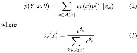
p(Y|x, θ) = X
k∈A(x)
vk(x)p(Y|xk) (2)
where
vk(x) =
eθk
X
k∈A(x)
eθk (3)
HereA(x) denotes the index-set of active features for instance(y, x). Note that since the set of active features varies across instances, so do the mixing proportionsvk(x)and thus this is not a conventional mixture model, but rather avariableone. We will therefore refer to our model as the variable mixture model (VMM). In particular, our model differs from linear or log-linear interpolation models (Klakow, 1998), which combine a typically small number of components that arecommon across instances.
In order to compare our model to the maximum-entropy classifier and other (generalized) linear models, it is beneficial to rewrite Equation 2 as
p(Y =y|x, β) = 1
Q(x)
M
X
k=1 |Y|
X
j=1
φj,k(y, x)βj,k (4)
= 1
Q(x)β
>φ(y, x) (5)
where φj,k(y, x) is a sufficient statistics indicating whether featureXkis active and classy=yj and
βj,k =eθk+logp(yj|xk) (6)
Q(x) = X
k∈A(x)
[image:2.612.312.540.218.307.2]eθk (7)
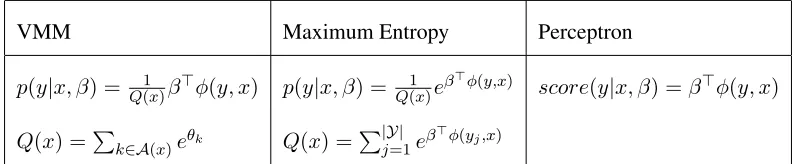
Table 1 shows the main differences between the VMM, the maximum-entropy classifier and the per-ceptron (Collins, 2002).
4
VMM Maximum Entropy Perceptron
p(y|x, β) = Q(1x)β>φ(y, x) p(y|x, β) = Q1(x)eβ>φ(y,x) score(y|x, β) =β>φ(y, x)
Q(x) =P
k∈A(x)eθk Q(x) = P|Y|
j=1eβ
>φ(y
[image:3.612.107.504.72.154.2]j,x)
Table 1: A comparison between the VMM, the maximum-entropy classifier and the perceptron. Like the perceptron and in contrast to the maximum-entropy classifier, the VMM directly uses a predictorβ>φ(y, x). For the VMM the sufficient statisticsφ(y, x)correspond to binary indicator variables and the parametersβare constrained according to Equation 6. This results in a partition functionQ(x)which can be efficiently computed, in contrast to the partition function of the maximum-entropy classifier, which requires a summation over all classes.
2.1 Parameter Estimation
The VMM has two types of parameters:
1. the categorical parameters αj,k = p(yj|xk) which determine the likelihood of class yj in presence of featureXk;
2. the parameters θk quantifying the predictive strength of each featureXk.
The two types of parameters are estimated from a training dataset, consisting of instances(y(h), x(h)). Parameter estimation proceeds in two separate stages, resulting in a simple and efficient procedure. In a first stage, the categorical parameters are com-puted independently for each feature, as the maxi-mum likelihood estimates, smoothed using absolute discounting (Chen and Rosenfeld, 2000):
αj,k =p(yj|xk) =
c0j,k
ck
wherec0j,kis the smoothed count of how many times
Y takes value yj when Xk is active, and ck is the count of how many times Xk is active. The smoothed count is computed as
c0j,k =
(
cj,k−D ifcj,k >0 D·N Zk
Zk ifcj,k = 0
where cj,k is the raw count for class yj and fea-ture Xk, N Zk is the number of classes for which the raw count is non-zero, andZk is the number of classes for which the raw count is zero. D is the discount constant chosen in [0,1]. The smoothing thus subtractsDfrom each non-zero count and re-distributes the so-obtained mass evenly amongst all zero counts. If all counts are non-zero no mass is redistributed.
Once the categorical parameters have been com-puted, we proceed by estimating the predictive strengthsθ = (θ1, . . . , θM). We can do so by con-ducting a search for the parameter vectorθ∗ which maximizes the log-likelihood of the training data:
θ∗= arg max
θ ll(θ)
= arg max
θ
X
h
logp(y(h)|x(h), θ)
While any standard optimization method could be applied, we use stochastic gradient ascent (SGA, Bottou (2004)) as this results in a particularly conve-nient and efficient procedure that requires only one iteration over the data (see Section 3). SGA is an online optimization method which iteratively com-putes the gradient∇for each instance and takes a step of sizeηin the direction of that gradient:
θ(t+1) ←θ(t)+η∇ (8)
The gradient∇ = (∂ll∂θ(h)
1 , . . . , ∂ll(h)
∂θM )computed for SGA contains the first-order derivatives of the data log-likelihood of a particular instance with respect to theθ-parameters which are given by
∂ ∂θk
logp(y|x, θ) = vk(x)
p(y|x, θ)[p(y|xk)−p(y|x, θ)]
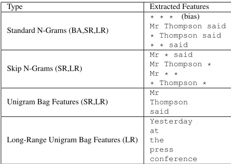
Type Extracted Features
Standard N-Grams (BA,SR,LR)
* * * (bias)
Mr Thompson said
* Thompson said * * said
Skip N-Grams (SR,LR)
Mr * said Mr Thompson * Mr * * * Thompson *
Unigram Bag Features (SR,LR)
Mr Thompson said
Long-Range Unigram Bag Features (LR)
Yesterday at
[image:4.612.71.303.71.236.2]the press conference
Table 2: Feature types and examples for a model of order N=4 and for the contextYesterday at the press conference Mr Thompson said. For each fea-ture type we write in parentheses the feafea-ture sets which include that type of feature. The wildcard symbol*is used as a placeholder for arbitrary regular words. The bias feature, which is active for each instance is written as* * *. In standard N-Gram models the bias feature corresponds to the unigram distribution.
update depends on how much overall and feature prediction differ and on the scaling factor vk(x)
p(y|x,θ).
In order to improve generalization, we estimate the categorical parameters based on the counts from all instances, except the one whose gradient is being computed for the online update (leave-one-out). In other words, we subtract the counts for a particular instance before computing the update (Equation 8) and add them back when the update has been ex-ecuted. In total, training only requires two passes over the data, as opposed to a single pass (plus smoothing) required by N-Gram models.
3
Experiments
All experiments were conducted using the SRI Lan-guage Modeling Toolkit (SRILM, Stolcke (2002)), i.e. we implemented5the VMM within SRILM and compared to default N-Gram models supplied with SRILM. The experiments were run on a 64-bit,2.2
GHz dual-core machine with 8GB RAM.
Data The experiments were carried out on data from the Reuters Corpus Version 1 (Lewis et al.,
5The code can be downloaded from http://code.
google.com/p/variable-mixture-model.
2004), which was split into sentences, tokenized and converted to lower case, not removing punctuation. All our models were built with the same 30367 -word vocabulary, which includes the sentence-end symbol and a special symbol for out-of-vocabulary words (UNK). The vocabulary was compiled by se-lecting all words which occur more than four times in the data of week 31, which was not otherwise used for training or testing. As development set we used the articles of week 50 (4.1M words) and as test set the articles of week 51 (3.8M words). For training we used datasets of four different sizes: D1 (week 1,3.1M words), D2 (weeks 1-3,10M words), D3 (weeks 1-10,37M words) and D4 (weeks 1-30,
113M words).
Features We use three different feature sets in our
experiments. The first feature set (basic, BA) con-sists of all features also used in standard N-Gram models, i.e. all subsequences up to a lengthN −1
immediately preceding the target word. The sec-ond feature set (short-range, SR) consists of all ba-sic features as well as all skip N-Grams (Ney et al., 1994) that can be formed with theN−1length con-text. Moreover, all words occurring in the context are included as bag features, i.e. as features which indicate the occurrence of a word but not the partic-ular position. The third feature set (long-range, LR) is an extension of SR which also includes longer-distance features. Specifically, this feature set ad-ditionally includes all unigram bag features up to a distanced = 9. The feature types and examples of extracted features are given in Table 2.
Model Comparison We compared the VMM to
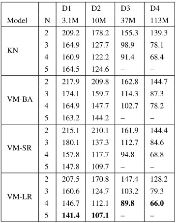
D1 D2 D3 D4
Model N 3.1M 10M 37M 113M
KN
2 209.2 178.2 155.3 139.3 3 164.9 127.7 98.9 78.1
4 160.9 122.2 91.4 68.4 5 164.5 124.6 – –
VM-BA
2 217.9 209.8 162.8 144.7
3 174.1 159.7 114.3 87.3 4 164.9 147.7 102.7 78.2
5 163.2 144.2 – –
VM-SR
2 215.1 210.1 161.9 144.4 3 180.1 137.3 112.7 84.6
4 157.8 117.7 94.8 68.8 5 147.8 109.7 – –
VM-LR
2 207.5 170.8 147.4 128.2
3 160.6 124.7 103.2 79.3 4 146.7 112.1 89.8 66.0
[image:5.612.95.274.70.297.2]5 141.4 107.1 – –
Table 3: The test set perplexities of the models for orders N=2..5 on training datasets D1-D4.
Model Parametrization We used the
develop-ment set to determine the values for the absolute dis-counting parameter D(defined in Section 2.1) and the number of iterations for stochastic gradient as-cent. This resulted in a valueD = 0.1. Stochas-tic gradient yields best results with a single pass through all instances. More iterations result in over-fitting, i.e. decrease training data log-likelihood but increase the log-likelihood on the development data. The step size was kept fixed atη = 1.0.
Results The results of our experiments are given
in Table 3, which shows that for sufficiently high orders VM-SR matches KN on each dataset. As ex-pected, the VMM’s strength partly stems from the fact that compared to KN it makes better use of the information contained in the conditioning con-text, as indicated by the fact that VM-SR matches KN whereas VM-BA doesn’t. At orders 4 and 5, VM-LR outperforms KN on all datasets, bringing improvements of around 10% for the two smaller training datasets D1 and D2. Comparing VM-BA and VM-SR at order 4we see that the7 additional features used by VM-SR for every instance signifi-cantly improve performance and the long-range tures further improve performance. Thus richer fea-ture sets consistently lead to higher model accuracy. Similarly, the performance of the VMM improves as one moves to higher orders, thereby increasing the amount of contextual information. For orders2and
3VM-SR is inferior to KN, because the SR feature set at order 2 contains no additional features over KN and at order 3 it only contains one additional feature per instance. At order 4 VM-SR matches KN and, while KN gets worse at order5, the VMM improves and outperforms KN by around14%.
The training time (including disk IO) of the or-der4VM-SR on the largest datasetD4is about30
minutes, whereas KN takes about6minutes to train.
4
Conclusions
The main contribution of this paper consists of a novel probabilistic classifier, the VMM, which is based on the idea of combining predictions made by individual features into a mixture model whose com-ponents vary from instance to instance and whose mixing proportions reflect the predictive strength of each component. The main advantage of the VMM is that it is straightforward to incorporate rich fea-tures without sacrificing scalability or reliability of parameter estimation. Moreover, the VMM is sim-ple to imsim-plement and works ‘out-of-the-box’ with-out feature selection, or any special tuning or tweak-ing.
Applied to language modeling, the VMM re-sults in a state-of-the-art generative language model whose relative performance compared to N-Gram models gets better as one incorporates richer fea-ture sets. It scales almost as well to large datasets as standard N-Gram models: training requires only two passes over the data as opposed to a single pass required by N-Gram models. Thus, the experiments provide empirical evidence that the VMM is based on a reasonable set of modeling assumptions, which translate into an accurate and scalable model.
Future work includes further evaluation of the VMM, e.g. as a language model within a speech recognition or machine translation system. More-over, optimizing memory usage, for example via feature pruning or randomized algorithms, would al-low incorporation of richer feature sets and would likely lead to further improvements, as indicated by the experiments in this paper. We also intend to eval-uate the performance of the VMM on other lexical prediction tasks and more generally, on other classi-fication tasks with similar characteristics.
Acknowledgments I would like to thank
References
Y. Bengio, R. Ducharme, P. Vincent, and C. Jauvin. 2003. A Neural Probabilistic Language Model. Journal of Machine Learning Research, 3:1137–1155.
A. Berger, V. Della Pietra, and S. Della Pietra. 1996. A Maximum Entropy Approach to Natural Language Processing. Computational Linguistics, 22(1):39–71. L. Bottou. 2004. Stochastic Learning. In Advanced
Lectures on Machine Learning, Lecture Notes in Ar-tificial Intelligence, pages 146–168. Springer Verlag, Berlin/Heidelberg.
S. Chen and J. Goodman. 1999. An Empirical Study of Smoothing Techniques for Language Modeling. Com-puter Speech and Language, 13:359–394.
S. Chen and R. Rosenfeld. 2000. A Survey of Smooth-ing Techniques for ME Models. IEEE Transactions on Speech and Audio Processing, 8(1):37–50.
M. Collins. 2002. Discriminative Training Methods for Hidden Markov Models: Theory and Experiments with Perceptron Algorithms. In Proceedings of the Conference on Empirical Methods in Natural Lan-guage Processing, pages 1–8, Philadelphia, PA, USA. J. Goodman. 2001. A Bit of Progress in Language Mod-eling (Extended Version). Technical report, Microsoft Research, Redmond, WA, USA.
D. Klakow. 1998. Log-Linear Interpolation of Language Models. InProceedings of the 5th International Con-ference on Spoken Language Processing, pages 1694– 1698, Sydney, Australia.
R. Kneser and H. Ney. 1995. Improved Backing-off for M-Gram Language Modeling. InProceedings of the International Conference on Acoustics, Speech and Signal Processing, pages 181–184, Detroit, MI, USA. D. Lewis, Y. Yang, T. Rose, and F. Li. 2004. RCV1: A New Benchmark Collection for Text Categorization Research. Journal of Machine Learning Research, 5:361–397.
A. Mnih and G. Hinton. 2008. A Scalable Hierarchical Distributed Language Model. InAdvances in Neural Information Processing Systems 21.
H. Ney, U. Essen, and R. Kneser. 1994. On Structur-ing Probabilistic Dependences in Stochastic Language Modeling. Computer, Speech and Language, 8:1–38. B. Roark, M. Saraclar, and M. Collins. 2007.
Discrimi-native n-gram Language Modeling. Computer, Speech and Language, 21:373–392.
R. Rosenfeld. 1994. Adaptive Statistical Language Mod-elling: A Maximum Entropy Approach. Ph.D. thesis, Carnegie Mellon University.
R. Rosenfeld. 1996. A Maximum Entropy Approach to Adaptive Statistical Language Modeling. Computer, Speech and Language, 10:187–228.
A. Stolcke. 2002. SRILM – An Extensible Language Modeling Toolkit. In Proceedings of the 7th Inter-national Conference on Spoken Language Processing, pages 901–904, Denver, CO, USA.
A. Van den Bosch. 2005. Scalable Classification-based Word Prediction and Confusible Correction. Traite-ment Automatique des Langues, 42(2):39–63.