Dynamic graph based search in unknown environments

Dynamic graph-based search in unknown environments

HAYNES, Paul, ALBOUL, Lyuba <http://orcid.org/0000-0001-9605-7228> and

PENDERS, Jacques <http://orcid.org/0000-0002-6049-508X>

Available from Sheffield Hallam University Research Archive (SHURA) at:

http://shura.shu.ac.uk/3755/

This document is the author deposited version. You are advised to consult the

publisher's version if you wish to cite from it.

Published version

HAYNES, Paul, ALBOUL, Lyuba and PENDERS, Jacques (2012). Dynamic

graph-based search in unknown environments. Journal of Discrete Algorithms, 12, 2-13.

Copyright and re-use policy

See http://shura.shu.ac.uk/information.html

Dynamic graph-based search in unknown environments

Paul S Haynes and Lyuba S Alboul and Jacques S Penders {p.haynes,l.alboul,j.penders}@shu.ac.uk 1

Abstract

A novel graph-based approach to search within unknown environments is presented. A virtual geometric structure is imposed upon the environment rep-resented in memory by a graph. Algorithms use this representation to coordinate a team of robots (or entities). Local discovery of environment features causes dynamic expansion of the graph resulting in global exploration of the unknown environment. The algorithm is shown to have O(n) time complexity, and a maximum bound on the length of the resulting walk Ω is given.

1. Introduction

The method presented in this paper stems from the research in multi-robot systems within the remits of the recently completed GUARDIANS project2_.

Autonomous mobile robotics, in particular collective and cooperative robotics, has gained a lot of attention recently.

Multi-robot systems pose new challenging problems such as cooperative per-ception and localization, cooperative task planning and execution, team navi-gation behaviors, robot interactions among themselves and with humans, coop-erative learning, and communication.

There have been some significant advances in tackling the aforementioned problems, often based, however, on empirical approaches. They are either driven by informal expert knowledge, or by resource-intensive trial-and-error processes [7].

There is a demanding need for formalization of methodologies and theoretical frameworks capable of providing solutions to general classes of problems specific for multi-robot systems.

In this paper such a framework is proposed for the problem of global self-localization of multi-robot teams, when noa priori information about the en-vironment is known.

The problem of self-localization is one of the central problems in robotics, and is particularly difficult in unknown indoor environments where such tools as GPS are unavailable.

2

It is directly related to the famous SLAM problem of a robot simultane-ously localizing and building a map of the environment. This problem has been studied extensively in the robotics literature, focusing mostly on a single robot. Conceptually, the SLAM problem for a single robot in 2D is considered to be solved, but in practice it may still encounter difficulties, even outdoors, in urban areas or forests. SLAM approaches are mainly probabilistic in their na-ture due to the uncertainty of acquired information. Data association methods used in SLAM require significant computation in real-life implementations, and contribute to increased complexity [8].

The problem of multi-robot localization and encountered difficulties has not yet been fully researched [9]. A multi-robot team, by definition, represents a sensor network. An important aspect of a multiple robotic system, as opposed to a single robot, is the richness of available information. In a cooperative multi-robot team, robots obtain information from their own sensors as well as other robots. This information can be of various types: perceptual (data from lasers, various distributed cameras) as well as non-perceptual (symbolic infor-mation, directions, and commands, obtained from other robots or a database). Therefore, richness of information should be taken into account.

In the last decade, several works appeared that tackle the problem of co-operative multi-robot localization. Whereas some approaches still consider this problem within the SLAM framework, by treating the problem of multi-robot localization as a Multi-SLAM problem [10], others, while still using probabilis-tic methods, attempt to take into consideration robots as landmarks themselves [11]. Another trend is based on robot distribution on site, which can work well if the group of robots is large and communication between them is robust [13]. A promising mathematical tool to characterize a multi-robot system is a graph. Indeed, the problem of coordination in multi-robot systems can be char-acterized naturally by a finite representation of the configuration space using Graph Theory. Nodes represent robots with resources limited by sensors, con-trol design, and computational power. Edges are virtual entities describing local interactions and can support information flow between nodes/robots. If other sensor devices are present in the environment they can be added to the sen-sor robot networks. Graph theory facilitates analysis of the interplay between the communications network and robot dynamics, and to choose strategies for information exchange which mitigate these effects.

Graph-theoretical approaches have been increasingly used for building and analyzing communication and sensor networks [14].

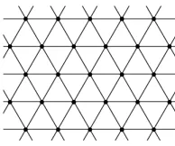
In this paper we describe a graph-theoretical framework for cooperative multi-robot localization. The (unknown) site is initially covered by an infinite virtual triangular grid (triangular tiling)T∞, depicted in Fig. 1.

The grid spans infinitely in all directions, and as robots explore the site local parts of the grid become actualized. The environment, therefore, represents a subgraphLofT∞. The robots are equipped with the Laser Range Finder (LRF) which is used as the main sensor for position detection with radio signal as a backup.

Figure 1: Virtual triangular grid

depending on the initial position of the robots. Our robot team consists of minimally three robots, and robots act as dynamic and static graph nodes; they switch between these two modes in a prescribed manner. Coordination of robots whilst correcting for odometry errors then becomes more manageable and a cooperative exploration algorithm has been developed.

The choice of three robots is due to several reasons. One is that this allows accurate calculation of robot positions and poses without assuming that robots are equipped with a proprioceptive motion detector as suggested in [11], as two robots act as static beacons whilst the third robot is moving. It also allows to develop a robust movement strategy that minimizes the number of robot steps. Indeed, our goal is not only to achieve robust self-localization of robots, but also explore the unknown environment in the most optimal manner, reducing the number of visits to previously visited nodes inL.

From a theoretical point of view, our method, to a certain extent, repre-sents a fusion and further development of strategies proposed in [16] and [15]. One crucial difference is that movements of the robots in our approach are not random, but are determined in a structured yet adaptive manner. The robots build the representation of the environment simultaneously whilst moving. For this reason, we consider the dual graphH∞toT∞; the nodes of this graph are possible positions of our 3-robot team considered as a whole.

Surprisingly, the result of the presented approach bears some similarity to that of [17] in which a Kohonen Self-Organizing Network (SOM) is used to obtain a topological graph representation of the environment. The SOM node positions change during network convergence, but the graph itself does not, i.e edges are not deleted. Our approach represents the environment better in the sense that unnecessary edges and nodes are removed and obstacles are repre-sented as cycles in the graph. A further advantage is a lower computational cost; neural network approaches can take a long time to converge. Moreover, the authors of [17] assume a perfect odometry, which is impossible in real-life applications.

2. Framework

The framework described here is intended to provide a discrete mathematical framework in which to achieve the following goals.

• Enable a team of 3 robots to autonomously explore an unknown environ-ment.

• To make no assumptions about the environment beyond the graph em-bedding.

• To cover the whole of the accessible environment (Completeness)

• To intelligently recognize and avert the visiting of “redundant” regions (viaIntelligent rules)

• To make deductions concerning the final walk length.

2.1. Localization and Movement Graphs

Our approach imposes a virtual geometric structure on the unknown envi-ronment, thus providing an environment coordinate system in which to develop algorithms. The structure is the infinite triangular grid graph T∞_{, chosen for} reasons discussed previously. The infinite hexagonal grid graphH∞_{dual toT}∞ is also necessary.

A localization graph is an induced subgraph L ⊂ T∞ used to represent possible robot locations. The unknown localization graph to be discovered is denotedL ⊂T∞, with the known graph denotedL⊂ L.

The 3-clique of robots progressively learn the unknown localization graphL as exploration proceeds untilL=L − L0_{, where L}0 _{is the indiscoverable graph,} at which point the algorithm terminates. At any one timeLis the learned lo-calization graph. The indiscoverableL0 _{pertains to enclosed inaccessible regions} of the environment. Likewise, an hexagonalmovement graph is an induced

sub-Figure 2: Robots ready for search. Surrounding unvisited localization vertices are identified. The dual movement graph is constructed accordingly.

M ⊂H∞, and the known movement graph denoted M⊂ M. The movement graphM is dual toL, and represents possible 3-clique movements governed by Rule (1) below.

Rule 1. Let C={Ri} ∈L be a 3-clique of vertices as in Figure (2), with cor-responding dual movement graph vertex m∈M. A single robot is permitted to move between two stationary robots. This move corresponds to an edge connect-ingmto some other vertexm0∈M (cf. Figure 3)

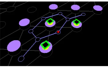
Figure 3: A single time step demonstrating dynamic extension.

The justification of Rule (1) stems from the problem of odometry error correction in real robots described earlier. This well known problem demands careful consideration of the approach to robot movement to minimize the accumulation of odometry error. Small errors in odometry result in large errors over long distances.

Algorithm 1. A1 Compute level-1face.

1: procedure _{ComputeOuterFace}(G)

2: Find left most vertexv∈G.

3: Letu= (0,1)

4: Findarg min

w

{∠(u,−→vw)|v−→w}

5: Lets=−→vw

6: f =v

7: whiles6=udo

8: f +w

9: Let u=−→wv, v=w

10: Find arg min

w

{_∠(u,−→vw)|v−→w}

11: end while

12: returnf

2.2. Movement

Vertices of the current localization graph L represents robots (here on re-ferred to as entities) within the environment. However, it is the movement graph

M, dual toL, which facilitates actual movement.

Our approach uses the principle of dynamic exploration (or search) through

M by moving from the current vertex to the next vertex on the outer face (also called a level-1 face [4]) of M. On moving to a new location L and M are updated and the process repeats.

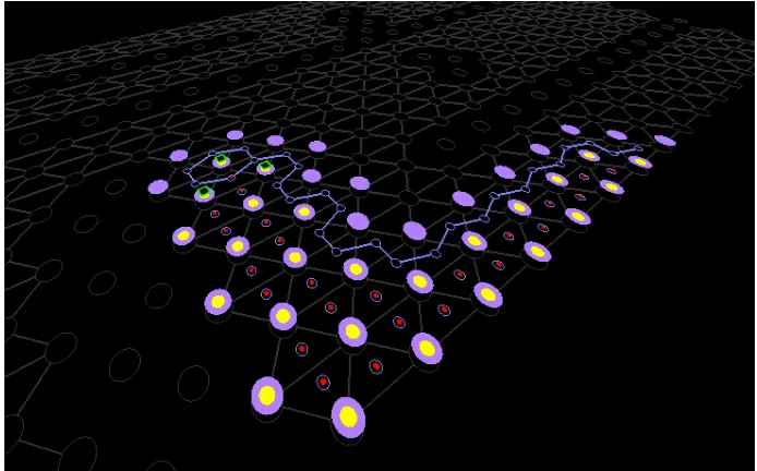
Figure 3 demonstrates updating after a move has occurred. The 3-clique of entities (green and black squares), are situated within the known localization graph L (denoted by large circles). The yellow circles on localization vertices represent visited vertices, whilst those without represent known (sensed) ver-tices. The known movement graphM (light blue) shows the moves available to the 3-clique (not necessarily from its current location). Red spots indicate those visited vertices ofM. The unknown localization graphLcan be seen here in grey.

As the 3-clique of entities move from vertexmto vertexm0 of the movement graph the source vertexm is removed from the graph if removal does not dis-connected the graph, i.e. removal is permitted if and only ifω(G\m) =ω(G), whereω(X) is the number of connected components of graph X. This simple principle of

• traversing the current outer face ofM;

• dynamically extendingL (and subsequently the dual graphM); and

• removing the source vertices where possible,

is a mechanism for automating the search of an unknown environment in an ordered manner. However, the geometric embeddings imposed on L and M

coupled with this simple principle of search means the path taken may not be optimal, and is discussed next.

2.3. Intelligent Rules

Besides the constraints imposed by the unknown environment (such as forc-ing the the movement graph to be 1-connected, for example), there are other situations in which the discussed simple principle of search may not be optimal. There may emerge, for example, a simple path of a level-1 face whose vertices are enclosed entirely by visited vertices. Clearly it would be inefficient for the entities to revisit such vertices since we may infer them as empty space. Indeed, since sensed vertices were actualized (i.e. there were no obstacles found), and they are surrounded by wholly visited nodes, then they may be inferred to be visited (since they are empty). A depth first search can quickly identify such regions and disconnect the located (possibly biconnected) region on back-tracking.

path proceeding from the current vertex is checked to see if it is enclosed by wholly visited vertices. If it is then the graph is disconnected at this vertex since traversing the path is unnecessary and would be inefficient. If not, then validation is complete and the entities must be allowed to traverse the path in order to visit the unexplored region.

3. Algorithms and Complexity

3.1. Nomenclature

The logical denotations True (>), False (⊥), and the logical AND operation over a set of discrete values (V_{) are used. The algorithms are presented from an}

object oriented perspective, thusa→_F()denotes that_F()is a member function of object (vertex)ato be called, for example. This should not be confused with the long arrow notationu −→ v, denoting vertices u and v of a graph to be connected by an edge.

TheComputeOuterFace()function computes the level-1 face (outer face) walk of M [4, 2], details of which are given in the next section. The resulting outer face walk is denoted Ω, with the current member denoted ω ∈ Ω. The next element of the walk is denotedω0 = ω+ 1. The list Ω is understood to be cyclic in thatωn+ 1 =ω1 andω1−1 =ωn, where ω1 and ωn are the first

and last elements of Ω respectively, and is implemented in C++ using the list container.

The current 3-clique of entities in the localization graphL are denotedRi,

wherei= 1,2,3. Position vectors associated with a vertex are denoteda→c, whereais a given vertex.

3.2. The level-1 face

Although simple, the level-1 face algorithm is given here for completeness. A vertexvis a level-kvertex if it is on the kth _{nested face, e.g. a level-1 vertex}

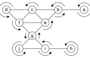
sits on the outer face. We call a cycle of level-kvertices a level-k face, [4]. Computing the level-1 face is equivalent to determining the outer face, for which there is a linear time algorithm. Figure 4 shows a connected triangular grid graphG⊂T∞. Finding the level-1 face begins with determining the left most vertexv∈G, vertexdin this case (if multiple vertices share this position then the most recently found is chosen).

Now consider a direction vector uparallel to the vertical axis. Vertex v is called the pivot and is the first vertex of the face. Determining the next vertex requires finding a vertexw−→v such that the anti-clockwise angle fromuto −→

vw is minimal, (f in this case).

Direction vectoruis then replaced byu=−→wv, and the pivot byw. Repeating the process sweeps out the face from vertex to vertex as shown untiluis equal to the initial edge.

The notation_∠(u,v) below denotes the anti-clockwise angle from vector u

Algorithm 2. 1: procedure _{DynamicSearch} . Searches an unknown environment.

2: ifgraph altered then. If the graph has been updated we must compute a new outer face walk

3: ω0 ← ∅

4: if Ω6=∅ then . If a previous walk exists

5: ω0 ←ω+ 1 . ω points to the next element in the walk

6: end if

7: Ω←(ω→ComputeOuterFace()) . Compute new walk

8: if ω06=∅ then

9: if there existsv∈Ωsuch that (v=ω)∧((v+ 1) =ω0)then .

Find exact position inΩif possible (should the local walk remain unchanged)

10: ω←v . Set current position

11: goto 16

12: end if

13: end if

14: Find ω0∈Ω such thatω0=ω . Since the local walk has changed, find any matching vertex

15: ω←ω0

16: end if

17: ifω→_ValidatePath(ω+ 1) then . Check necessity of path

18: graph altered← > . Redundant paths have been removed

19: goto 2

20: end if

21: ω←ω+ 1 . Move to next vertex in walk

22: Findi∈ {1,2,3} such thatRi6∈(ω→S) . Determine entity to move

23: Ri←(ω→S)\((ω−1)→S) . Move the entity

24: r←Ri .Remember which entity moved

25: r→visited← > . Set it as visited

26: ifhis not a cut-vertex then . Remove previously visited vertex?

27: Disconnect hfrom all neighbors.

28: end if

29: (ω→visited)← 3

^

i=1

(Ri→visited)

30: graph altered←(_{RealiseSurroundingArea}(r)>0). UpdateL and

M

31: for all3-cliquesCi∈L such thatr∈Ci and

^

c∈Ci

(c→visited)do .

Remove visited movement graph verticesv dual toCi

32: Let v∈M be the hexagonal vertex dual toCi.

33: if v6=ω then . Do not consider current clique

34: if v connects to any other verticesthen

35: Disconnect those vertices connecting to v which are not cut-vertices.

36: graph altered=>

37: end if

38: end if

39: end for

40: for allconnected neighborss∈N(r)such that ¬(s→visited)do

41: s→visited← ^

s0_∈N(s)

(s0→visited) . sbecomes visited if its

surrounding vertices are visited

42: end for

Figure 4: Simplified example of computing a level-1 (outer) face f1 = abcdf gjihigeb.

problem of an arbitrary set of points described in [3], but applied to embedded graphs in the plane.

3.3. Main Algorithms

The main algorithm to search an unknown environment is presented in the listing A2. The approach is partially inspired by the algorithms for hamiltonian walks in known environments, but adapted to unknown environments.

Details of hamiltonian walk construction in known environments for which no assumption is made as to thek-connectedness of the graph may be found in [2]. Optimal hamiltonian walks for known graphs that are at least 4-connected are well established (see Tutte [5, 6], for example)

Algorithm A2 is the starting point of the system, and has the following mechanisms:

(i) Computation of _{ComputeOuterFace(}·₎and the identification and tak-ing of the next move in the walk, or, if the graph local to the 3-clique remains unchanged, taking the next move in the current walk.

(ii) Checking whether the next move is actually necessary and removing (i.e. deleting) unnecessary simple paths viaValidatePath(·).

(iii) Disconnecting the previous vertexω−1 following a move toω if and only ifω−1 isnot a cut-vertex.

(iv) Dynamic expansion of the 3-clique frontier via_{RealiseSurroundingArea(}·₎, or similar.

(v) Maintaining the flagging of graph vertices as visited, either explicitly or implicitly.

For this last mechanism, note that explicit flagging occurs when a movement graph vertex is physically surrounded by the 3-clique, whereas implicit flagging occurs, for example, when a recently visited movement vertex has neighbors that are themselves surrounded by entirely visited vertices.

The complexity of algorithm A2 is given by the following proposition.

Algorithm 3. 1: procedure _{ValidatePath(}p₎ . Searches for and removes unnecessary paths.

2: avoid←this

3: ifp→_Recur() then

4: Disconnect pfromavoid.

5: return >

6: end if

7: return⊥

8: end procedure

9: procedure Recur()

10: rtn← >

11: visited← ^

s0_∈S

(s0 →visited)

12: this→visited← >

13: if¬visited then

14: return ⊥

15: end if

16: for allp∈N(this), p∈Ωsuch thatp6=avoidof this vertex do

17: if phas not yet been traversed by DFSthen

18: if (p→_Recur()) then

19: Disconnect pfrom all its neighbors.

20: else

21: rtn← ⊥

22: end if

23: end if

24: end for

25: returnrtn 26: end procedure

Proof. The first subroutine of algorithm A2 is_{ComputeOuterFace}() which computes the level-1 face of the current movement graphM. This is a simple

O(n) time algorithm as discussed in section 3.2.

Following computation of the level-1 face requires locating where in the new level face corresponds to the previous location in the previous level face so that we can take the next move. This takesO(|Ω|), wherenH ≤ |Ω| ≤2nH.

Path validation and removing of unnecessary paths via ValidatePath() takesO(nH) time (see proposition 2).

The remaining subroutines remove remaining implicitly visited regions local to the 3-clique. Finally, by Proposition 3 (see below), the RealiseSurroundin-gArea() subroutine has complexityO(1). Summing gives an overall complexity ofO(nH).

Algorithm A2 makes use of the _ValidatePath() function as discussed in the previous section, with complexity given by the proposition below.

Algorithm 4. 1: procedure _{RealiseSurroundingArea(}r₎.Dynamically extend the graph

2: P← ∅+{(ω→c, ω)}

3: r→known← >

4: for all 3-cliques Ci = {r, a, b} ∈ L where (¬(a → known))∧(b →

known)do

5: v→c← 1 3

X

c∈Ci

c→c . Makev∈M the dual vertex toCi∈L

6: v→visited← ^

c∈Ci

(c→visited)

7: v→S ←Ci

8: P ←P+{(v→c, v)}

9: end for

10: counter←0

11: for allelementss∈P do

12: for all elementst∈P such that allt proceedsdo

13: if k(s→c)−(t→c)k2<3/2 then . Is this a neighboring hexagonal vertex

14: if s 6−→t and s has not been previously disconnected from t

then

15: Connect stot. . Establish new connections (edges)

16: counter←counter+ 1

17: end if

18: end if

19: end for

20: end for

21: returncounter

22: end procedure

Proof. A level-1 face P ⊂ M has a maximum of nP < nH vertices. Since

algorithm A2 is effectively a depth first search ofP, its complexity isO(nP), or

more generally we may state that for any pathP algorithm A2 has complexity

O(nH).

The _{RealiseSurrouondingArea}() function depends on the application at hand. A robotics setting would require this function to physically scan the surrounding area to determine which vertices to add to the localization graph

L, and to connect vertices appropriately.

However, for simulation purposes an algorithm based on a known connected graph L is presented. _{RealiseSurroundingArea}() examines the known lo-calization graphL. The entities are, of course, only aware of the vertices of the induced subgraphL∈ L which they have previously visited, and the traversal boundary (i.e. unvisited yet sensed, or “known”, vertices).

The complexity of RealiseSurroundingArea() is given by the following proposition.

Proposition 3. Algorithm A4 has complexity O(1).

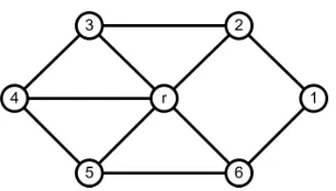
Proof. Since algorithm A4 operates on induced subgraphs of the infinite tri-angular grid graphT∞, the number of 3-cliques about vertexr is constant (cf. Figure 6).

Thus, there are a maximum of five such 3-cliques since there are six 3-cliques containing a single given vertex ofT∞ and we disregard the current 3-clique. The setP then has a maximum of 5 elements.

Finally, each elementsofP considers all elementst∈P proceedings. Since there are a maximum of 5 elements inP this requires a maximum and constant number of 4 + 3 + 2 = 4(4 + 1)/2−1 = 10 operations. Therefore, the total complexity isO(1).

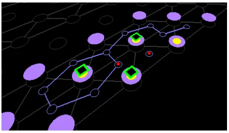
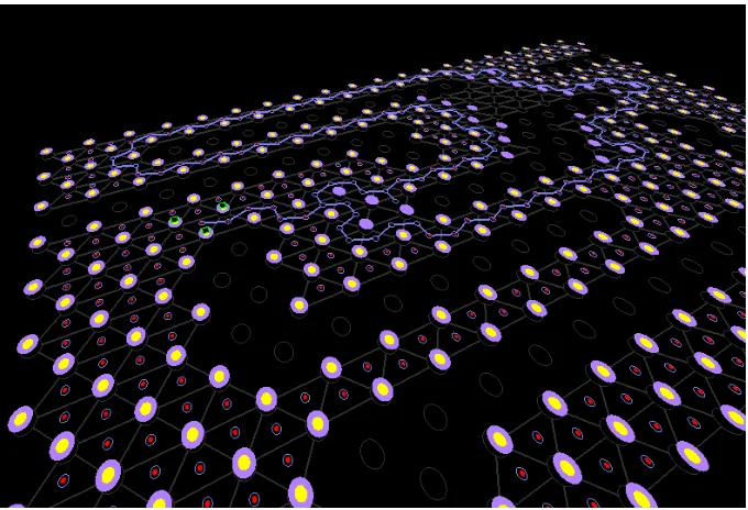
Figure 5: Dynamic graph construction

4. Analysis and Discussion

Figures 5 and 7 show example outputs of the system (algorithm A2) given different environment graphsL. The system achieves the goals set out at the beginning of this section, taking into account the restrictions imposed by the unknown environment (such as a lack of information as to thek-connectedness of the representative movement graph).

Figure 6: 3-clique formation centered onr. C={{r23},{r34},{r45},{r56}}.

4.1. Completeness

Completeness (briefly mentioned in section 2) ensures the algorithm com-pletely covers the accessible induced subgraph of an environment graphL.

Theorem 1. Let L be the localization graph of the environment, initially un-known to the 3-clique of entitiesC ={Ri} whose dual vertex is m∈M. Then the final walkΩ∗∈ Mproduced by Algorithm A2 spans the entire graphL − L0_,

whereL0 _{is the graph of unreachable vertices of the environment.}

Proof. Consider the initial known movement graphM (cf. Figure 5, for exam-ple). WhereverL(in grey) permits, each 3-clique ofLinstantiates a connected vertexm0∈M of the movement graph. Thus, the mechanism of extension exists to instantiate and connect those vertices having potential to exist, but which have not previously been disconnected. The proof is completed by induction.

By this mechanism of extension, there always exists a simple pathP ∈M of lengthl+ 1, whereP =mp1p2· · ·pl, such that there existsq∈N(pl) unvisited,

where N(pl) is the set of neighboring vertices of pl. The case for which l = 0

is simply the case for which one or more neighbors m0 of m are unvisited. If no such simple path exists then the algorithm is complete since, by definition, a path is only ever disconnected when m is a cut vertex rooting one or more biconnected components which are wholly visited or enclosed by wholly visited vertices. Thus, a simple path connecting to an unvisited biconnected component of the graph is never disconnected.

In the case the where the next move of the movement graph M relative to the 3-clique is unaltered from the previous level-1 face walk, then the next vertex within the previously calculated level-1 face (ω0 =ω+ 1) of Ω ∈M is traversed. Traversal continues until an unvisited vertex is reached, in which case the graph is dynamically extended, and the outer face walk is recalculated, thus completing the induction.

4.2. Walk Length

The system deals with unknown environment exploration with noa priori

Figure 7: Dynamic graph construction

However, in this section we present a logical argument which makes headway in understanding the walk length resulting from algorithm A2. An upper bound is given on the length of the final walk Ω∗.

To do this consideration of the key subroutines (mechanisms (i)-(v) listed in section 3.3) of the algorithm is required.

LetL∗ be the final localization graph discovered by A2, whereL∗=L − L0 and L0 _{is the graph of indiscoverable vertices. Then naturally h(Ω}∗_{) depends} on the features contained withinL∗ which, of course, directly effects the final movement graphM∗.

By mechanisms (i), (iv), and (v) the algorithm, by definition of the level-1 face algorithm, follows the boundary vertices of L∗. In addition mechanism (iii) deletes the graph vertex of all previous moves ω−1 where possible, thus reducing the graph of available future moves (before dynamic expansion).

This mechanism causes previously visited vertices to act as “walls” of the environment, thus the algorithm will not tread these vertices on its next return unless doing so would allow access to one or more unvisited regions (such as biconnected components).

We can deduce that this approach leads to a “spiders-web”, or spiraling, approach to graph discovery until all available vertices become visited.

Figure 8: Concentric level-kfaces of two regionsCandDof graphGconnected by a simple pathP =vw1w2. . . wmv0.

by visited vertices. Clearly it would be inefficient to traverse such simple paths, and the mechanism identifies and removes them using depth first search.

An inefficient property of the current mechanisms concerns the existence of biconnected components connected by a path, however short, one or more of which may contain a number of concentric level-k faces (see Figure 8). This inefficiency is highlighted by the following lemma.

Lemma 1. Let biconnected components C and D be two regions of M∗, con-nected by a simple path P =vw1w2. . . wmv0, containing quantities c and d of level-k faces respectively such thatc≥d. ThenP must be traversed 2dtimes to discoverD fully.

Proof. The previous discussion demonstrated that cut-vertices are not deleted (by mechanism (iii)) if returning to them would allow access toone or more un-visited regions. This is demonstrated in Figure 8. Traversing the outer boundary in regionC to the indicated cut-vertexv, the level-1 face, by definition, would traverse pathPto join cut-vertexv0in regionDbefore traversing its level-1 face. Traversal would proceed until v0 is rejoined and P is traversed in the reverse direction to joinv. Any remainder of the level-1 face in C would be traversed until a join side-stepped the outer face walk into the level-2 face. Note that by mechanism (iii) the level-1 face in regionD would be fully deleted (assuming no further biconnected components are connected to the level-1 face of region

D), as would that of regionC. Thus, the simple pathP is traversed exactly 2 times, with a remainingd−1 outer boundaries in regionD.

Clearly, repeating this procedure results in a total traversal of 2dtraversals of the simple pathP to fully discover regionD.

Now suppose mechanism (ii) is omitted from algorithm A2 for the moment. Then by the previous discussion a spiraling approach to discovery occurs, with recourse to theoutermost cut-vertices of the boundary of the movement graph as the boundary is traversed (bearing in mind the boundary is continuously reduced where possible by mechanism (iii)).

Therefore, the final walk length h(Ω∗) depends on the outer-boundary cut-vertices withinM. Now letDi be the ith biconnected component connected to

any other region C by a simple path P =vw1w2. . . wmv0, such that σ(C) ≥

Figure 9: The walk completes isolated regions, unlike in Figure 8

X such that each level-kface contains the vertexv0.

We may use Lemma 1 to compute the traversal cost of the simple path joining the two regions. However, before doing so, a further consideration is required:

Every time a simple path P connecting regions C to Di is traversed, the

length ofPincreases since on reachingDithe walk traverses the outer boundary

therein and returns tov0. If this was not the last level-kface of this region then the region will be revisited once more, but to reach an unvisited vertex of that region it must travel 1 vertex further than before. Therefore, each time the path is traversed, then due to mechanism (v) the path length must be noted to increase by exactly 1. Therefore, a given isolated regionDi would require

2|Pi|+ 2(|Pi|+ 2) + 2(|Pi|+ 3) +· · ·+

2(|Pi|+σ(Di))

= 2|Pi|σ(Di) + 2(2 + 3 +· · ·+σ(Di))

= 2(|Pi|σ(Di) +

σ(Di)(σ(Di) + 1)

2 −1)

= σ(Di)(2|Pi|+σ(Di) + 1)−2,

steps.

This gives the undesirable result of exiting a biconnected component multiple times, stripping the biconnected component of its level-1 face on every exit (except where additional biconnected components are attached to it)

It would be much more efficient and desirable if the system completed a biconnected component before exiting (as in Figure 9). To remedy this, the level-1 face algorithm disregards visited vertices (i.e. those corresponding to a path connecting two biconnected components) where unvisited yet known (i.e. sensed) vertices are available. This new mechanism (mechanism (vi)) is in addition to those stated in section 3.3.

Figure 10: Demonstration of Lemma 1.

effect of the next level-1 face computed to be that of the interior of the bicon-nected component. This process continues until the biconbicon-nected component is fully explored at which point the region is exited.

Given the previous discussion and the introduction of mechanism (vi), we can deduce an estimate for a maximum bound ofh(Ω∗),

h(Ω∗)≤n+ 2

p−1

X

k=1

|Pk|,

wherepis the number of biconnected components emerging asM develops and

Pk are paths connecting their centres.

5. Closing Remarks

This paper gives a solution to the difficult problem of unknown environment search using graph structures and elements of graph theory.

On imposing a virtual structure on the environment, a principle of search, basically amounting to wall following, was developed into a number of algorithms and additional mechanisms were reasoned and applied to achieve a desired result each of which improved efficiency of the search in some way.

The result is a simple, discrete, and robust ready made system of linear time complexity which is both useful in its current form yet allowing room for further development.

entities within the environment and eventual metric map construction. Previous approaches traditionally overlay the topological structure once the environment has been searched and a metric map built.

Future work is to include improvement (possibly by way of convolution) of algorithms, and theoretical improvements of the walk length upper bound. This may itself improve on the already good time complexity. Practical applications on a real world problem (such as robots) would also be a major goal.

Finally, development of algorithms to coordinatenentities for efficient search is desirable, for large team exploration, for example.

References

[1] Alboul, L. S., Abdul-Rahman, H., Haynes, P. S., Penders, J., An approach to multi-robot site exploration based on principles of self-organization,Intelligent Robotics and Applications - Third International Conference, ICIRA 2010, Shanghai, China, November 10-12, 2010. Pro-ceedings, Part II, LNCS 6425, pp. 717–729, Springer, 2010.

[2] Haynes, P. S., Alboul, L. S., 2011.Hamiltonian Walks in Embedded Planar Graphs, In preparation.

[3] Alboul, L. and Echeveria, G. and Rodrigues, M., 2004. Curvature criteria to fit curves to discrete data. EWCG 19th European Workshop on Compu-tational Geometry.

[4] Baker, B. S, 1994.Approximation algorithms for NP-complete problems on planar graphs. Journal of the Association for Computing Machinery, 41:1, pp. 153-180.

[5] Tutte, W. T., 1956.A theorem on planar graphs. Transactions of American Mathematical Society, 82, pp. 99-116.

[6] Tutte, W. T., 1977. Bridges and Hamiltonian circuits in planar graphs. Aequationes Mathematica, 15, pp. 1-33.

[7] Gerkey, B., Mataric, M., Multi-robot task allocation: Analyzing the com-plexity and optimality of key architectures. In: Proc. of the IEEE Interna-tional Conference on Robotics and Automation (ICRA) (2003).

[8] Bailey, T.; Durrant-Whyte, H., Simultaneous localization and mapping (SLAM): part II,. IEEE Robotics and Automation Magazine, V.13(3), pp. 108-117.

[10] Fox, D., Ko, J., Konolige, K., Limketkai, B., Schulz, and D., Stewart, B.: Distributed Multirobot Exploration and Mapping.Proceedings of the IEEE, Vol.94, No. 7, pp. 1325-1339, (2006).

[11] Howard, A., Mataric, M. J., Sukhatme, G. S.: Localization for mobile robot teams: A distributed MLE approach. In Experimental Robotics VIII, ser. Advanced Robotics Series, 146–166, (2002).

[12] Rekleitis, I., Dudek, G., and Milios, E. : Multi-robot collaboration for robust exploration, Annals of Mathematics and Artificial Intelligence, Vol. 31, pp. 7-40, (2001).

[13] Ludwig, L., Gini, M.: Robotic Swarm Dispersion Using Wireless Intensity Signals. In: Distributed Autonomous Robotic Systems 7, pages 135–144. Springer Japan, 2007.

[14] Mesbahi, M., Egerstedt, M.,Graph Theoretical Methods in Multiagent Net-works. Princeton University Press, 2010.

[15] Rekleitis, I., Dudek, G., and Milios, E. : Multi-robot collaboration for robust exploration, Annals of Mathematics and Artificial Intelligence, Vol. 31, pp. 7-40, (2001).

[16] Kurazume, K. R., Hirose, S.: An experimental study of a cooperative po-sitioning system. Autonomous Robots, 8(1):4352, 2000.